The ACDD Model - University of Tasmania

SCHOOL OF ECONOMICS AND FINANCEDiscussion Paper 2008-08Yet Another Autoregressive Duration Model:The ACDD ModelNagaratnam JeyasreedharanDavid E AllenJoey Wenling YangISSN 1443-8593ISBN 978-1-86295-512-7

Yet Another Autoregressive Duration Model: The ACDD ModelbyNagaratnam Jeyasreedharan, University of Tasmania*David E Allen, Edith Cowan University andJoey Wenling Yang, University of Western AustraliaAbstractThis paper contains three novelties. First, duration (intra-trade intervals) isassigned positive and negative values, based on whether it was a bid-trade orask-trade. Second, as the transformed durations are no longer “asymmetric”,a more GARCH-like alternative to the ACD model is proposed for modellingdurations. The alternative model is called the ACDD model, where the DDstands for Directional Duration. Third, using the alternative ACD formulation,persistence in durations is addressed both in the mean and the varianceequations of the ACDD model.* Corresponding author.Page 2 of 17

1 IntroductionHigh-frequency financial time series have become widely available during thepast decade or so. Records of all transactions and quoted prices are readilyavailable in pre-determined formats from many stock exchanges. An inherentfeature is that such data are irregularly spaced in time. Several approacheshave been taken to address this feature of the data.The seminal work originated with Engle and Russell (1998), where the timebetween events (trades, quotes, price changes etc.) or durations are thequantities being modeled. These authors proposed a class of models calledthe Autoregressive Conditional Duration, or ACD, models, where conditional(expected) durations are modeled in a fashion similar to the way conditionalvariances are modeled using ARCH and GARCH models of Engle (1982) andBollerslev (1986).ACD models and GARCH models share several common features, ACDmodels being commonly viewed as the counterpart of GARCH models forduration data. Both models rely on a similar economic motivation followingfrom the clustering of news and financial events in the markets. Theautoregressive ACD model allows for capturing the duration clusteringobserved in high frequency data, i.e., small (large) durations being followed byother small (large) durations in a way similar to the GARCH model accountingfor the volatility clustering. Just as a low order GARCH model is often found tosuffice for removing the dependence in squared returns, a low order ACDmodel is often successful in removing the temporal dependence in durations.Following the GARCH literature, a number of extensions to the original linearACD model by Engle and Russell (1998) have been suggested. These includethe logarithmic ACD model of Bauwens and Giot (2000), and the thresholdACD model of Zhang, Russell and Tsay (2001). The distribution associatedwith the conditional durations has also been suggested to have severaldifferent shapes. Examples include the the exponential and Weibulldistributions as in Engle and Russell (1998), and the Burr and generalizedgamma distributions suggested by Grammig and Maurer (2000) respectively.Page 3 of 17

However, a crucial assumption for obtaining QML consistent estimates of theACD model and its extensions is that the conditional expectation of durationsis correctly specified. The QML estimation yields consistent estimates and theinference procedures in this case are straightforward to implement, but thiscomes at the cost of efficiency. In practice, fully efficient ML estimates mightbe preferred.The inherent limitations in the ACD model and its extensions to date havebeen a direct consequence of the positive asymmetric density assumed for εiin all these models as time between successive trades are positive (seeHautsch (2004)). Furthermore, the assumption of iid innovations may be toostrong and inappropriate for describing the behaviour of some financialdurations. Empirical studies based on the linear ACD model often revealpersistence in durations as the estimated coefficients on lagged variables addup nearly to one. Moreover, many financial duration series show a hyperbolicdecay, i.e., significant autocorrelations up to long lags. This suggests that abetter fit might be obtained by accounting for longer term dependence indurations. Indeed, the standard ACD model imposes an exponential decaypattern on the autocorrelation function typical for stationary and invertibleARMA processes. This may be completely inappropriate in the presence oflong memory processes.In this paper we provide and slightly different approach to work originated byEngle and Russell (1998). We propose an alternative definition of durations,where positive durations depict “ask-durations” and negative durations depict“bid-durations”. This approach enables the resultant error density to besymmetrical. The resultant model is called the Autoregressive ConditionalDirectional Duration (ACDD) model.2 The basic ACDD modelThe time series of arrival times or durations between successive occurrencesof certain events associated with the trading process can be defined in anumber of ways. Examples include the time between successive trades, thePage 4 of 17

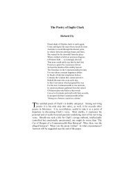
time until a price change occurs or until a pre-specified number of shares orlevel of turnover has been traded. We define directional duration as the timebetween successive trades where the trades at the ask-quotes are positiveand at the bid-quotes are negative. In doing so we are able to differentiatebetween the arrival times of bid and ask-quotes.The basic ACDD model relies on a linear parameterization of the conditionalduration, ψi, which depends on p past absolute directional durations, δ i−jand q past conditional durations, ψi − jas defined by:pψ = ω+ α δ + βψi j i−j j i−jj= 1 j=1q∑ ∑ (1.1)where δi = γi(ti − ti−1) are the directional durations and γi= 1 for an askdurationsand γi=− 1 for bid-durations with t being the trade times. Toensure positive conditional durations for all possible realizations, sufficient butnot necessary conditions are ω > 0 , α ≥ 0 , β ≥ 0 . The main assumptionbehind ACDD model is that the standardized directional durations,εδii= , (1.2)ψiare independent and identically distributed (iid) with E( ε ) = 0 andiE( ε ) = 1.Directional durations thus defined enable symmetrically distributed innovationerrors to be assumed as shown in Figure 1 below. It can be seen that thedirectional durations are both positive and negative, whereas standarddurations have positive support.2iPage 5 of 17

Standard Durations100 500Feb 1 1991Directional Durations-400 0 400Feb 1 1991Abs(Directional Durations)100 500Feb 1 1991Figure 1: Standard, Directional and |Directional| Durations in seconds (IBM data)Let f ( ε , θε) be the density function for ε with parameters θ ε. A naturalchoice convenient for estimation will be any family of suitable symmetricaldistributions. We adopt the generalized error distribution (GED) familyproposed by Nelson (1991) to capture the fat tails, if any, in the error terms. Ifa random variable ε ihas a GED with mean zero and unit variance, the PDFof εiis given by:υυ exp ⎡−( 1/ 2) εi/ λ ⎤f( εi ) =⎣⎦( υ+1 )/ υλ• 2 Γ( 1/ υ)(1.3)where1−2 / υ2⎡2 Γ( 1/ υ ) ⎤λ = ⎢Γ( 3 / υ ) ⎥⎣⎦(1.4)Page 6 of 17

and υ is a positive parameter governing the thickness of the tail behaviour ofthe distribution. When υ = 2 the above PDF reduces to the standard normalPDF; when υ < 2 , the density has thicker tails than the normal density; whenυ > 2, the density has thinner tails than the normal density. When the tailthickness parameter υ = 1, the PDF of the GED reduces to the PDF of adouble exponential distribution (analogous to the exponential distribution inthe basic ACD model of Engle and Russell (1998)).Based on the above PDF, the log-likelihood function of ACDD model withGED errors can be constructed as such maximum likelihood (ML) estimatorsfor the ACDD parameters can be obtained as opposed to the quasi-maximumlikelihood (QML) estimators used in ACD models. Furthermore, the redefinitionof durations to bid- and ask-based durations enables us to fullyadopt GARCH formulations, meaning both the mean equation and thevariance equation in the standard GARCH model and its extensions can beutilitsed.The autocorrelation properties of standard durations led to the development ofthe original ACD model where the error terms were assumed to be iid.Distributions defined on positive support typically imply a strict relationshipbetween the first moment and higher order moments and do not disentanglethe conditional mean and variance function. For example, under theexponential distribution, all higher order moments directly depend on the firstmoment. Hence the inherent restrictiveness or inflexibility encountered withACD models.In fact, a battery of tests on the IBM data (not reported in this paper) revealthat the durations, apart from being autocorrelated and having arch effects,also exhibit long range dependence (long memory) and non-stationarity. Thus,whist crucial for the ACD model and its extensions the “assumptions of iidinnovations may be too strong and inappropriate for describing the behaviourof trade durations” (see Pacurar (2006)).In the above ACDD formulation, the directional durations still exhibit longrange dependence (long memory) and non-stationarity in addition to beingPage 7 of 17

autocorrelated and arched. In addition, diurnal and day-of-the-week (DoW)components have also been observed in duration data (see …). To addressthese stylised characteristics and as several ‘trend-generating’ mechanismsmay occur simultaneously we include a SEMIFAR-type mean equation intothe ACDD model.3 The SEMIFAR-ACDD modelSemiparametric fractional autoregressive (SEMIFAR) models (see Beran andFeng (2002)) have been introduced for modelling different components in themean function of a financial time series simultaneously, such asnonparametric trends, stochastic nonstationarity, short- and long-rangedependence as well as antipersistence. SEMIFAR includes ARIMA andFARIMA processes (see Hosking (1981); Granger and Joyeux (1980)).Let d = ( − 0505 . , . ) be the fractional differencing parameter, m ∈ { 01 , } be theinteger differencing parameter, L be the lag or backshift operator, φ (L) andθ (L) be the lag polynomials in L with no common factors and all rootsoutside the unit circle and εibe white noise, then the SEMIFAR model can bedefined as (see Feng, Beran and Yu (2007)):1 dmφ(L)( −L) [( 1−L) y − g( τ ) = θ(L)ε(1.5)i i iwhere τi= t/niis the rescaled time.Similarly, in the SEMIFAR–ACDD model, the mean equation in is defined asfollows:1 dmφ(L)( −L) [( 1−L) δ − g( τ ) = θ(L)ζ(1.6)i i iwith the duration equation defined by:pψ = ω+ α ζ + βψi j i−j j i−jj= 1 j=1q∑ ∑ (1.7)Page 8 of 17

where ζiis then the adjusted directional duration. To ensure positiveconditional durations for all possible realizations, sufficient but not necessaryconditions are that ω > 0 , α ≥ 0 , β ≥ 0 . The main assumption behindSEMIFAR-ACDD model is that the standardized directional durations,εζii= , (1.8)ψiare independent and identically distributed (iid) with E( ε ) = 0 andiE( ε ) = 1.2i4 MethodologyBased on the SEMIFAR-ACDD model above and the asymptotic results forthe SEMIFAR-GARCH formulation obtained by Feng, Beran and Yu (2007),the following algorithm in S-PLUS is proposed for the practical implementationof the SEMIFAR–ACDD model:(a) Carry out data-driven SEMIFAR fitting using algorithm, AlgB in Beran andFeng (2002) to the square-root of observations to obtain g( τ ), φ (L) andθ (L);(b) Calculate the residuals ξi = δi − g( τi) and invert ξiusing φ (L) and θ (L)into ˆζi, the estimates of ζi;(c) Estimate the ACDD model using S-PLUS/GARCH software taking theresiduals of the SEMIFAR model in (b) above.The best SEMIFAR-ACDD model is then determined as follows:(a) For p = 1,pmaxand q = 1,qmaxestimate ACDD(p,q) and calculate BIC(p, q);(b) Choose the ACDD(p,q) model that minimizes the BIC. We obtain the fittedACDD model, where the BIC in S-PLUS will be used, which is given by:BIC(p, q) = -2 • log(maximized likelihood) + (log n)(p + q + 2) (1.9)Page 9 of 17

The estimated parameter vectors for the SEMIFAR and the ACDD models areasymptotically independent (see Feng, Beran and Yu (2007)). With the trendfunction in the SEMIFAR–ACDD model, it is inconvenient to select the twoequations (1.6 and 1.7) at the same time. Thus they are selected separately.The best-fit SEMIFAR model is chosen from r=0,1,2 and s=0 and the bestfitACDD model selected from p = 0,1,2 and q = 0, 1, 2 , by means of theminimal BIC.5 The DataThe dataset in this paper is the IBM data used in the seminal paper titled"Autoregressive Conditional Duration: A New Model for Irregularly SpacedTransaction Data" by Engle and Russell (1998) and downloaded fromhttp://weber.ucsd.edu/~mbacci/engle. This is to enable direct comparisons tobe made with the basic ACD model and data.A total of 60328 transactions were recorded for IBM over the 3 months oftrading on the consolidated market from November 1990 through January1991. As per the seminal paper, two days from the three months weredeleted. A halt occurred on 23 rd November and a more than one hour openingdelay occurred on 27 th December. Following Engle and Russell (1998) the firsthalf hour of the trading day (i.e. trades before 10.00am) is omitted. This is toavoid modeling the opening of the market which is characterized by a callauction followed by heavy activity. The dynamics are likely to be quite differentover this period. Furthermore, the call auction transactions are not recorded atthe same time each morning.In addition, all trades after 4.00pm were also omitted. After omitting these twodays and times, of the original 60328 transactions there were 51356observations left. Of the transactions occurring at non-unique trading times,nearly all of them corresponded with zero price movements. Engle andRussell (1998) suggest that these transactions may reflect large orders thatwere broken up into smaller pieces. As it is not clear that each piece shouldbe considered a separate transaction, the zero-second durations werePage 10 of 17

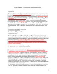
considered to be a single transaction and were deleted from the data set as inEngle and Russell (1998). After all the adjustments to the data, 46052observations were collated.In their seminal paper, Engle and Russell (1998) reported 46091 final IBMobservations. This is probably a typo (it should have been 46051) as theirother reported summary statistics for the same dataset was identical with amean duration of 28.38 seconds, maximum duration of 561 seconds andstandard deviation of 38.41 seconds. We ended up with 46052 observations,the extra 1 observation is due to the way we computed the durations.ACF0.0 0.2 0.4 0.6 0.8 1.0ar$order= 46Standard DurationACF0.0 0.2 0.4 0.6 0.8 1.0Abs(Directional Duration)ar$order= 460 10 20 30 40Lag0 10 20 30 40LagACF0.0 0.2 0.4 0.6 0.8 1.0Sqrt(Standard Duration)ar$order= 46ACF0.0 0.2 0.4 0.6 0.8 1.0Sqrt(Directional Duration)ar$order= 360 10 20 30 40Lag0 10 20 30 40LagFigure 2 ACFs of functions of Standard and Directional DurationsIt can be seen from Figure 2 that the autocorrelation properties of thestandard duration and the absolute directional durations are identical bydefinition. However, the ACF plot of the directional durations exhibit AR(MA)effects.Page 11 of 17

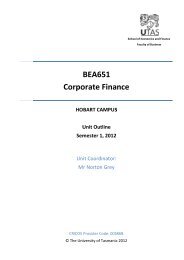
Herein the difference between standard and directional durations: first orderdependencies are fundamentally different. The inclusion of the SEMIFARequation to ACDD model ensures that the error residuals are IID. However,the second order dependencies are identical. Consequently, the conditionalduration equation remains unchanged.6 ResultsFigure 3 exhibits the adjusted durations (square-root) for both the standardand directional durations. The standard durations were adjusted using thetrend function using the SEMIFAR(0,0) model. Though this adjustment isdifferent to that done by Engle and Russell (1998) it is similar.Sqrt(Standard Durations)Directional Sqrt(Durations)2 10 18Feb 1 1991Feb 1 1991data-driven g(t)-function3.5 4.5 5.5Feb 1 1991g(t)-Adjusted Sqrt(Standard Durations)1 2 3 4 50.00 0.20-4 0 2 4data-driven g(t)-functionFeb 1 1991SEMIFAR-Adjusted Directional Sqrt(Durations)-6 -2 2 4Feb 1 1991Feb 1 1991Figure 3: Adjusted Durations (square-root)As mentioned earlier, the AlgB in Beran and Feng (2002) was used forestimating the SEMIFAR portion of the model. The trend was estimated bylocal linear regression using a kernel as the weight function. For the short-Page 12 of 17

memory effects, only an AR component was considered. The SEMIFARmodel is chosen from r = 0,1,2.lb-stat lm-stat rs-stat kpss-statAdjsqSD 10725.0039 2333.2642 1.2841 0.0444p.value 0.1AdjsqDD 30.7122 1733.0241 0.6662 0.0117p.value >0.1 0.1 >0.1Table 1: Adjusted Duration Statistics (square-root)The adjusted standard durations (ASD) are still contain autocorrelations andarch effects. The directional durations are based on the adjusted durationsand further adjusted using the SEMIFAR model. As can be seen from Table 1the ADD series have no autocorrelation and long memory, but still have archeffects. All the ADD statistics are however significantly lower than that of theASD statistics. The ACD, ACDD and SEMIFAR-ACDD models are then fittedand tested. The ACD and ACDD coefficients for the duration equations arelisted in Table 2. The duration parameters are of the same order. The GEDparameter values for all models are greater than the value of 2 for a normaldistribution."ACD" "ACDD" "SEMIFAR-ACDD""A" 0.0195 0.0174 0.018"ARCH(1)" 0.066 0.0622 0.057"GARCH(1)" 0.9191 0.9242 0.9297"dist.par" 2.9635 2.9423 2.1682Table 2: ACDD coefficients and ged-parameterThe ACD and ACDD statistics are displayed in Table 3. The ACD and ACDDmodels have dependent residuals, arch effects and non-normal distributions.The SEMIFAR-ACDD MODEL has no dependency, still has some arch effectsand non-normality in the standardized residuals.lb-stat lm-stat jb-statACD 42.1238 35.2505 10643.7801p.value 0.0002 0.0023 0ACDD 4112.4265 33.0222 780.0414p.value 0 0.0047 0SEMIFAR-ACDD 7.2107 37.4595 255.0674p.value 0.9515 0.0011 0Table 3: ACD/ACDD statisticsPage 13 of 17

The Ljung-Box statistic for the ACD model was 42.12 is of the same order ofthe reported statistic (lb-stat=38.08) in Engle and Russell (1998).The SEMIFAR-ACDD model is chosen from p = 0,1,2 and q = 0,1,2 by meansof BIC/AIC/LL. The best ACDD model fitted is the SEMIFAR-ACDD(1,2) asshown by the lowest values in Table 4.acdd01 acdd02 acdd10 acdd11 acdd12 acdd20 acdd21 acdd22AIC 141633 143134 140967 139181 139173 140722 139169 140768BIC 141659 143169 140993 139216 139217 140757 139213 140820LL -70814 -71563 -70481 -69587 -69582 -70357 -69580 -70378Table 4: BIC, AIC and LL-values for ACDD modelsConditional Durations20 40 60 80 100 120 140 160Feb 1 1991Figure 4: ACD and SEMIFAR-ACDD conditional durationsIn Figure 4 above, the points in black depict the conditional durations from theSEMIFAR-ACDD model, whereas the grey lines depict the conditionaldurations from the ACD model. The results are similar but not identical.Page 14 of 17

7 ConclusionThis paper modifies the ACD approach to a SEMIFAR–ACDD model so thattrends and long memory in durations can be modelled using a moreparsimonious parameterisation. A semi-parametric estimation procedure isproposed for the trend function. Asymptotic results on the SEMIFAR-GARCHmodel as reported by Feng, Beran and Yu (2007) are extended to theSEMIFAR-ACDD model.The important property that the estimates of the FARIMA and ACDDparameter vectors are independent of each other, allow us to apply the datadrivenSEMIFAR algorithms to estimate the trend and the FARIMAparameters in the SEMIFAR–ACDD model. The ACDD parameters from theapproximated ACDD innovations are calculated by inverting the finalresiduals.The results show that the proposed algorithm and model can be used tomodel dependencies in durations data. Further possible extensions to themodel include leverage effects and the range of GARCH-type extensions.ReferencesBauwens, L, and P Giot, 2000, The Logarithmic ACD Model: an Application tothe Bid-Ask Quote Process of Three NYSE Stocks, Annalesd’Économie et de Statistique 60, 117-149.Beran, J, and Y Feng, 2002, Iterative plug-in algorithms for SEMIFARmodels—definition, convergence and asymptotic properties, Journal ofComputational Graphical Statistics 11, 690-713.Beran, J, and Y Feng, 2002, SEMIFAR models—a semiparametric frameworkfor modelling trends, long-range dependence and nonstationarity,Computational Statistics and Data Analysis 40, 393-419.Bollerslev, T, 1986, Generalized autoregressive conditionalheteroskedasticity, Journal of Econometrics 31, 307-327.Engle, R F, 1982, Autoregressive Conditional Heteroscedasticity withEstimates of the Variance of United Kingdom Inflation, Econometrica50, 987-1007.Page 15 of 17

Engle, R F, and J R Russell, 1998, Autoregressive conditional duration: A newmodel for irregularly spaced transaction data, Econometrica 66, 1127-1162.Feng, Y, J Beran, and K Yu, 2007, Modelling financial time series withSEMIFAR-GARCH model. , 18, 395-412., IAM Journal of ManagmentMathematics 18, 395-412.Grammig, J, and K O Maurer, 2000, Non-Monotonic Hazard Functions andthe Autoregressive Conditional Duration Model, Econometrics Journal3, 16-38.Granger, C W J, and R Joyeux, 1980, An introduction to long-memory timeseries models and fractional differencing, Journal of Time SeriesAnalysis 1, 15-30.Hautsch, N, 2004. Modelling irregularly spaced financial data : theory andpractice of dynamic duration models (Springer, London).Hosking, J R M, 1981, Fractional differencing, Biometrika 68, 165-176.Zhang, M Y, J R Russell, and R S Tsay, 2001, A nonlinear autoregressiveconditional duration model with applications to financial transactiondata, Journal of Econometrics 104, 179.Page 16 of 17

School of Economics and Finance Discussion Papers2008-01 Calorie Intake in Female-Headed and Male Headed Households in Vietnam, Elkana Ngwenya2008-02 Determinants of Calorie Intake in Widowhood in Vietnam, Elkana Ngwenya2008-03 Quality Versus Quantity in Vertically Differentiated Products Under Non-Linear Pricing, HughSibly2008-04 A Taxonomy of Monopolistic Pricing, Ann Marsden and Hugh Sibly2008-05 Vertical Product Differentiation with Linear Pricing, Hugh Sibly2008-06 Teaching Aggregate Demand and Supply Models, Graeme Wells2008-07 Demographic Demand Systems with Application to Equivalence Scales Estimation andInequality Analysis: The Australian Evidence", Paul Blacklow, Aaron Nicholas and Ranjan Ray2008-08 Yet Another Autoregressive Duration Model: The ACDD Model, Nagaratnam Jeyasreedharan,David E Allen and Joey Wenling Yang2008-09 Substitution Between Public and Private Consumption in Australian States, Anna Brown andGraeme Wells2007-01 Dietary Changes, Calorie Intake and Undernourishment: A Comparative Study of India andVietnam, Ranjan Ray2007-02 A Re-examination of the Real Interest Parity Condition Using Threshold Cointegration, ArushaCooray2007-03 Teaching Aggregate Demand and Supply Models, Graeme Wells2007-04 Markets, Institutions and Sustainability, Ella Reeks2007-05 Bringing Competition to Urban Water Supply, Hugh Sibly and Richard Tooth2007-06 Changes in Indonesian Food Consumption Patterns and their Nutritional Implications, ElkanaNgwenya and Ranjan Ray2007-07 The Term Spread and GDP Growth in Australia, Jacob Poke and Graeme Wells2007-08 Moving Towards the USDA Food Guide Pyramid Food: Evidence from Household Food GroupChoice in Vietnam, Elkana Ngwenya2007-09 The Determinants of the Quantity-Quality Balance in Monopoly, Hugh Sibly2007-10 Rationing Recreational Access to Wilderness and Other Natural Areas, Hugh Sibly2007-11 Yet Another Trading Simulation: The Nonimmediacy Model, Nagaratnam JeyasreedharanCopies of the above mentioned papers and a list of previous years’ papers are available onrequest from the Discussion Paper Coordinator, School of Economics and Finance, Universityof Tasmania, Private Bag 85, Hobart, Tasmania 7001, Australia. Alternatively they can bedownloaded from our home site at http://www.utas.edu.au/ecofin ||Page 17 of 17