Optimal Power Control for Multi-Hop Software Defined Radio Networks

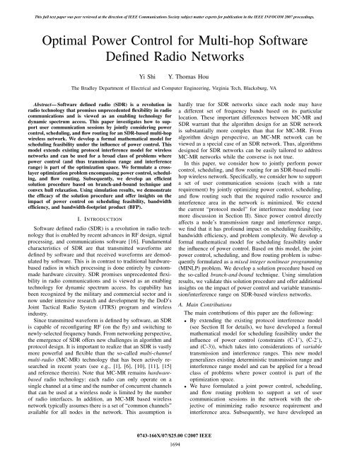
This full text paper was peer reviewed at the direction of IEEE Communications Society subject matter experts for publication in the IEEE INFOCOM 2007 proceedings.Optimal Power Control for Multi-hop SoftwareDefined Radio NetworksYi ShiY. Thomas HouThe Bradley Department of Electrical and Computer Engineering, Virginia Tech, Blacksburg, VAAbstract— Software defined radio (SDR) is a revolution inradio technology that promises unprecedented flexibility in radiocommunications and is viewed as an enabling technology fordynamic spectrum access. This paper investigates how to supportuser communication sessions by jointly considering powercontrol, scheduling, and flow routing for an SDR-based multi-hopwireless network. We develop a formal mathematical model forscheduling feasibility under the influence of power control. Thismodel extends existing protocol interference model for wirelessnetworks and can be used for a broad class of problems wherepower control (and thus transmission range and interferencerange) is part of the optimization space. We formulate a crosslayeroptimization problem encompassing power control, scheduling,and flow routing. Subsequently, we develop an efficientsolution procedure based on branch-and-bound technique andconvex hull relaxation. Using simulation results, we demonstratethe efficacy of the solution procedure and offer insights on theimpact of power control on scheduling feasibility, bandwidthefficiency, and bandwidth-footprint product (BFP).I. INTRODUCTIONSoftware defined radio (SDR) is a revolution in radio technologythat is enabled by recent advances in RF design, signalprocessing, and communications software [16]. Fundamentalcharacteristics of SDR are that transmitted waveforms aredefined by software and that received waveforms are demodulatedby software. This is in contrast to traditional hardwarebasedradios in which processing is done entirely by custommadehardware circuitry. SDR promises unprecedented flexibilityin radio communications and is viewed as an enablingtechnology for dynamic spectrum access. Its capability hasbeen recognized by the military and commercial sector and isnow under intensive research and development by the DoD’sJoint Tactical Radio System (JTRS) program and wirelessindustry.Since transmitted waveform is defined by software, an SDRis capable of reconfiguring RF (on the fly) and switching tonewly-selected frequency bands. From networking perspective,the emergence of SDR offers new challenges in algorithm andprotocol design. It is important to realize that an SDR is vastlymore powerful and flexible than the so-called multi-channelmulti-radio (MC-MR) technology that has been actively researchedin recent years (see e.g., [1], [6], [10], [11], [15]and reference therein). Note that MC-MR remains hardwarebasedradio technology: each radio can only operate on asingle channel at a time and the number of concurrent channelsthat can be used at a wireless node is limited by the numberof radio interfaces. In addition, an MC-MR based wirelessnetwork typically assumes there is a set of “common channels”available for all nodes in the network. This assumption ishardly true for SDR networks since each node may havea different set of frequency bands based on its particularlocation. These important differences between MC-MR andSDR warrant that the algorithm design for an SDR networkis substantially more complex than that for MC-MR. Fromalgorithm design perspective, an MC-MR network can beviewed as a special case of an SDR network. Thus, algorithmsdesigned for SDR networks can be easily tailored to addressMC-MR networks while the converse is not true.In this paper, we consider how to jointly perform powercontrol, scheduling, and flow routing for an SDR-based multihopwireless network. Specifically, we consider how to supporta set of user communication sessions (each with a raterequirement) by jointly optimizing power control, scheduling,and flow routing such that the required radio resource andinterference area in the network is minimized. We extendthe current “protocol model” for interference modeling (seemore discussion in Section II). Since power control directlyaffects a node’s transmission range and interference range,we find that it has profound impact on scheduling feasibility,bandwidth efficiency, and problem complexity. We develop aformal mathematical model for scheduling feasibility underthe influence of power control. Based on this model, the jointpower control, scheduling, and flow routing problem is subsequentlyformulated as a mixed integer nonlinear programming(MINLP) problem. We develop a solution procedure based onthe so-called branch-and-bound technique. Using simulationresults, we validate this solution procedure and offer additionalinsights on the impact of power control and variable transmission/interferencerange on SDR-based wireless networks.A. Main ContributionsThe main contributions of this paper are the following:• By extending the existing protocol interference model(see Section II for details), we have developed a formalmathematical model for scheduling feasibility under theinfluence of power control (constraints (C-1’), (C-2’),and (C-3)), which takes into considerations of variabletransmission and interference ranges. This new modelgeneralizes existing deterministic transmission range andinterference range model and can be applied for a broadclass of problems where power control is part of theoptimization space.• We have formulated a joint power control, scheduling,and flow routing problem to support a set of usercommunication sessions in the network with the objectiveof minimizing radio resource requirement andinterference area. Subsequently, we have developed an0743-166X/07/$25.00 ©2007 IEEE1694

This full text paper was peer reviewed at the direction of IEEE Communications Society subject matter experts for publication in the IEEE INFOCOM 2007 proceedings.efficient solution procedure based on branch-and-boundtechnique and convex hull relaxation to solve this crosslayeroptimization problem. The solution obtained via ourapproach yields a (1 − ε) optimal solution, where ε is asmall error tolerance reflecting our desired accuracy inthe final solution.• By applying the solution procedure on sample randomnetworks, we have demonstrated quantitatively that powercontrol has significant impact on scheduling feasibility,bandwidth efficiency, and bandwidth-footprint product(BFP). This confirms the critical need of incorporatingpower control under the protocol interference model forfuture wireless network research.43651 2(a) No power control.43651 2(b) With power control.II. RELATED WORKRelated work on MC-MR and its relationship with SDRnetworks are discussed in Section I. In the rest of this section,we focus our review on cross-layer wireless network researchinvolving interference modeling.Currently, there are two popular interference models,namely, the physical model and the protocol model. Under thephysical model (e.g., [2], [4], [5], [7], [8], [11]), a transmissionis considered successful if and only if the signal to interferenceand noise ratio (SINR) exceeds a certain threshold, wherethe interference includes all other concurrent transmissions.Since the calculation of a link’s capacity involves not onlythe transmission power on this link, but also the transmissionpower on interference links, it is quite difficult to obtainan optimal solution whenever link capacity is involved. In[2], Behzad and Rubin found that for the special case wheneach node uses the same transmission power, then maximumtransmission power should be used. However, for the generalcase where each node can adjust its transmission powerindependently, optimal solution is not available. Layered (decoupled)solution approaches were proposed in [4], [5], [7],which yield sub-optimal solutions. In [8], [11], although thelower and upper bounds for transport capacity are obtained(asymptotically), the exact optimal value remains unknown.Under the so-called protocol model [8], a transmission isconsidered successful if and only if the receiving node is in thetransmission range of the corresponding transmitting node andis out of the interference range of all other transmitting nodes.Under the protocol model, related work can be classified intotwo categories. In the first category, e.g., [8], [11] (under theso-called “random networks”) and [1], [9], [10], [12], [14],[19], the transmission power is fixed. This corresponds to thespecial case of Q = 1 to be discussed later in this paper.Since both the transmission range and interference range arefixed here, the interference relationship among the links areeasy to identify. In the second category, i.e., [8], [11] (underthe so-called “arbitrary networks”) and [3], power control isconsidered but only for wireless networks with certain specialassumptions that may not reflect wireless networks consideredin practice. For example, although power control is consideredin [3], there is an assumption of no inter-link interference (alsocalled secondary interference [3]) within the network. In [8],[11], power control is considered for the so-called “arbitrarynetworks,” within which the location for each node and itsFig. 1.A 3-link network.traffic pattern can be arbitrarily changed to optimize transportcapacity. Although results for arbitrary networks do yield sometheoretical insights, they are far from reflecting what happensfor wireless networks in practice, which are mostly randomnetworks [8].In this paper, we consider the case of power control underthe protocol model for general wireless networks (without anyspecial assumptions), i.e., random networks [8]. Such approachcaptures the most general characteristics of wireless networkencountered in practice.III. IMPACT OF POWER CONTROLIn this section, we examine the impact of power controlon scheduling feasibility, bandwidth efficiency, and problemcomplexity in a multi-hop SDR network. But first, we needto have a clear understanding on the notion of transmissionand interference ranges in a wireless network as well as thenecessary and sufficient condition for successful transmission.A. Transmission and Interference RangesWe follow the protocol model as discussed in Section II. Ina wireless network, each node is associated with a transmissionrange and an interference range. Both transmission andinterference ranges directly depend on a node’s transmissionpower and propagation gain. For transmission from node i tonode j, a widely-used model for propagation gain g ij isg ij = d −nij , (1)where d ij is the physical distance between nodes i and jand n is the path loss index. 1 In this context, we assume adata transmission from node i to node j is successful onlyif the received power at node j exceeds a power threshold,say α. Suppose node i’s transmission power is p and denotethe transmission range of this node as R T (p). Then based ong ij · p ≥ α and (1), the transmission range of this node is( p) 1/nR T (p) = . (2)αSimilarly, we assume that an interference power is nonnegligibleonly if it exceeds a threshold, say β at a receiver.1 In this paper, we consider a uniform gain model. The case of non-uniformgain model can be extended without much technical difficulty.1695

This full text paper was peer reviewed at the direction of IEEE Communications Society subject matter experts for publication in the IEEE INFOCOM 2007 proceedings.Denote the interference range of a node as R I (p). Thenfollowing the same taken as the derivation for the transmissionrange, the interference range of a node is( ) 1/n pR I (p) = .βNote that the interference range is greater than the transmissionrange at a node, i.e., R I (p) >R T (p) since β < α.Asanexample, in Fig. 1(a), we have three unicast communicationlinks 1 → 2, 3 → 4, and 5 → 6. For each transmitting node(1, 3, and 5), there are two circles centered around it, with theinner circle (dashed) representing transmission range and theouter circle (solid) representing interference range.B. Necessary and Sufficient Condition for Successful TransmissionScheduling for transmission at each node in the network canbe done either in time domain or frequency domain. In thispaper, we consider scheduling in the frequency domain in theform of frequency bands. In an SDR network, each node hasa set of frequency bands that it may use for transmission andreceiving. Suppose that band m is available at both node i andnode j and denote p m ij the transmission power from node i tonode j in frequency band m. Then to schedule a successfultransmission from node i to node j, the following necessaryand sufficient condition, expressed as two constraints, must bemet. The first constraint (C-1) is that receiving node j mustbe physically within the transmission range of node i, i.e.,( pm ) 1/n(C-1) d ij ≤ R T (p m ijij )=.αThe second constraint (C-2) is that the receiving node j mustnot fall in the interference range of any other node k (k ∈N,k ≠ i) that is transmitting in the same band, i.e.,(C-2) d jk ≥ R I (p m kh) =( pmkhβ) 1/n.where h is the receiving node of node k.As an example, Fig. 1(a) shows a network with three links(1 → 2, 3 → 4, and 5 → 6). The transmission and interferenceranges for each transmitting node (1, 3, and 5)areshowninthefigure. Clearly, each receiving node falls in the transmissionrange of its respective transmitting node. Further, we can seethat both receiving nodes 2 and 6 fall in the interference rangeof node 3. Thus, when link 3 → 4 is using a frequency bandm for transmission, link 1 → 2 and link 5 → 6 should not usethe same band. It should also be noted that when link 3 → 4is not using a frequency band m, both link 1 → 2 and link5 → 6 may use band m. This is because that receiving node2 does not fall in node 5’s interference range and receivingnode 6 does not fall in node 1’s interference range.C. Impact of Power ControlIn this paper, we investigate the case that each node in anSDR network has power control capability. That is, in additionto being able to transmit at full power P , a node can alsotransmit at any intermediate power between 0 and P . As onemight expect, such freedom on power control has significantimpact on design space. In the rest of this section, weillustrate the impact of power control on scheduling feasibility,bandwidth efficiency, and problem complexity.Scheduling Feasibility. Constraint (C-2) says that a receivingnode j (corresponding to transmitting node i on bandm) must not fall in the interference range of any other nodek that is transmitting in the same band. In the absence ofpower control, the interference ranges for all the nodes in thenetwork are fixed and there is hardly much we can do once weencounter an infeasibility scenario in scheduling. On the otherhand, when power control capability is available, we couldadjust the transmission power and thus reduce the interferencerange of some node so as to achieve scheduling feasibility.We use an example to illustrate this important point. Recallthat in Fig. 1(a), where there is no power control (and thus thetransmission ranges and interference ranges for transmittingnodes 1, 3, and 5 are deterministic and shown in the figure),once link 3 → 4 is active (i.e., in transmission) in a frequencyband m, then neither link 1 → 2 nor link 5 → 6 shall be activein the same frequency band. If frequency band m is the onlyband available for these links, then it is impossible to scheduletransmissions on links 1 → 2 and 5 → 6. Now consider thateach node has the power control capability and can adjusttransmission power anywhere in [0, P]. In this setting, node3 could reduce its transmission power while still maintainingdata transmission to node 4 (see Fig. 1(b)). Now receivingnodes 2 and 6 are no longer in node 3’s interference range.As a result of this, both transmitting nodes 1 and 5 can transmitin the same frequency band m simultaneously. In other words,power control could enable scheduling feasibility.Bandwidth Efficiency. Power control capability has theadditional benefit of reducing spectrum bandwidth requirementin the network. This is a direct consequence of the schedulingfeasibility benefit discussed above.Continuing the previous example, in Fig. 1(a), when thereis no power control, one frequency band is inadequate tosupport all three links and we need at least two frequencybands in the network. However, when there is power control,in Fig. 1(b), we only need one frequency band to supportall three links. In general, one should expect once powercontrol is employed, the spectrum bandwidth requirement canbe reduced significantly for meeting the same communicationobjective than the case when there is no power control.Problem Complexity. When power control is allowed, thetransmission and interference ranges of a node can be adjustedsince both of them are functions of this node’s transmissionpower. It is not hard to realize that the design space foralgorithm or optimization solution procedure becomes substantiallylarger than the case when there is no power control.As a result, mathematical modeling, problem formulation,and solution procedure are also expected to be much morecomplex and interesting. In the rest of this paper, we explorethis problem in the context of multi-hop SDR-based ad hocnetworks.1696

This full text paper was peer reviewed at the direction of IEEE Communications Society subject matter experts for publication in the IEEE INFOCOM 2007 proceedings.IV. MATHEMATICAL MODELINGWe consider an ad hoc network consisting of a set of Nnodes. Unlike MC-MR networks where the set of availablefrequency bands at each node is identical, in an SDR network,the set of available frequency bands at each node depends onits location and may not be the same. For example, at node i,its available frequency bands may consist of bands I, III, and Vwhile at a different node j, its available frequency bands mayconsist of bands I, IV, and VI, and so forth. More formally,denote M i the set of available frequency bands at node i. Forsimplicity, we assume the bandwidth of each frequency bandis W . 2 Denote M the set of all frequency bands present inthe network, i.e., M = ⋃ i∈N M i.A. Scheduling and Power ControlIn Section III, we discussed the necessary and sufficientcondition for successful transmission and impact of powercontrol on scheduling feasibility. In this section, we formalizethese ideas into a mathematical model in the general contextof multi-hop SDR networks.Suppose that band m is available at⋂both node i and nodej, i.e., m ∈M ij , where M ij = M i Mj . Denote{x m 1 If node i transmits data to node j on band m,ij =0 otherwise.As mentioned earlier, we consider scheduling in the frequencydomain and thus once a band m ∈M i is used by node i fortransmission to node j, this band cannot be used again bynode i to transmit to a different node. That is,∑(C-3)x m ij ≤ 1 ,j∈T miwhere Tim is the set of nodes that are within the transmissionrange from node i under full power P on band m.Denote RTmax the maximum transmission range of a nodewhen it transmits at full power P . Then based on (2), we haveRTmax = R T (P )= ( )P 1/n.α Thus, we have α =P(RT max ). nThen for a node transmitting at a power p ∈ [0, P], itstransmission range isR T (p)=( [ p 1/n p(Rmax=Tα)P) n] 1/n ( p) 1/n= RmaxT . (3)PSimilarly, denote RImax the maximum interference range ofa node when it transmits at full power P . Then for a nodetransmitting at a power p ∈ [0, P], its interference range is( p) 1/nR I (p) = RmaxI . (4)PRecall that Tim denotes the set of nodes that are within thetransmission range from node i under full power P on band m,we have Tim = {j : d ij ≤ RTmax ,j ≠ i, m ∈M j }. Similarly,denote Ijm the set of nodes that can make interference onnode j on band m under full power P , i.e., Ijm = {k : d jk ≤, T m ≠ ∅}.R maxIk2 The case of heterogeneous bandwidth for each frequency band can beeasily extended.Note that the definitions of Ti m and Ij m are both based onfull transmission power P . When power level p is below P ,the corresponding transmission and interference ranges willbe smaller. As a result, it is necessary to keep track of the setof nodes fall in the transmission range and the set of nodesthat can produce interference whenever transmission powerchanges at a node.Recall the two constraints (C-1) and (C-2) for successfultransmission from node i to node j in (3) and (4), respectively,we haved ij ≤R T (p m ij )=( pmijP) pd jk ≥R I (pkh)=( m m 1/nkhRImaxP) 1/nR maxT (5)(k ∈I m j,k≠i, h∈Tmk ).(6)Based on (5) and (6), we have the following requirements forthe transmission link i → j and interfering link k → h:{ [( )dijnP, ]p m ∈R PijTmax If x m ij =1,=0 If x m ij =0.{ ( )dkjnp m kh ≤ R P If xmImaxij =1,(k ∈IP If x m j m ,k≠i, h∈Tk m ) .ij =0.Mathematically, these requirements can be re-written as[( ) n ](C-1’) p m dijij ∈Px m ij ,Px m ij(C-2’) p m kh ≤P −RTmax[1−(dkjR maxI) n ]Px m ij (k ∈I m j ,k≠i, h∈T mk ) .Recall that we consider scheduling in the frequency domainand in (C-3), we state that once a band m is used by nodei for transmission to node j, this band cannot be used againby node i to transmit to a different node. In addition, forsuccessful scheduling in frequency domain, the following twoconstraints must also hold:(C-4) For a band m ∈ M j that is available at node j,this band cannot be used for both transmission andreceiving. That is, if band m is used at node j fortransmission (or receiving), then it cannot be usedfor receiving (or transmission).(C-5) Similar to constraint (C-3) on transmission, node jcannot use the same band m ∈M j for receivingfrom two different nodes.It turns out that the above two constraints are embedded in(C-1’) and (C-2’). That is, once (C-1’) and (C-2’) are satisfied,then both constraints (C-4) and (C-5) are also satisfied. Thisresult is formally stated in the following lemma.Lemma 1: If transmission powers on every transmissionlink and interference link satisfy (C-1’) and (C-2’) in thenetwork, then (C-4) and (C-5) are also satisfied.Proof. Note that (C-4) can be viewed as “self-interference”avoidance constraint where at the same node j, its transmissionto another node h on band m interferes its reception from nodei in the same band.• To show that (C-1’) and (C-2’) lead to (C-4), we firstlet k = j in (C-2’). Then (C-2’) degenerates into p m jh ≤1697

This full text paper was peer reviewed at the direction of IEEE Communications Society subject matter experts for publication in the IEEE INFOCOM 2007 proceedings.P −Px m ij since d jj =0. If node j is receiving from nodei on band m, i.e., x m ij =1, then pm jh ≤ P − Pxm ij( ) =0.nSince p m jh ≥ djhR PxmTmax jhin (C-1’), we have that x m jhmust be 0. That is, if node j is receiving from node i onband m, then node j cannot transmit to a node h in thesame band.• Now suppose node j is transmitting to node h on bandm, i.e., x m jh= 1. We will show that this will lead tox m ij =0. This can be proved by contradiction. That is, ifx m ij =1, then we have just proved in the above paragraphthat x m jh=0. But this contradicts our initial assumptionthat x m jh =1. Therefore, xm ij must be 0. That is, if node jis transmitting to node h on band m, then node j cannotuse the same band for receiving from a node i.Combining the above two results, we have that (C-4) holds.We now prove that (C-1’) and (C-2’) also leads to (C-5).Again the proof is based on contradiction. Suppose that (C-5)does not hold. Then node j can receive from two differentnodes i and k on the same band m, i.e., x m ij =1and xm kj =1.Note that link k → j can be viewed as an interfering linkto link i → j. This corresponds to letting h =(j in (C-2’).) nThen from (C-2’), since x m ij =1,wehavepm kj ≤ dkjP .RImax( ) nOn the other hand, by (C-1’), we have p m kj≥ dkjR P .TmaxHowever, the above two inequalities cannot hold simultaneously(contradiction) since we have RImax >RTmax . Thus, theinitial assumption that (C-5) does not hold is incorrect and theproof is complete.□The significance of Lemma 1 is that since (C-4) and (C-5)are embedded in (C-1’) and (C-2’), it is sufficient to considerconstraints (C-1’), (C-2’), and (C-3) for scheduling and powercontrol.B. Flow RoutingWe consider an ad hoc network consisting a set of Nnodes. Among these nodes, there is a set of L active usercommunication (unicast) sessions. Denote s(l) and d(l) thesource and destination nodes of session l ∈Land r(l) the raterequirement (in b/s) of session l. To route these flows fromits respective source node to destination node, it is necessaryto employ multi-hop due to limited transmission range of anode. Further, to have better load balancing and flexibility, itis desirable to employ multi-path (i.e., allow flow splitting).This is because a single path is overly restrictive and may notyield optimal solution.Mathematically, this can be modeled as follows. Denotef ij (l) the data rate on link (i, j) that is attributed to sessionl, where i ∈N,j ∈T i = ⋃ m∈M iTim , and l ∈L. If node iis the source node of session l, i.e., i = s(l), then∑j∈T if ij (l) =r(l) . (7)If node i is an intermediate relay node for session l, i.e., i ≠s(l) and i ≠ d(l), thenj≠s(l)∑j∈T if ij (l) =k≠d(l)∑k∈T if ki (l) . (8)If node i is the destination node of session l, i.e., i = d(l),then∑k∈T if ki (l) =r(l) . (9)It can be easily verified that once (7) and (8) are satisfied, (9)must also be satisfied. As a result, it is sufficient to have (7)and (8) in the formulation.In addition to the above flow balance equations at each nodei ∈N for session l ∈L, the aggregated flow rates on eachlink cannot exceed this link’s capacity. Under p m ij ,wehave∑s(l)̸=j,d(l)̸=il∈Lf ∑ij(l)≤ c m ij =∑ (W log 2m∈M ij m∈M ij1+ gijηW pm ij), (10)where η is the ambient Gaussian noise density. Note thatthe denominator inside the log function contains only ηW.This is due to the use of protocol interference modeling, i.e.,when node i is transmitting to node j on band m, then theinterference range of all other nodes in this band should notcontain node j. Thus, protocol modeling significantly helps tosimplify the calculation of link capacity c m ij .V. PROBLEM FORMULATIONObjective Function. In the last section, we presenteda mathematical model for constraints on scheduling, powercontrol, and flow routing. Under these constraints, a number ofobjective functions can be considered for problem formulation.A commonly used objective is to maximize network capacity,which can be expressed as maximizing a scaling factor forall the rate requirements of the communication sessions inthe network (see, e.g. [1], [10]). In this paper, we consideranother objective called “bandwidth-footprint-product” (BFP),which better characterizes the spectrum and space occupancyfor an SDR network. The BFP was first introduced by Liu andWang in [12]. The so-called “footprint” refers the interferencearea of a node under a given transmission power, i.e., π ·(R I (p)) 2 . Since each node in the network will use a numberof bands for transmission and each band will have a certainfootprint corresponding to its transmission power, an importantobjective is to minimize network-wide BFP, which is the sumof BFPs among all the nodes in the network. That is, ourobjective is to minimize∑ ∑ ∑W · π(R I (p m ij )) 2 ,i∈N m∈M ij∈T miwhich is equal to π(RImax ) 2∑ ∑i∈N∑m∈M ij∈T miW( pm)ij 2/n.PNote that although we consider equal bandwidth for eachfrequency band in the network, the case where each frequencyband is of different bandwidth can also be formulated andsolved via the solution procedure outlined in the next section.1698

This full text paper was peer reviewed at the direction of IEEE Communications Society subject matter experts for publication in the IEEE INFOCOM 2007 proceedings.Discretization of Transmission Powers. For power control,we allow the transmission power to be adjusted between 0 andP . In practice, the transmission power can only be tuned intoa finite number of discrete levels between 0 and P . To modelthis discrete version of power control, we introduce an integerparameter Q that represents the total number of power levelsto which a transmitter can be adjusted, i.e., 0, 1 Q P, 2 QP, ···,P.Denote qij m ∈{0, 1, 2, ···,Q} the integer power level for pm ij ,i.e., p m ij = qm ijQP . Then (C-1’), (C-2’), and (10) can be rewrittenas follows:[( )qij m dij n ]∈R QxmTmax ij ,Qx m ij , (11)[ ( )qkh m dkj n ]≤Q− 1−RImax Qx m ij (k ∈Ij m ,k≠i, h∈Tk m ) , (12)∑ s(l)̸=j,d(l)̸=il∈Lf ij(l) ≤ ∑ ()m∈M ijW log 2 1+ g ij PηWQ qm ij .Problem Formulation. Putting together the objective functionand all the constraints for scheduling, power control, andflow routing, we have formulated an optimization problem inthe form of mixed-integer non-linear programming (MINLP),which is NP-hard in general. In the next section, we developa solution procedure based on the branch-and-bound approach[13] and convex hull relaxation.A. OverviewVI. A SOLUTION PROCEDUREWe find that the so-called branch-and-bound approach [13]is most effective in solving our optimization problem. Underthis approach, we aim to provide a (1 − ε) optimal solution,where ε is a small positive constant reflecting our desiredaccuracy in the final solution. Initially, branch-and-boundanalyzes partition variables, i.e., all discrete variables andall variables in a non-linear term. For our problem, thesevariables include all x m ij ’s and qm ij ’s. Then branch-and-bounddetermines the value set for each partition variable. That is,we have x m ij ∈{0, 1} and qm ij ∈{0, 1, 2, ···,Q}. Byusingsome relaxation technique, branch-and-bound obtains a linearrelaxation for the original MINLP problem and its solutionprovides a lower bound (LB) to the objective function. Aswe shall show shortly, this critical step is made possible bythe convex hull relaxation for non-linear discrete terms. Withthe relaxation solution as a starting point, branch-and-bounduses a local search algorithm to find a feasible solution to theoriginal problem, which provides an upper bound (UB)fortheobjective function. If the obtained lower and upper bounds areclose to each other, i.e., LB ≥ (1 − ε)UB, we are done.If the relaxation errors for non-linear terms are not small,then the upper bound UB could be far away from the lowerbound LB. To close this gap, we must have a tighter linearrelaxation, i.e., with smaller relaxation errors. This could beachieved by further narrowing down the value sets of partitionvariables. Specifically, branch-and-bound selects a partitionvariable with the maximum relaxation error and divides itsvalue set into two sets by its value in the relaxation solution.Then the original problem (denoted as problem 1) is dividedinto two new problems (denoted as problem 2 and problem 3).(q ) 2/nKmu ij(q ) 2/n 0q 0Fig. 2.(q 1) 2/n (q 2) 2/n (q K−1) 2/nq 1q mq 2 q K−1ijIllustration of convex hull for a discrete term.Again, branch-and-bound performs relaxation and local searchon these two new problems. Now we have lower bounds LB 2and LB 3 for problems 2 and 3, respectively. We also havefeasible solutions that provide upper bounds UB 2 and UB 3for problems 2 and 3, respectively. Since the relaxations inproblems 2 and 3 are both tighter than that in problem 1,we have UB 2 ,UB 3 ≤ UB 1 and LB 2 ,LB 3 ≥ LB 1 .Foraminimization problem, the lower bound of the original problemis updated from LB = LB 1 to LB = min{LB 2 ,LB 3 }.Also, the best feasible solution to the original problem isthe solution with a smaller UB i . Then the upper boundof the original problem is updated from UB = UB 1 toUB = min{UB 2 ,UB 3 }. As a result, we now have smallergap between UB and LB. IfLB ≥ (1 − ε)UB, we are done.Otherwise, we choose a problem with the minimum lowerbound and perform partition for this problem.Note that during the iteration process for branch-and-bound,if we find a problem z with LB z ≥ (1 − ε)UB, thenwe can conclude that this problem cannot provide muchimprovement on UB. That is, further branch on this problemwill not yield much improvement and we can thus remove thisproblem from further consideration. Eventually, once we findLB ≥ (1 − ε)UB or the problem list is empty, branch-andboundprocedure terminates. It has been shown that under verygeneral conditions, a branch-and-bound solution procedurealways converges [17]. Moreover, although the worst-casecomplexity of such a procedure is exponential, the actualrunning time could be acceptable if all partition variables areinteger variables (e.g., the problem considered in this paper).In the rest of this section, we develop important componentsin the branch-and-bound solution procedure.B. Linear RelaxationDuring each iteration of the branch-and-bound procedure,we need a relaxation technique to obtain a lower bound ofthe objective function. For a non-linear discrete term, thiscan be done by convex hull relaxation. In particular, wereplace non-linear discrete term (qij m)2/n by a new variableu m ij and construct its convex hull constraints in the formulation.Suppose qijm ∈{q 0,q 1 , ···,q K }, where q 0 =(qij m) L ≤ q 1 ≤··· ≤ q K = (qij m) U . The convex hull (see Fig. 2) can beformulated asu m ij − (q K ) 2/n −(q 0 ) 2/nq K −q 0q m ij ≥ q K (q 0 ) 2/n −(q K ) 2/n q 0q K −q 0,q K1699

This full text paper was peer reviewed at the direction of IEEE Communications Society subject matter experts for publication in the IEEE INFOCOM 2007 proceedings.u m ij − (q k) 2/n −(q k−1 ) 2/nq k −q k−1qij m ≤ q k(q k−1 ) 2/n −(q k ) 2/n q k−1TABLE Iq k −q k−1(1≤k ≤K).EACH NODE’S LOCATION AND AVAILABLE FREQUENCY BANDS FOR THEerror of a non-linear discrete term vij m = log 2 1+ qijPbands. In the simulation, this is done by randomly selecting()∣∣is ∣ˆv ij m − log 2 1+ qijP ∣∣. a subset of bands for each node from the pool of 10 bands.ηWQ ˆqm ij If the maximum relaxation Table I shows the available bands for each node.Similarly,(we can)replace non-linear discrete term20-NODE NETWORK.log 2 1+ gijPηWQ qm ij by a new variable vijm and construct its Node Index Location Available Bandsconvex hull constraints in the formulation. Thus, we obtain a1 (10.5, 4.3) I, II, III, IV, V, VI, VII, VIII, IX, X2 (1.7, 17.3) II, III, IV, V, VI, VII, Xlinear relaxation for the original MINLP formulation.3 (10.7, 30.8) I, III, IV, V, VI, VII, VIII, IX, X4 (10.2, 45.3) I, III, IV, V, VI, VII, VIII, IX, XC. Local Search Algorithm5 (17.8, 4) I, II, V, VI, VII, VIII, IXA linear relaxation for a problem z can be solved in6 (17.2, 15.2) I, II, IV, VIIIpolynomial time. Denote the relaxation solution as ˆψ 7 (16.9, 30.8) I, II, III, IV, V, VI, VII, VIII, IX, Xz , which8 (12.3, 47.3) I, III, IV, V, VII, VIII, IXprovides a lower bound to problem z but may not be feasible.9 (28.2, 11.5) I, III, V, VIIWe now show how to obtain a feasible solution ψ z based on10 (32.1, 13.8) I, II, III, IV, VI, VII, VIII, IX, Xˆψ z .11 (30.4, 25.6) I, II, III, V, VI, VIII, IX, XWe use the same routing solution, i.e., let f = ˆf. 12 (29.7, 36) I, II, III, IV, VI, VITo obtain13 (41.7, 3.1) I, II, III, V, VI, VIII, IX, Xa feasible solution, we need to determine the value for x and14 (41.7, 3.1) I, IV, V, VIII, IX, Xq in solution ψ z such that the routing solution f is feasible,15 (43.3, 25.3) II, III, IV, V, VI, VII, VIII, IX, X16 (44.1, 42.7) I, II, IV, VI, VII, VIII, IX, Xi.e., (10) should hold for each link i → j.Initially, each qij m is set as the smallest value (qij m) 17 (49.6, 15.8) I, II, III, IV, V, VI, VII, VIIIL in18 (28.7, 2.5) I, II, III, VI, VII, VIII, IX, Xits value set and x m ij is fixed as 0 or 1 if its value set only19 (28, 43.5) II, IV, V, VI, VIIIhave one element 0 or 1, respectively. Based on these qij m’s,20 (5, 46.9) II, IV, V, VI, VIIwe can compute the capacity ∑ ()m∈M iW log 2 1+ gijPηWQ qm ijTABLE IIfor each link i → j. The requirement on a link i → j is SOURCE NODE, DESTINATION NODE, AND RATE REQUIREMENT OF THE 5∑ s(l)≠j,d(l)≠il∈Lf ij (l). For each link with a requirement largerSESSIONS.than its capacity, we will try to satisfy (10) by increasing qijmunder its value set limitation. After we do this for all links, thenSource Node Destination Node Rate Requirement7 16 28we can calculate the objective value of solution ψ z . Otherwise,8 5 12if the requirement of any link cannot be satisfied, then we fail15 13 56to find a feasible solution and set the objective value as ∞.2 18 75The details of this local search algorithm is given in [18].9 11 29D. Selection of Partition Variableserror is related to a discrete variable qijm or a non-linearIf the relaxation error for a problem z is not small, the gapdiscrete term u m ijbetween its lower and upper bounds may be large. To obtain aij , we choose qm ij as the branch variable.Assuming the value set of qsmall gap, we generate two new sub-problems z 1 and z 2 fromij m in problem z is {q 0,q 1 , ···,q K },problem z. We hope that these two new problems will haveits value set in problems z 1 and z 2 will be {q 0 ,q 1 , ···, ⌊ˆq ij m⌋}smaller relaxation error, such that the bounds for them can betighter than bounds for z. Thus, we identify a variable basedand {⌊ˆq ij m⌋ +1, ⌊ˆqm ij ⌋ +2, ···,q K}, respectively. Again, thenew value set of qijm may have limitations on other variables.on its relaxation error.For example, if the new value set of qij m is {0}, then we haveSince x variables are more important than q variables, we x m ij =0based on (11).first select one of x variables. In particular, for the relaxationsolution ˆψ z , the relaxation error of a discrete variable x m ijVII. SIMULATION RESULTSis min{ˆx m ij , 1 − ˆxm ij }. We choose an xm ij with the maximum In this section, we present some important simulation results.The purpose of this effort is to validate the efficacy of therelaxation error among all x variables and let its value set inproblems z 1 and z 2 be {0} and {1}, respectively. It should solution procedure and to offer additional insights on powerbe note that the new value set of x m ij may generate limitationson other variables. For example, if the new value set of x m ij iscontrol that are not obvious from our theoretical development.For ease of exposition, we normalize all units for distance,{0}, then we have qij m =0based on (11).bandwidth, rate, and power based on (1) and (10) with appropriatedimensions. We consider a 20-node ad hoc network withIf all x variables are already selected, then we select oneof q variables. In particular, for the relaxation solution ˆψ z , each node randomly located in a 50x50 area. An instance ofthe relaxation error of a discrete variable qijm is min{ˆqm ij − network topology is given in Fig. 3 with each node’s location⌊ˆq ij m⌋, ⌊ˆqm ij ⌋+1− ˆxm ij }; the relaxation error of a non-linear discreteterm u m ij =(qm ij )2/n is |û m bands in the network and each band has a bandwidth oflisted in Table I. We assume there are |M| =10frequencyij −(ˆqm ij )2/n |; and the relaxation() W =50. Each node may only have a subset of these frequency1700

This full text paper was peer reviewed at the direction of IEEE Communications Society subject matter experts for publication in the IEEE INFOCOM 2007 proceedings.504020481219163730111520102165918101314175040204812191600Fig. 3.10 20 30 40 50A 20-node ad hoc network.303711156005002021016510918131417Total BFP4003002000010 20 30 40 50(a) Without power control (Q =1).10001 3 5 7 9 11 13 15QFig. 4.BFP as a function of discretization levels of power control.We assume that, under maximum transmission power, thetransmission range on each node is 20 and the interferencerange is twice of the interference range (i.e., 40). Bothtransmission range and interference range will be smaller whentransmission power is less than maximum. The pass loss indexn is assumed to be 4. The threshold α is assumed to beηW =50η. Thus,wehaveβ =(RmaxTR maxI) nαW =5016η and themaximum transmission power P =(RT max ) n αW =8· 10 6 η.Within the network, we assume there are |L| =5user communicationsessions, with source node and destination noderandomly selected and the rate of each session is randomlygenerated within [10, 100]. Table II specifies an instance ofthe source node, destination node, and rate requirement forthe 5 sessions in the network.When the solution procedure in Section VI is applied, thedesired approximation error bound ε is set to 0.05, whichguarantees that the obtained solution is within 5% fromoptimum. The running time for each simulation is less thanone hour on a Pentium 3.4 GHz machine. 3A. Power Control and Level of Granularity on BFPIn this set of simulation results, we apply the solutionprocedure to the 20-node network described above for differentlevel of power control granularity (Q). Note that Q = 1corresponds to the case of no power control, i.e., a node usesits peak power P for transmission. When Q is sufficiently3 Note that the solution procedure proposed in this paper is mainly for thepurpose of obtaining the theoretical performance bound. In practice, we expecta much simple algorithm with more fast computing time.Fig. 5.5040302010002204318756919111812101315161410 20 30 40 50(b) With power control (Q =10).Flow routing topology for the 20-node ad hoc network.large, the discrete nature of power control diminishes andpower control becomes continuous between [0, P].Figure 4 shows the results from our solution procedure.First, we note that power control has a significant impact onBFP. Comparing the case when there is no power control(Q = 1) and the case of Q = 15, we find that there isnearly a 40% reduction in the total BFP. Second, the BFPis a non-increasing function of Q. However, when Q becomessufficiently large (e.g., 10 in this network setting), furtherincrease in Q will not have much reduction on BFP. Thissuggests that for practical purpose, the number of requiredgranularity levels to achieve a reasonably good result does notneed to be a large number.To illustrate the difference in routing under different Q, werecord the flow routing topology for Q =1(no power control)and Q =10in Fig. 5 (a) and (b), respectively. In addition tothe obvious difference in flow routing topology starting from171701

This full text paper was peer reviewed at the direction of IEEE Communications Society subject matter experts for publication in the IEEE INFOCOM 2007 proceedings.node 2, we also notice that, due to power control, the frequencyband used on some link in (a) and (b) are also different.For example, in Fig. 5(a), we plot the transmission rangeand interference range for nodes 8 and 15. Since there is nopower control, node 15 has to use the maximum transmissionpower P even to nearby node 14. Since node 3 is in theinterference range of node 15, nodes 8 and 15 cannot use thesame frequency band. On the contrary, in Fig. 5(b), since eachnode is capable of adjusting transmission power (Q =10),both nodes 8 and node 15 can use smaller transmission powersto achieve the same connectivity and bit rates. As a result, inFig. 5(b), node 3 is no longer in the interference range of node15. Thus, in the solution to Q =10, both nodes 8 and 15 areallowed to use the same frequency band. This observation fromsimulation results validate the benefit on scheduling feasibilitybrought about by power control.B. Additional Results on Scheduling Feasibility and BandwidthEfficiencyTo better understand the impact of power control onscheduling feasibility and bandwidth efficiency, we changethe available frequency bands in Table I into the followingsetting. Each node in the 20-node network has an identical setof frequency bands, i.e., M i = M. This special case is thesetting for MC-MR.Clearly, when |M| is very small, feasible solution may notexist for either power control case (Q = 10)ornopowercontrol case (Q =1). We now increase the available frequencybands |M| at each node and find that starting from |M| =5,we can obtain a feasible solution for the power control case(Q =10). However, for |M| =5, there is still no feasiblesolution for the no power control case (Q =1).It is not hard to see that if we continue to add availablefrequency bands into the network, we will eventually have afeasible solution for the no power control case (Q =1). Inour simulation results, we find that only when |M| =9,wefind a first feasible solution for the no power control case.Recall that we only need |M| = 5 for a feasible solutionwith power control. This example verifies that not only powercontrol offers greater design space for scheduling feasibility, italso conserves the number of frequency bands for the networkto be operational.VIII. CONCLUSIONSIn this paper, we investigated how to support user communicationsessions by jointly performing power control,scheduling, and flow routing for an SDR-based multi-hopwireless network. We developed a formal mathematical modelfor scheduling feasibility under the influence of power control.This model extends the existing so-called protocol model forwireless networks where transmission range and interferencerange are deterministic and thus can be used for a broad classof problems where power control (and thus transmission rangeand interference range) is part of the optimization space. Weformulated a cross-layer optimization problem encompassingpower control, scheduling, and flow routing and developedan efficient solution procedure based on branch-and-boundtechnique and convex hull relaxation. Through simulationresults, we demonstrated quantitatively that power controland variable transmission/interference range have significantimpact on scheduling feasibility, bandwidth efficiency, andbandwidth-footprint product. This validates the critical needof incorporating power control under the existing protocolinterference modeling for future wireless network research.ACKNOWLEDGEMENTSThis work has been supported in part by NSF Grant CNS-0627436.REFERENCES[1] M. Alicherry, R. Bhatia, and L. Li, “Joint channel assignment and routingfor throughput optimization in multi-radio wireless mesh networks,”in Proc. ACM Mobicom, pp. 58–72, Cologne, Germany, Aug. 28–Sep. 2,2005.[2] A. Behzad and I. Rubin, “Impact of power control on the performance ofad hoc wireless networks,” in Proc. IEEE Infocom, pp. 102–113, Miami,FL, March 13–17, 2005.[3] R. Bhatia and M. Kodialam, “On power efficient communication overmulti-hop wireless networks: joint routing, scheduling and power control,”in Proc. IEEE Infocom, pp. 1457–1466, Hong Kong, China,March 7–11, 2004.[4] C.C. Chen and D.S. Lee, “A joint design of distributed QoS schedulingand power control for wireless networks,” in Proc. IEEE Infocom,Barcelona, Catalunya, Spain, April 23–29, 2006.[5] R.L. Cruz and A.V. Santhanam, “Optimal routing, link scheduling andpower control in multi-hop wireless networks,” in Proc. IEEE Infocom,pp. 702–711, San Francisco, CA, March 30–April 3, 2003.[6] R. Draves, J. Padhye, and B. Zill, “Routing in multi-radio, multihopwireless mesh networks,” in Proc. ACM Mobicom, pp. 114–128,Philadelphia, PA, Sep. 26–Oct. 1, 2004.[7] T. Elbatt and A. Ephremides, “Joint scheduling and power control forwireless ad-hoc networks,” in Proc. IEEE Infocom, pp. 976–984, NewYork, NY, June 23–27, 2002.[8] P. Gupta and P.R. Kumar, “The capacity of wireless networks,” IEEETransactions on Information Theory, vol. 46, no. 2, pp. 388–404,March 2000.[9] K. Jain, J. Padhye, V. Padmanabhan, and L. Qiu, “Impact of interferenceon multi-hop wireless network performance,” in Proc. ACM Mobicom,pp. 66–80, San Diego, CA, Sep. 14–19, 2003.[10] M. Kodialam and T. Nandagopal, “Characterizing the capacity regionin multi-radio multi-channel wireless mesh networks,” in Proc. ACMMobicom, pp. 73–87, Cologne, Germany, Aug. 28–Sep. 2, 2005.[11] P. Kyasanur and N.H. Vaidya, “Capacity of multi-channel wirelessnetworks: impact of number of channels and interfaces,” in Proc. ACMMobicom, pp. 43–57, Cologne, Germany, Aug. 28–Sep. 2, 2005.[12] X. Liu and W. Wang, “On the characteristics of spectrum-agile communicationnetworks,” in Proc. IEEE DySpan, pp. 214–223, Baltimore,MD, Nov. 8–11, 2005.[13] G.L. Nemhauser and L.A. Wolsey, Integer and Combinatorial Optimization,John Wiley & Sons, New York, NY, 1999.[14] K. Ramachandran, E. Belding-Royer, K. Almeroth, and M. Buddhikot,“Interference-Aware Channel Assignment in Multi-Radio Wireless MeshNetworks,” in Proc. IEEE Infocom, Barcelona, Catalunya, Spain,April 23–29, 2006.[15] A. Raniwala and T. Chiueh, “Architecture and algorithms for an IEEE802.11-based multi-channel wireless mesh network,” in Proc. IEEEInfocom, pp. 2223–2234, Miami, FL, March 13–17, 2005.[16] J.H. Reed, Software Radio: A Modern Approach to Radio Engineering,Prentice Hall, May 2002.[17] H.D. Sherali and W.P. Adams, A Reformulation-Linearization Techniquefor Solving Discrete and Continuous Nonconvex Problems, KluwerAcademic Publishers, Dordrecht/Boston/London, Chapter 8, 1999.[18] Y. Shi and Y.T. Hou, “Optimal power control for multi-hop softwaredefined radio networks,” Technical Report, the Bradley Department ofElectrical and Computer Engineering, Virginia Tech, Blacksburg, VA,July 2006. Available at http://www.ece.vt.edu/thou/Research.html.[19] J. Tang, G. Xue, C. Chandler, and W. Zhang, “Interference-aware routingin multihop wireless networks using directional antennas,” in Proc. IEEEInfocom, pp. 751–760, Miami, FL, March 13–17, 2005.1702