PSF reconstruction for Keck AO - Laboratory for Adaptive Optics

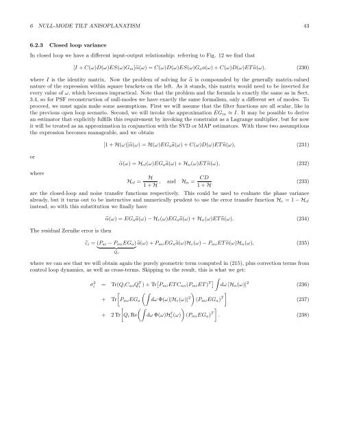
6 NULL-MODE TILT ANISOPLANATISM 436.2.3 Closed loop varianceIn closed loop we have a different input-output relationship: referring to Fig. 12 we find that[I + C(ω)D(ω)ES(ω)G m ]˜α(ω) =C(ω)D(ω)ES(ω)G a a(ω)+C(ω)D(ω)ETñ(ω), (230)where I is the identity matrix. Now the problem of solving for ˜α is compounded by the generally matrix-valuednature of the expression within square brackets on the left. As it stands, this matrix would need to be inverted forevery value of ω, which becomes impractical. Note that the problem and the formula is exactly the same as in Sect.3.4, so for PSF reconstruction of null-modes we have exactly the same formalism, only a different set of modes. Toproceed, we must again make some assumptions. First we will assume that the filter functions are all scalar, like inthe previous open loop scenario. Second, we will invoke the approximation EG m ≈ I. It may be possible to derivean estimator that explicitly fulfills this requirement by invoking the constraint as a Lagrange multiplier, but for nowit will be treated as an approximation in conjunction with the SVD or MAP estimators. With these two assumptionsthe expression becomes manageable, and we obtainor[1 + H(ω)]˜α(ω) =H(ω)EG a ã(ω)+C(ω)D(ω)ETñ(ω), (231)˜α(ω) =H cl (ω)EG a ã(ω)+H n (ω)ETñ(ω), (232)whereH cl =H1+H , and H n = CD(233)1+Hare the closed-loop and noise transfer functions respectively. This could be used to evaluate the phase variancealready, but it turns out to be instructive and numerically prudent to use the error transfer function H ε =1−H clinstead, so with this substitution we finally haveThe residual Zernike error is then˜α(ω) =EG a ã(ω) −H ε (ω)EG a ã(ω)+H n (ω)ETñ(ω). (234)˜ε i =(P ai − P mi EG a )} {{ }ã(ω)+P mi EG a ã(ω)H ε (ω) − P mi ETñ(ω)H n (ω), (235)Q iwhere we can see that we will obtain again the purely geometric term computed in (215), plus correction terms fromcontrol loop dynamics, as well as cross-terms. Skipping to the result, this is what we get:σi 2 = Tr(Q i C aa Q T i )+Tr[ P mi ETC nn (P mi ET) T ] ∫ dω |H n (ω)| 2 (236)(∫)]+ Tr[P mi EG a dω Φ(ω)|H ε (ω)| 2 (P mi EG a ) T (237)[ (∫) ]+ 2Tr Q i Re dω Φ(ω)H ε(ω)† (P mi EG a ) T . (238)