predicting wall temperature with cfd simulations - VolgaSpace.Ru

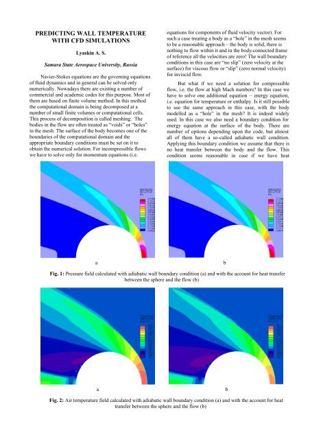
PREDICTING WALL TEMPERATUREWITH CFD SIMULATIONSLyaskin A. S.Samara State Aerospace University, RussiaNavier-Stokes equations are the governing equationsof fluid dynamics and in general can be solved onlynumerically. Nowadays there are existing a number ofcommercial and academic codes for this purpose. Most ofthem are based on finite volume method. In this methodthe computational domain is being decomposed at anumber of small finite volumes or computational cells.This process of decomposition is called meshing. Thebodies in the flow are often treated as “voids” or “holes”in the mesh. The surface of the body becomes one of theboundaries of the computational domain and theappropriate boundary conditions must be set on it toobtain the numerical solution. For incompressible flowswe have to solve only for momentum equations (i.e.equations for components of fluid velocity vector). Forsuch a case treating a body as a “hole” in the mesh seemsto be a reasonable approach – the body is solid, there isnothing to flow within it and in the body-connected frameof reference all the velocities are zero! The wall boundaryconditions in this case are “no slip” (zero velocity at thesurface) for viscous flow or “slip” (zero normal velocity)for inviscid flow.But what if we need a solution for compressibleflow, i.e. the flow at high Mach numbers? In this case wehave to solve one additional equation – energy equation,i.e. equation for temperature or enthalpy. Is it still possibleto use the same approach in this case, with the bodymodelled as a “hole” in the mesh? It is indeed widelyused. In this case we also need a boundary condition forenergy equation at the surface of the body. There arenumber of options depending upon the code, but almostall of them have a so-called adiabatic wall condition.Applying this boundary condition we assume that there isno heat transfer between the body and the flow. Thiscondition seems reasonable in case if we have heatabFig. 1: Pressure field calculated with adiabatic wall boundary condition (a) and with the account for heat transferbetween the sphere and the flow (b)abFig. 2: Air temperature field calculated with adiabatic wall boundary condition (a) and with the account for heattransfer between the sphere and the flow (b)

protection at the surface of the body. And we don’t haveto know anything about the material of the body! But canwe trust the wall temperature distribution obtained withsuch an approach?Modern codes have a capability of solving energyequation both for a fluid flow and for a body (for a solidbody it turns to heat transfer equation). Such a problem iscalled “conjugated heat transfer problem”. For solving thisproblem the body is no longer treated as a “hole” in themesh, it has its own mesh with it. Of course in this casewe have more computational expenses and we have tospecify additional information about the body – thermalconductivity and heat capacity. But with this approach wefields presented at Fig. 2 don’t differ much. But Fig. 3shows the temperature distribution at the surface of thesphere. For the first case the maximum temperature isabout 650°C in the forward stagnation point. And for thesecond case it is about 780°C and it is observed near theequator of the sphere! Though the results of the first caseseem more reasonable from the “common sense” point ofview, the experiment shows that the results of the secondcase are correct. Of course the difference in pressuredistribution will depend upon the material properties – formore “heat resistant” material adiabatic wall boundarycondition will provide more realistic values. But to ensurethe “thermal safety” more sophisticated approaches shouldSolution to conjugatedheat transfer problem“Hall-in-the-mesh”representation for a spherewith adiabatic wall boundaryconditioncan obtain the trustworthy results. And what will be thedifference in the results obtained with these two differentapproaches?Consider the problem of a sphere moving at Mach 3in the air at normal conditions (i.e. atmospheric pressureand t = 20°C). In the first case the sphere as treated as a“hole” in the mesh with adiabatic wall boundaryconditions. In the second case it considered to be made ofstainless steel (with the appropriate values of heat capacityand thermal conductivity) and is meshed together with theflow domain. Note that no special boundary conditions atfluid-solid interface are needed in this case.To solve this problem a commercial code Star-CDwas used. Fig. 1 shows the pressure field for both case (a)and b)). The calculated drag coefficients for both cases arein well agreement with experimental data, as are theshapes of the bow-shock. As it can be seen the differencein flow fields is negligible. Even the flow temperatureFig. 3: Wall temperature calculated with two different approachesbe used.Direct simulation of conjugated heat transferproblem can be too difficult in case of multy-layeredstructures with internal cavities. But there are otherpossibilities. For example, Star-CD offers such option asspecified heat flux through the wall. This allow to run thesimulation with a simple “hole-in-the-mesh” approach,calculating the heat flux through the wall with somesimple tool and correcting the boundary value, say, every100 computational steps. Such an approach yields onlyslight increase of computational expenses and gives muchmore accurate results than using adiabatic wall condition.