NIOSH Method 7400 : Asbestos and Other Fibers by PCM

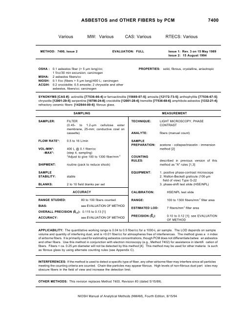
ASBESTOS and OTHER FIBERS by PCM 7400Various MW: Various CAS: Various RTECS: VariousMETHOD: 7400, Issue 2 EVALUATION: FULL Issue 1: Rev. 3 on 15 May 1989Issue 2: 15 August 1994OSHA :MSHA:NIOSH:ACGIH:0.1 asbestos fiber (> 5 µm long)/cc;1 f/cc/30 min excursion; carcinogen2 asbestos fibers/cc0.1 f/cc (fibers > 5 µm long)/400 L; carcinogen0.2 crocidolite; 0.5 amosite; 2 chrysotile and otherasbestos, fibers/cc; carcinogenPROPERTIES: solid, fibrous, crystalline, anisotropicSYNONYMS [CAS #]: actinolite [77536-66-4] or ferroactinolite [15669-07-5]; amosite [12172-73-5]; anthophyllite [77536-67-5];chrysotile [12001-29-5]; serpentine [18786-24-8]; crocidolite [12001-28-4]; tremolite [77536-68-6]; amphibole asbestos [1332-21-4];refractory ceramic fibers [142844-00-6]; fibrous glass.SAMPLINGMEASUREMENTSAMPLER:FILTER(0.45- to 1.2-µm cellulose estermembrane, 25-mm; conductive cowl oncassette)TECHNIQUE:ANALYTE:LIGHT MICROSCOPY, PHASECONTRASTfibers (manual count)FLOW RATE*:VOL-MIN*:-MAX*:SHIPMENT:0.5 to 16 L/min400 L @ 0.1 fiber/cc(step 4, sampling)*Adjust to give 100 to 1300 fiber/mm 2routine (pack to reduce shock)SAMPLEPREPARATION:COUNTINGRULES:acetone - collapse/triacetin - immersionmethod [2]described in previous version of thismethod as "A" rules [1,3]SAMPLESTABILITY:BLANKS:stable2 to 10 field blanks per setEQUIPMENT:1. positive phase-contrast microscope2. Walton-Beckett graticule (100-µmfield of view) Type G-223. phase-shift test slide (HSE/NPL)ACCURACYCALIBRATION:HSE/NPL test slideRANGE STUDIED: 80 to 100 fibers countedBIAS:see EVALUATION OF METHODOVERALL PRECISION (Ŝ rT): 0.115 to 0.13 [1]ACCURACY:see EVALUATION OF METHODRANGE:ESTIMATED LOD:PRECISION (S r):100 to 1300 fibers/mm 2 filter area7 fibers/mm 2 filter area0.10 to 0.12 [1]; see EVALUATIONOF METHODAPPLICABILITY: The quantitative working range is 0.04 to 0.5 fiber/cc for a 1000-L air sample. The LOD depends on samplevolume and quantity of interfering dust, and is

ASBESTOS and OTHER FIBERS by PCM: METHOD 7400, Issue 2, dated 15 August 1994 - Page 2 of 15REAGENTS:1. Acetone,* reagent grade.2. Triacetin (glycerol triacetate), reagent grade.* See SPECIAL PRECAUTIONS.EQUIPMENT:1. Sampler: field monitor, 25-mm, three-piececassette with ca. 50-mm electricallyconductive extension cowl and cellulose esterfilter, 0.45- to 1.2-µm pore size, and backuppad.NOTE 1:Analyze representative filters forfiber background before use tocheck for clarity and background.Discard the filter lot if mean is ≥5fibers per 100 graticule fields.These are defined as laboratoryblanks. Manufacturer-providedquality assurance checks on filterblanks are normally adequate aslong as field blanks are analyzedas described below.NOTE 2: The electrically conductiveextension cowl reduceselectrostatic effects. Ground thecowl when possible duringsampling.NOTE 3:Use 0.8-µm pore size filters forpersonal sampling. The 0.45-µmfilters are recommended forsampling when performing TEManalysis on the same samples.However, their higher pressuredrop precludes their use withpersonal sampling pumps.NOTE 4: Other cassettes have beenproposed that exhibit improveduniformity of fiber deposit on thefilter surface, e.g., bellmouthedsampler (Envirometrics,Charleston, SC). These may beused if shown to give measuredconcentrations equivalent tosampler indicated above for theapplication.2. Personal sampling pump, battery or linepoweredvacuum, of sufficient capacity tomeet flow-rate requirements (see step 4 forflow rate), with flexible connecting tubing.3. Wire, multi-stranded, 22-gauge; 1", hoseclamp to attach wire to cassette.4. Tape, shrink- or adhesive-.5. Slides, glass, frosted-end, pre-cleaned, 25 x75-mm.6. Cover slips, 22- x 22-mm, No. 1-1/2, unlessotherwise specified by microscopemanufacturer.7. Lacquer or nail polish.8. Knife, #10 surgical steel, curved blade.9. Tweezers.NIOSH Manual of Analytical Methods (NMAM), Fourth Edition, 8/15/94

ASBESTOS and OTHER FIBERS by PCM: METHOD 7400, Issue 2, dated 15 August 1994 - Page 3 of 15EQUIPMENT:10. Acetone flash vaporization system for clearingfilters on glass slides (see ref. [5] forspecifications or see manufacturer'sinstructions for equivalent devices).11. Micropipets or syringes, 5-µL and 100- to500-µL.12. Microscope, positive phase (dark) contrast,with green or blue filter, adjustable field iris, 8to 10X eyepiece, and 40 to 45X phaseobjective (total magnification ca. 400X);numerical aperture = 0.65 to 0.75.13. Graticule, Walton-Beckett type with 100-µmdiameter circular field (area = 0.00785 mm 2 ) atthe specimen plane (Type G-22). Availablefrom Optometrics USA, P.O. Box 699, Ayer,MA 01432 [phone (508)-772-1700], andMcCrone Accessories and Components, 850Pasquinelli Drive, Westmont, IL 60559 [phone(312) 887-7100].NOTE: The graticule is custom-made for eachmicroscope. (see APPENDIX A forthe custom-ordering procedure).14. HSE/NPL phase contrast test slide, Mark II.Available from Optometrics USA (addressabove).15. Telescope, ocular phase-ring centering.16. Stage micrometer (0.01-mm divisions).SPECIAL PRECAUTIONS: Acetone is extremely flammable. Take precautions not to ignite it. Heatingof acetone in volumes greater than 1 mL must be done in a ventilated laboratory fume hood using aflameless, spark-free heat source.SAMPLING:1. Calibrate each personal sampling pump with a representative sampler in line.2. To reduce contamination and to hold the cassette tightly together, seal the crease between thecassette base and the cowl with a shrink band or light colored adhesive tape. For personalsampling, fasten the (uncapped) open-face cassette to the worker's lapel. The open face shouldbe oriented downward.NOTE: The cowl should be electrically grounded during area sampling, especially underconditions of low relative humidity. Use a hose clamp to secure one end of the wire(Equipment, Item 3) to the monitor's cowl. Connect the other end to an earth ground(i.e., cold water pipe).3. Submit at least two field blanks (or 10% of the total samples, whichever is greater) for each setof samples. Handle field blanks in a manner representative of actual handling of associatedsamples in the set. Open field blank cassettes at the same time as other cassettes just prior tosampling. Store top covers and cassettes in a clean area (e.g., a closed bag or box) with thetop covers from the sampling cassettes during the sampling period.4. Sample at 0.5 L/min or greater [6]. Adjust sampling flow rate, Q (L/min), and time, t (min), toproduce a fiber density, E, of 100 to 1300 fibers/mm 2 (3.85·10 4 to 5·10 5 fibers per 25-mm filterwith effective collection area A c= 385 mm 2 ) for optimum accuracy. These variables are relatedNIOSH Manual of Analytical Methods (NMAM), Fourth Edition, 8/15/94

ASBESTOS and OTHER FIBERS by PCM: METHOD 7400, Issue 2, dated 15 August 1994 - Page 4 of 15to the action level (one-half the current standard), L (fibers/cc), of the fibrous aerosol beingsampled by:NOTE 1:NOTE 2:The purpose of adjusting sampling times is to obtain optimum fiber loading on thefilter. The collection efficiency does not appear to be a function of flow rate in therange of 0.5 to 16 L/min for asbestos fibers [7]. Relatively large diameter fibers (>3µm) may exhibit significant aspiration loss and inlet deposition. A sampling rate of 1to 4 L/min for 8 h is appropriate in atmospheres containing ca. 0.1 fiber/cc in theabsence of significant amounts of non-asbestos dust. Dusty atmospheres requiresmaller sample volumes ( ≤400 L) to obtain countable samples. In such cases takeshort, consecutive samples and average the results over the total collection time.For documenting episodic exposures, use high flow rates (7 to 16 L/min) overshorter sampling times. In relatively clean atmospheres, where targeted fiberconcentrations are much less than 0.1 fiber/cc, use larger sample volumes (3000 to10000 L) to achieve quantifiable loadings. Take care, however, not to overload thefilter with background dust. If ≥ 50% of the filter surface is covered with particles,the filter may be too overloaded to count and will bias the measured fiberconcentration.OSHA regulations specify a minimum sampling volume of 48 L for an excursionmeasurement, and a maximum sampling rate of 2.5 L/min [3].5. At the end of sampling, replace top cover and end plugs.6. Ship samples with conductive cowl attached in a rigid container with packing material to preventjostling or damage.NOTE: Do not use untreated polystyrene foam in shipping container because electrostaticforces may cause fiber loss from sample filter.SAMPLE PREPARATION:NOTE 1:NOTE 2:The object is to produce samples with a smooth (non-grainy) background in amedium with refractive index ≤1.46. This method collapses the filter for easierfocusing and produces permanent (1 - 10 years) mounts which are useful for qualitycontrol and interlaboratory comparison. The aluminum "hot block" or similar flashvaporization techniques may be used outside the laboratory [2]. Other mountingtechniques meeting the above criteria may also be used (e.g., the laboratory fumehood procedure for generating acetone vapor as described in Method 7400 -revision of 5/15/85, or the non-permanent field mounting technique used in P&CAM239 [3,7,8,9]). Unless the effective filtration area is known, determine the area andrecord the information referenced against the sample ID number [1,9,10,11].Excessive water in the acetone may slow the clearing of the filter, causing materialto be washed off the surface of the filter. Also, filters that have been exposed tohigh humidities prior to clearing may have a grainy background.7. Ensure that the glass slides and cover slips are free of dust and fibers.8. Adjust the rheostat to heat the "hot block" to ca. 70 °C [2].NOTE: If the "hot block" is not used in a fume hood, it must rest on a ceramic plate and beisolated from any surface susceptible to heat damage.9. Mount a wedge cut from the sample filter on a clean glass slide.a. Cut wedges of ca. 25% of the filter area with a curved-blade surgical steel knife using arocking motion to prevent tearing. Place wedge, dust side up, on slide.NOTE: Static electricity will usually keep the wedge on the slide.NIOSH Manual of Analytical Methods (NMAM), Fourth Edition, 8/15/94

ASBESTOS and OTHER FIBERS by PCM: METHOD 7400, Issue 2, dated 15 August 1994 - Page 5 of 15b. Insert slide with wedge into the receiving slot at base of "hot block". Immediately place tipof a micropipet containing ca. 250 µL acetone (use the minimum volume needed toconsistently clear the filter sections) into the inlet port of the PTFE cap on top of the "hotblock" and inject the acetone into the vaporization chamber with a slow, steady pressure onthe plunger button while holding pipet firmly in place. After waiting 3 to 5 sec for the filter toclear, remove pipet and slide from their ports.CAUTION: Although the volume of acetone used is small, use safety precautions. Work ina well-ventilated area (e.g., laboratory fume hood). Take care not to ignite theacetone. Continuous use of this device in an unventilated space may produceexplosive acetone vapor concentrations.c. Using the 5-µL micropipet, immediately place 3.0 to 3.5 µL triacetin on the wedge. Gentlylower a clean cover slip onto the wedge at a slight angle to reduce bubble formation. Avoidexcess pressure and movement of the cover glass.NOTE: If too many bubbles form or the amount of triacetin is insufficient, the cover slip maybecome detached within a few hours. If excessive triacetin remains at the edge ofthe filter under the cover slip, fiber migration may occur.d. Mark the outline of the filter segment with a glass marking pen to aid in microscopicevaluation.e. Glue the edges of the cover slip to the slide using lacquer or nail polish [12]. Counting mayproceed immediately after clearing and mounting are completed.NOTE: If clearing is slow, warm the slide on a hotplate (surface temperature 50 °C) for upto 15 min to hasten clearing. Heat carefully to prevent gas bubble formation.CALIBRATION AND QUALITY CONTROL:10. Microscope adjustments. Follow the manufacturers instructions. At least once daily use thetelescope ocular (or Bertrand lens, for some microscopes) supplied by the manufacturer toensure that the phase rings (annular diaphragm and phase-shifting elements) are concentric.With each microscope, keep a logbook in which to record the dates of microscope cleaningsand major servicing.a. Each time a sample is examined, do the following:(1) Adjust the light source for even illumination across the field of view at the condenseriris. Use Kohler illumination, if available. With some microscopes, the illumination mayhave to be set up with bright field optics rather than phase contract optics.(2) Focus on the particulate material to be examined.(3) Make sure that the field iris is in focus, centered on the sample, and open only enoughto fully illuminate the field of view.b. Check the phase-shift detection limit of the microscope periodically for eachanalyst/microscope combination:(1) Center the HSE/NPL phase-contrast test slide under the phase objective.(2) Bring the blocks of grooved lines into focus in the graticule area.NOTE: The slide contains seven blocks of grooves (ca. 20 grooves per block) indescending order of visibility. For asbestos counting the microscope opticsmust completely resolve the grooved lines in block 3 although they may appearsomewhat faint, and the grooved lines in blocks 6 and 7 must be invisible whencentered in the graticule area. Blocks 4 and 5 must be at least partially visiblebut may vary slightly in visibility between microscopes. A microscope whichfails to meet these requirements has resolution either too low or too high forfiber counting.(3) If image quality deteriorates, clean the microscope optics. If the problem persists,consult the microscope manufacturer.11. Document the laboratory's precision for each counter for replicate fiber counts.a. Maintain as part of the laboratory quality assurance program a set of reference slides to beused on a daily basis [13]. These slides should consist of filter preparations including arange of loadings and background dust levels from a variety of sources including both fieldNIOSH Manual of Analytical Methods (NMAM), Fourth Edition, 8/15/94

ASBESTOS and OTHER FIBERS by PCM: METHOD 7400, Issue 2, dated 15 August 1994 - Page 6 of 15and reference samples (e.g., PAT, AAR, commercial samples). The Quality AssuranceOfficer should maintain custody of the reference slides and should supply each counter witha minimum of one reference slide per workday. Change the labels on the reference slidesperiodically so that the counter does not become familiar with the samples.b. From blind repeat counts on reference slides, estimate the laboratory intra- and intercounterprecision. Obtain separate values of relative standard deviation (S r ) for each sample matrixanalyzed in each of the following ranges: 5 to 20 fibers in 100 graticule fields, >20 to 50fibers in 100 graticule fields, and >50 to 100 fibers in 100 graticule fields. Maintain controlcharts for each of these data files.NOTE: Certain sample matrices (e.g., asbestos cement) have been shown to give poorprecision [9]12. Prepare and count field blanks along with the field samples. Report counts on each field blank.NOTE 1: The identity of blank filters should be unknown to the counter until all counts haveNOTE 2:been completed.If a field blank yields greater than 7 fibers per 100 graticule fields, report possiblecontamination of the samples.13. Perform blind recounts by the same counter on 10% of filters counted (slides relabeled by aperson other than the counter). Use the following test to determine whether a pair of counts bythe same counter on the same filter should be rejected because of possible bias: Discard thesample if the absolute value of the difference between the square roots of the two counts (infiber/mm 2 ) exceeds 2.77 (X)S r ' , where X = average of the square roots of the two fiber counts (infiber/mm 2 ) and S r ' =, where S r is the intracounter relative standard deviation for theappropriate count range (in fibers) determined in step 11. For more complete discussions seereference [13].NOTE 1: Since fiber counting is the measurement of randomly placed fibers which may bedescribed by a Poisson distribution, a square root transformation of the fiber countdata will result in approximately normally distributed data [13].NOTE 2: If a pair of counts is rejected by this test, recount the remaining samples in the setand test the new counts against the first counts. Discard all rejected paired counts.It is not necessary to use this statistic on blank counts.14. The analyst is a critical part of this analytical procedure. Care must be taken to provide a nonstressfuland comfortable environment for fiber counting. An ergonomically designed chairshould be used, with the microscope eyepiece situated at a comfortable height for viewing.External lighting should be set at a level similar to the illumination level in the microscope toreduce eye fatigue. In addition, counters should take 10-to-20 minute breaks from themicroscope every one or two hours to limit fatigue [14]. During these breaks, both eye andupper back/neck exercises should be performed to relieve strain.15. All laboratories engaged in asbestos counting should participate in a proficiency testing programsuch as the AIHA-NIOSH Proficiency Analytical Testing (PAT) Program for asbestos androutinely exchange field samples with other laboratories to compare performance of counters.MEASUREMENT:16. Center the slide on the stage of the calibrated microscope under the objective lens. Focus themicroscope on the plane of the filter.17. Adjust the microscope (Step 10).NOTE: Calibration with the HSE/NPL test slide determines the minimum detectable fiberdiameter (ca. 0.25 µm) [4].18. Counting rules: (same as P&CAM 239 rules [1,10,11]: see examples in APPENDIX B).a. Count any fiber longer than 5 µm which lies entirely within the graticule area.(1) Count only fibers longer than 5 µm. Measure length of curved fibers along the curve.(2) Count only fibers with a length-to-width ratio equal to or greater than 3:1.b. For fibers which cross the boundary of the graticule field:NIOSH Manual of Analytical Methods (NMAM), Fourth Edition, 8/15/94

ASBESTOS and OTHER FIBERS by PCM: METHOD 7400, Issue 2, dated 15 August 1994 - Page 7 of 15(1) Count as 1/2 fiber any fiber with only one end lying within the graticule area, providedthat the fiber meets the criteria of rule a above.(2) Do not count any fiber which crosses the graticule boundary more than once.(3) Reject and do not count all other fibers.c. Count bundles of fibers as one fiber unless individual fibers can be identified by observingboth ends of a fiber.d. Count enough graticule fields to yield 100 fibers. Count a minimum of 20 fields. Stop at100 graticule fields regardless of count.19. Start counting from the tip of the filter wedge and progress along a radial line to the outer edge.Shift up or down on the filter, and continue in the reverse direction. Select graticule fieldsrandomly by looking away from the eyepiece briefly while advancing the mechanical stage.Ensure that, as a minimum, each analysis covers one radial line from the filter center to theouter edge of the filter. When an agglomerate or bubble covers ca. 1/6 or more of the graticulefield, reject the graticule field and select another. Do not report rejected graticule fields in thetotal number counted.NOTE 1: When counting a graticule field, continuously scan a range of focal planes bymoving the fine focus knob to detect very fine fibers which have become embeddedin the filter. The small-diameter fibers will be very faint but are an importantcontribution to the total count. A minimum counting time of 15 seconds per field isappropriate for accurate counting.NOTE 2: This method does not allow for differentiation of fibers based on morphology.Although some experienced counters are capable of selectively counting only fiberswhich appear to be asbestiform, there is presently no accepted method for ensuringuniformity of judgment between laboratories. It is, therefore, incumbent upon alllaboratories using this method to report total fiber counts. If serious contaminationfrom non-asbestos fibers occurs in samples, other techniques such as transmissionelectron microscopy must be used to identify the asbestos fiber fraction present inthe sample (see NIOSH Method 7402). In some cases (i.e., for fibers withdiameters >1 µm), polarized light microscopy (as in NIOSH Method 7403) may beused to identify and eliminate interfering non-crystalline fibers [15].NOTE 3:NOTE 4:NOTE 5:Do not count at edges where filter was cut. Move in at least 1 mm from the edge.Under certain conditions, electrostatic charge may affect the sampling of fibers.These electrostatic effects are most likely to occur when the relative humidity is low(below 20%), and when sampling is performed near the source of aerosol. Theresult is that deposition of fibers on the filter is reduced, especially near the edge ofthe filter. If such a pattern is noted during fiber counting, choose fields as close tothe center of the filter as possible [5].Counts are to be recorded on a data sheet that provides, as a minimum, spaces onwhich to record the counts for each field, filter identification number, analyst's name,date, total fibers counted, total fields counted, average count, fiber density, andcommentary. Average count is calculated by dividing the total fiber count by thenumber of fields observed. Fiber density (fibers/mm 2 ) is defined as the averagecount (fibers/field) divided by the field (graticule) area (mm 2 /field).CALCULATIONS AND REPORTING OF RESULTS20. Calculate and report fiber density on the filter, E (fibers/mm 2 ), by dividing the average fiber countper graticule field, F/n f, minus the mean field blank count per graticule field, B/n b, by thegraticule field area, A f(approx. 0.00785 mm 2 ):NIOSH Manual of Analytical Methods (NMAM), Fourth Edition, 8/15/94

ASBESTOS and OTHER FIBERS by PCM: METHOD 7400, Issue 2, dated 15 August 1994 - Page 8 of 15NOTE: Fiber counts above 1300 fibers/mm 2 and fiber counts from samples with >50% of filterarea covered with particulate should be reported as "uncountable" or "probably biased."Other fiber counts outside the 100-1300 fiber/mm 2 range should be reported as having"greater than optimal variability" and as being "probably biased."21. Calculate and report the concentration, C (fibers/cc), of fibers in the air volume sampled, V (L),using the effective collection area of the filter, A c (approx. 385 mm 2 for a 25-mm filter):NOTE: Periodically check and adjust the value of A c , if necessary.22. Report intralaboratory and interlaboratory relative standard deviations (from Step 11) with eachset of results.NOTE: Precision depends on the total number of fibers counted [1,16]. Relative standarddeviation is documented in references [1,15-17] for fiber counts up to 100 fibers in 100graticule fields. Comparability of interlaboratory results is discussed below. As a firstapproximation, use 213% above and 49% below the count as the upper and lowerconfidence limits for fiber counts greater than 20 (Fig. 1).EVALUATION OF METHOD:A. This method is a revision of P&CAM 239 [10]. A summary of the revisions is as follows:1. Sampling:The change from a 37-mm to a 25-mm filter improves sensitivity for similar air volumes. Thechange in flow rates allows for 2-m 3 full-shift samples to be taken, providing that the filter is notoverloaded with non-fibrous particulates. The collection efficiency of the sampler is not afunction of flow rate in the range 0.5 to 16 L/min [10].2. Sample Preparation Technique:The acetone vapor-triacetin preparation technique is a faster, more permanent mountingtechnique than the dimethyl phthalate/diethyl oxalate method of P&CAM 239 [2,4,10]. Thealuminum "hot block" technique minimizes the amount of acetone needed to prepare eachsample.3. Measurement:a. The Walton-Beckett graticule standardizes the area observed [14,18,19].b. The HSE/NPL test slide standardizes microscope optics for sensitivity to fiber diameter[4,14].c. Because of past inaccuracies associated with low fiber counts, the minimum recommendedloading has been increased to 100 fibers/mm 2 filter area (a total of 78.5 fibers counted in100 fields, each with field area = .00785 mm 2 .) Lower levels generally result in anoverestimate of the fiber count when compared to results in the recommended analyticalrange [20]. The recommended loadings should yield intracounter S rin the range of 0.10 to0.17 [21,22,23].B. Interlaboratory comparability:An international collaborative study involved 16 laboratories using prepared slides from the asbestoscement, milling, mining, textile, and friction material industries [9]. The relative standard deviations(S r) varied with sample type and laboratory. The ranges were:NIOSH Manual of Analytical Methods (NMAM), Fourth Edition, 8/15/94

ASBESTOS and OTHER FIBERS by PCM: METHOD 7400, Issue 2, dated 15 August 1994 - Page 9 of 15Intralaboratory S r Interlaboratory S r Overall S rAIA (NIOSH A Rules)* 0.12 to 0.40 0.27 to 0.85 0.46Modified CRS (NIOSH B Rules)** 0.11 to 0.29 0.20 to 0.35 0.25* Under AIA rules, only fibers having a diameter less than 3 µm are counted and fibers attached toparticles larger than 3 µm are not counted. NIOSH A Rules are otherwise similar to the AIA rules.** See Appendix C.A NIOSH study conducted using field samples of asbestos gave intralaboratory S r in the range 0.17 to0.25 and an interlaboratory S r of 0.45 [21]. This agrees well with other recent studies [9,14,16].At this time, there is no independent means for assessing the overall accuracy of this method. Onemeasure of reliability is to estimate how well the count for a single sample agrees with the mean countfrom a large number of laboratories. The following discussion indicates how this estimation can becarried out based on measurements of the interlaboratory variability, as well as showing how the resultsof this method relate to the theoretically attainable counting precision and to measured intra- andinterlaboratory S r . (NOTE: The following discussion does not include bias estimates and should not betaken to indicated that lightly loaded samples are as accurate as properly loaded ones).Theoretically, the process of counting randomly (Poisson) distributed fibers on a filter surface will givean S r that depends on the number, N, of fibers counted:(1)Thus S r is 0.1 for 100 fibers and 0.32 for 10 fibers counted. The actual Sis greater than these theoretical numbers [17,19,20,21].r found in a number of studiesAn additional component of variability comes primarily from subjective interlaboratory differences. In astudy of ten counters in a continuing sample exchange program, Ogden [15] found this subjectivecomponent of intralaboratory S r to be approximately 0.2 and estimated the overall S r by the term:(2)Ogden found that the 90% confidence interval of the individual intralaboratory counts in relation to themeans were +2 S r and - 1.5 S r . In this program, one sample out of ten was a quality control sample.For laboratories not engaged in an intensive quality assurance program, the subjective component ofvariability can be higher.In a study of field sample results in 46 laboratories, the Asbestos Information Association also found thatthe variability had both a constant component and one that depended on the fiber count [14]. Theseresults gave a subjective interlaboratory component of S r(on the same basis as Ogden's) for fieldsamples of ca. 0.45. A similar value was obtained for 12 laboratories analyzing a set of 24 fieldsamples [21]. This value falls slightly above the range of S r(0.25 to 0.42 for 1984-85) found for 80reference laboratories in the NIOSH PAT program for laboratory-generated samples [17].A number of factors influence S rfor a given laboratory, such as that laboratory's actual countingperformance and the type of samples being analyzed. In the absence of other information, such as froman interlaboratory quality assurance program using field samples, the value for the subjective componentof variability is chosen as 0.45. It is hoped that the laboratories will carry out the recommendedinterlaboratory quality assurance programs to improve their performance and thus reduce the S r.NIOSH Manual of Analytical Methods (NMAM), Fourth Edition, 8/15/94

ASBESTOS and OTHER FIBERS by PCM: METHOD 7400, Issue 2, dated 15 August 1994 - Page 10 of 15The above relative standard deviations apply when the population mean has been determined. It ismore useful, however, for laboratories to estimate the 90% confidence interval on the mean count froma single sample fiber count (Figure 1). These curves assume similar shapes of the count distribution forinterlaboratory and intralaboratory results [16].For example, if a sample yields a count of 24 fibers, Figure 1 indicates that the mean interlaboratorycount will fall within the range of 227% above and 52% below that value 90% of the time. We can applythese percentages directly to the air concentrations as well. If, for instance, this sample (24 fiberscounted) represented a 500-L volume, then the measured concentration is 0.02 fibers/mL (assuming 100fields counted, 25-mm filter, 0.00785 mm 2 counting field area). If this same sample were counted by agroup of laboratories, there is a 90% probability that the mean would fall between 0.01 and 0.08fiber/mL. These limits should be reported in any comparison of results between laboratories.Note that the S r of 0.45 used to derive Figure 1 is used as an estimate for a random group oflaboratories. If several laboratories belonging to a quality assurance group can show that theirinterlaboratory S r is smaller, then it is more correct to use that smaller S r . However, the estimated S r of0.45 is to be used in the absence of such information. Note also that it has been found that S r can behigher for certain types of samples, such as asbestos cement [9].Quite often the estimated airborne concentration from an asbestos analysis is used to compare to aregulatory standard. For instance, if one is trying to show compliance with an 0.5 fiber/mL standardusing a single sample on which 100 fibers have been counted, then Figure 1 indicates that the 0.5fiber/mL standard must be 213% higher than the measured air concentration. This indicates that if onemeasures a fiber concentration of 0.16 fiber/mL (100 fibers counted), then the mean fiber count by agroup of laboratories (of which the compliance laboratory might be one) has a 95% chance of being lessthan 0.5 fibers/mL; i.e., 0.16 + 2.13 x 0.16 = 0.5.It can be seen from Figure 1 that the Poisson component of the variability is not very important unlessthe number of fibers counted is small. Therefore, a further approximation is to simply use +213% and­49% as the upper and lower confidence values of the mean for a 100-fiber count.Figure 1. Interlaboratory Precision of Fiber CountsNIOSH Manual of Analytical Methods (NMAM), Fourth Edition, 8/15/94

ASBESTOS and OTHER FIBERS by PCM: METHOD 7400, Issue 2, dated 15 August 1994 - Page 12 of 15[14] "A Study of the Empirical Precision of Airborne Asbestos Concentration Measurements in theWorkplace by the Membrane Filter Method," Asbestos Information Association, Air MonitoringCommittee Report, Arlington, VA (June, 1983).[15] McCrone, W., L. McCrone and J. Delly, "Polarized Light Microscopy," Ann Arbor Science (1978).[16] Ogden, T. L. "The Reproducibility of Fiber Counts," Health and Safety Executive ResearchPaper 18 (1982).[17] Schlecht, P. C. and S. A. Schulman. "Performance of Asbestos Fiber Counting Laboratories inthe NIOSH Proficiency Analytical Testing (PAT) Program," Am. Ind. Hyg. Assoc. J., 47, 259-266(1986).[18] Chatfield, E. J. Measurement of Asbestos Fiber Concentrations in Workplace Atmospheres,Royal Commission on Matters of Health and Safety Arising from the Use of Asbestos in Ontario,Study No. 9, 180 Dundas Street West, 22nd Floor, Toronto, Ontario, CANADA M5G 1Z8.[19] Walton, W. H. "The Nature, Hazards, and Assessment of Occupational Exposure to AirborneAsbestos Dust: A Review," Ann. Occup. Hyg., 25, 115-247 (1982).[20] Cherrie, J., A.D. Jones, and A.M. Johnston. "The Influence of Fiber Density on the Assessmentof Fiber Concentration Using the membrane filter Method." Am. Ind. Hyg. Assoc. J., 47(8), 465-74 (1986).[21] Baron, P. A. and S. Shulman. "Evaluation of the Magiscan Image Analyzer for Asbestos FiberCounting." Am. Ind. Hyg. Assoc. J., (in press).[22] Taylor, D. G., P. A. Baron, S. A. Shulman and J. W. Carter. "Identification and Counting ofAsbestos Fibers," Am. Ind. Hyg. Assoc. J. 45(2), 84-88 (1984).[23] "Potential Health Hazards of Video Display Terminals," NIOSH Research Report, June 1981.[24] "Reference Methods for Measuring Airborne Man-Made Mineral Fibers (MMMF)," WHO/EUROTechnical Committee for Monitoring an Evaluating Airborne MMMF, World Health Organization,Copenhagen (1985).[25] Criteria for a Recommended Standard...Occupational Exposure to Fibrous Glass, U.S.Department of Health, Education, and Welfare, Publ. (NIOSH) 77-152 (1977).METHOD WRITTEN BY:Paul A. Baron, Ph.D., NIOSH/DPSE.APPENDIX A: CALIBRATION OF THE WALTON-BECKETT GRATICULE:Before ordering the Walton-Beckett graticule, the following calibration must be done to obtain a countingarea (D) 100 µm in diameter at the image plane. The diameter, d c (mm), of the circular counting areaand the disc diameter must be specified when ordering the graticule.1. Insert any available graticule into the eyepiece and focus so that the graticule lines are sharpand clear.2. Set the appropriate interpupillary distance and, if applicable, reset the binocular head adjustmentso that the magnification remains constant.3. Install the 40 to 45X phase objective.4. Place a stage micrometer on the microscope object stage and focus the microscope on thegraduated lines.5. Measure the magnified grid length of the graticule, L o(µm), using the stage micrometer.6. Remove the graticule from the microscope and measure its actual grid length, Lbest be accomplished by using a stage fitted with verniers.a(mm). This can7. Calculate the circle diameter, d c(mm), for the Walton-Beckett graticule:NIOSH Manual of Analytical Methods (NMAM), Fourth Edition, 8/15/94

ASBESTOS and OTHER FIBERS by PCM: METHOD 7400, Issue 2, dated 15 August 1994 - Page 13 of 15(5)Example:If L o= 112 µm, L a= 4.5 mm and D = 100 µm, then d c = 4.02 mm.8. Check the field diameter, D (acceptable range 100 µm ± 2 µm) with a stage micrometer uponreceipt of the graticule from the manufacturer. Determine field area (acceptable range 0.00754mm 2 to 0.00817 mm 2 ).APPENDIX B: COMPARISON OF COUNTING RULES:Figure 2 shows a Walton-Beckett graticule as seen through the microscope. The rules will be discussedas they apply to the labeled objects in the figure.Figure 2. Walton-Beckett graticule with fibers.NIOSH Manual of Analytical Methods (NMAM), Fourth Edition, 8/15/94

ASBESTOS and OTHER FIBERS by PCM: METHOD 7400, Issue 2, dated 15 August 1994 - Page 14 of 15These rules are sometimes referred to as the "A" rules.FIBER COUNTObject Count DISCUSSION1 1 fiber Optically observable asbestos fibers are actually bundles of fine fibrils. Ifthe fibrils seem to be from the same bundle the object is counted as asingle fiber. Note, however, that all objects meeting length and aspect ratiocriteria are counted whether or not they appear to be asbestos.2 2 fiber If fibers meeting the length and aspect ratio criteria (length >5 µm andlength-to-width ratio >3 to 1) overlap, but do not seem to be part of thesame bundle, they are counted as separate fibers.3 1 fiber Although the object has a relatively large diameter (>3 µm), it is counted asfiber under the rules. There is no upper limit on the fiber diameter in thecounting rules. Note that fiber width is measured at the widest compactsection of the object.4 1 fiber Although long fine fibrils may extend from the body of a fiber, these fibrilsare considered part of the fiber if they seem to have originally been part ofthe bundle.5 Do not If the object is ≤5 µm long, it is not counted.count6 1 fiber A fiber partially obscured by a particle is counted as one fiber. If the fiberends emanating from a particle do not seem to be from the same fiber andeach end meets the length and aspect ratio criteria, they are counted asseparate fibers.7 1/2 fiber A fiber which crosses into the graticule area one time is counted as 1/2fiber.8 Do not Ignore fibers that cross the graticulate boundary more than once.count count9 Do not Ignore fibers that lie outside the graticule boundary.countNIOSH Manual of Analytical Methods (NMAM), Fourth Edition, 8/15/94

ASBESTOS and OTHER FIBERS by PCM: METHOD 7400, Issue 2, dated 15 August 1994 - Page 15 of 15APPENDIX C. ALTERNATE COUNTING RULES FOR NON-ASBESTOS FIBERSOther counting rules may be more appropriate for measurement of specific non-asbestos fiber types,such as fibrous glass. These include the "B" rules given below (from NIOSH Method 7400, Revision #2,dated 8/15/87), the World Health Organization reference method for man-made mineral fiber [24], andthe NIOSH fibrous glass criteria document method [25]. The upper diameter limit in these methodsprevents measurements of non-thoracic fibers. It is important to note that the aspect ratio limits includedin these methods vary. NIOSH recommends the use of the 3:1 aspect ratio in counting fibers.It is emphasized that hybridization of different sets of counting rules is not permitted. Report specificallywhich set of counting rules are used with the analytical results."B" COUNTING RULES:1. Count only ends of fibers. Each fiber must be longer than 5 µm and less than 3 µm diameter.2. Count only ends of fibers with a length-to-width ratio equal to or greater than 5:1.3. Count each fiber end which falls within the graticule area as one end, provided that the fiber meetsrules 1 and 2 above. Add split ends to the count as appropriate if the split fiber segment also meetsthe criteria of rules 1 and 2 above.4. Count visibly free ends which meet rules 1 and 2 above when the fiber appears to be attached toanother particle, regardless of the size of the other particle. Count the end of a fiber obscured byanother particle if the particle covering the fiber end is less than 3 µm in diameter.5. Count free ends of fibers emanating from large clumps and bundles up to a maximum of 10 ends (5fibers), provided that each segment meets rules 1 and 2 above.6. Count enough graticule fields to yield 200 ends. Count a minimum of 20 graticule fields. Stop at100 graticule fields, regardless of count.7. Divide total end count by 2 to yield fiber count.APPENDIX D. EQUIVALENT LIMITS OF DETECTION AND QUANTITATIONfiber density on filter* fiber concentration in air, f/ccfibers 400-L air 1000-L airper 100 fields fibers/mm 2 sample sample200 255 0.25 0.10100 127 0.125 0.05LOQ.....80...............102..................0.10..................0.0450 64 0.0625 0.02525 32 0.03 0.012520 25 0.025 0.01010 12.7 0.0125 0.0058 10.2 0.010 0.004LOD......5.5.................7..................0.00675.............0.0027* Assumes 385 mm 2 effective filter collection area, and field area = 0.00785 mm 2 , for relatively "clean"(little particulate aside from fibers) filters.NIOSH Manual of Analytical Methods (NMAM), Fourth Edition, 8/15/94