Research Article Complex Dynamics in a Nonlinear Cobweb Model ...

Hindawi Publishing Corporation
Discrete Dynamics in Nature and Society
Volume 2007, Article ID 29207, 14 pages
doi:10.1155/2007/29207
Research Article
Complex Dynamics in a Nonlinear Cobweb Model for
Real Estate Market
Junhai Ma and Lingling Mu
Received 10 October 2006; Revised 1 April 2007; Accepted 2 July 2007
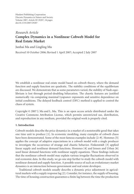
We establish a nonlinear real estate model based on cobweb theory, where the demand
function and supply function are quadratic. The stability conditions of the equilibrium
are discussed. We demonstrate that as some parameters varied, the stability of Nash equilibrium
is lost through period-doubling bifurcation. The chaotic features are justified
numerically via computing maximal Lyapunov exponents and sensitive dependence on
initial conditions. The delayed feedback control (DFC) method is applied to control the
chaos of system.
Copyright © 2007 J. Ma and L. Mu. This is an open access article distributed under the
Creative Commons Attribution License, which permits unrestricted use, distribution,
and reproduction in any medium, provided the original work is properly cited.
1. Introduction
Cobweb models describe the price dynamics in a market of a nonstorable good that takes
onetimeunittoproduce[1]. In economic modeling, many examples of cobweb chaos
have been demonstrated. Some of the most famous examples include [2–9]. Hommes [5]
applies the concept of adaptive expectations in a cobweb model with a single producer
to investigate the occurrence of strange and chaotic behavior. Finkenstädt [3] applied
linear supply and nonlinear demand functions. Hommes [4] and Jensen and Urban [6]
used linear demand functions with nonlinear supply equations. These findings indicate
that the nonlinear cobweb model may explain various irregular fluctuations observed in
real economic data. In this study, we go one step further to study the cobweb model with
nonlinear demand and supply function. A possible source of such an evolutionary market
dynamics is an interaction between government and real estate developer.
Traditional cobweb models usually describe a dynamic price adjustment in agricultural
markets with a supply response lag [2]. Consider, for instance, the supply of housing.
The time of housing construction guarantees a finite lag between the time the production

2 Discrete Dynamics in Nature and Society
decision is made and the time the housing is ready for sale. The real estate developer’s decision
about how many houses should be built and sale is usually based on current and
past experience. This principle is the same as that of agricultural product. So it is feasible
to introduce cobweb model into real estate market.
The present paper attempts to establish a nonlinear model for the real estate market,
and introduce adjustment parameters of housing price and land price into the model,
which can denote the game behavior of players. The system stability with the variation
of parameters is analyzed. Numerical simulations verify the complexity of system evolvement.
Finally, time-delayed feedback control method is used to keep the system from
chaos and bifurcation.
2. Nonlinear models for real estate market
In this paper we assume that all real estate developers in the market are belong to one benefit
group and have a common benefit target. Usually the price p is characterized by the
nonlinear inverse demand function of p = a − b � Q,wherea and b are positive constants,
a is the maximum price in the market, and Q is the total quantity in the market. This kind
of form has been used in other oligopoly models and in the experimental economics dealing
with learning and expectations formation (see, e.g., [10–12]). The transformation of
this formula is as follows:
D1(t) = b0 − b1 p1(t)+b2 p1 2 (t), D2(t) = c0 − c1 p2(t)+c2 p2 2 (t), (2.1)
where b0, b1, b2, c0, c1, c2 are positive constants, p1(t) is the land price at time period t,
p2(t) is the housing price at time period t, D1(t) is the land demand at time period t,
and D2(t) is the housing demand at time period t. Due to the law of demand that the
slope of demand curve is negative, the prices p1(t) andp2(t) must, respectively, satisfy
the inequalies: 2b2 p1(t) − b1 < 0and2c2p2(t) − c1 < 0; 4b2b0 − b 2 1 > 0, 4c2c0 − c 2 1 > 0must
hold, thus the signs of demand equations in formula (2.1) are positive.
In this case, the land market and housing market are interrelated. Though the housing
market does not directly affect land market, the land price impacts the housing supply
which decreases with increasing land price. This rule is the same as that of hog and corn
as stated by Waugh [13]. Real estate companies adjust the housing supply according to
the relative policies and the situation of housing price and land price. The formula of
supply can be supposed as follows:
S1(t) = e0 + e1 p1(t)+e2p1 2 (t), S2(t) = d0 + d1 p2(t)+d2 p2 2 (t) − d3 p1(t), (2.2)
where d0, d1, d2, d3, e0, e1, e2 are positive constants, S1(t)isthelandsupplyattimeperiod
t,andS2(t) is the housing supply at time period t. Because 2e2p1(t)+e1 >0and2d2 p2(t)+
d1 > 0, so we can affirm that the slope of supply curve is positive, and it is in accordance
with the law of supply. Providers begin to supply the products only when
p1(t) > −e1 + � e1 2 − 4e2e0
, p2(t) >
2e2
−d1
�
+
2d2
d1 2 − 4d2d0
. (2.3)

Define
J. Ma and L. Mu 3
Z(p) = D(p) − S(p). (2.4)
Z(p) is excess demand function descending with price, which denotes the gap between
demand and supply. When the price is low, excess demand exists and when the price is
high, excess supply exists, thus p∗ that satisfies the equation Z(p ∗ ) = 0 is called equilibrium
point.
Substituting (2.1)and(2.2)into(2.4), we obtain
Z � p1(t) � = b0 − e0 − � �
e1 + b1 p1(t)+ � �
b2 − e2 p1 2 (t)
Z � p2(t) � = c0 − d0 − � �
d1 + c1 p2(t)+ � �
c2 − d2 p2 2 t = 0,1,2,.... (2.5)
(t)+d3 p1(t),
Since Z(p) follows the law of demand, the following conditions must hold:
b2 − e2 > 0,
c2 − d2 > 0,
2 � �
c2 − d2 p2(t) − � �
d1 + c1 < 0,
2 � �
b2 − e2 p1(t) − � �
e1 + b1 < 0.
(2.6)
α1 is the adjustment parameter of land price, which denotes the adjustment degree of
benchmark land price controlled by government through the land supply plan. α2 is the
adjustment parameter of housing price, the dynamic model of land price and housing
price can be established as follows:
p1(t) = p1(t − 1) + α1Z � p1(t − 1) � ,
p2(t) = p2(t − 1) + α2Z � p2(t − 1) � ,
t = 0,1,2,..., (2.7)
where α1 and α2 are positive parameters.
It is clear that the excess functions of land and housing with adjustment parameters
are two-dimensional nonlinear map, which can be regarded as a discrete dynamic system.
3. Stability analysis
3.1. Bifurcation and chaos. Expansion formula of (2.7)is:
�
p1(t)= p1(t − 1) + α1 b0 − e0 − � �
e1 + b1 p1(t − 1) + � �
b2 − e2 p1 2 (t − 1) � ,
�
p2(t)=p2(t−1)+α2 c0−d0− � �
d1+c1 p2(t−1)+ � �
c2−d2 p2 2 (t−1)+d3p1(t−1) � ,
Let
� �
α1 e2 − b2
u = �
�e1 �2 � �� �
1+α1 + b1 − 4 e0 − b0 e2 − b2
,
U = 1 1
−
2 2 ·
� �
1 − α1 e1 + b1
�
�e1 �2 � �� � , x(t) = up1(t)+U.
1+α1 + b1 − 4 e2 − b2 e0 − b0
t =0,1,2,....
(3.1)
(3.2)

4 Discrete Dynamics in Nature and Society
Thetransformofthefirstequationinformula(3.1) is:
x(t) = λx(t − 1) � 1 − x(t − 1) � , (3.3)
�
where λ = 1+α1 (e1 + b1) 2 − 4(e2 − b2)(e0 − b0). The stability of x(t) variesalongwith
variety of λ according to Logistic rule.
If α1 < 0, then λ

Lemma 3.1. The equilibrium
E1
� b1+e1+
��b1+e1 � � �� �
2−4 e2−b2 e0−b0
2 � � ,
b2−e2
d1+c1+
J. Ma and L. Mu 5
��d1+c1 � � ��
2−4 c2 − d2 c0 − d0 + d3 p1
2 � �
c2 − d2
� �
(3.6)
is an unstable equilibrium point.
Proof. In order to prove this result, we find the eigenvalues of the Jacobian matrix J. In
fact at E1, the Jacobian matrix becomes a triangular matrix:
�
J � E1
⎡
⎢
= ⎣ 1+α1
��b1+e1 �2−4� �� �
e2−b2 e0−b0
�1/2
α2d3
��d1+c1 �2−4� 1+α2
c2−d2
whose eigenvalues are given by the diagonal entries. They are:
�� �2 � �� ��1/2, λ1 = 1+α1 b1 + e1 − 4 e2 − b2 e0 − b0
�� �2 � �� ��1/2. λ2 = 1+α2 d1 + c1 − 4 c2 − d2 c0 − d0 + d3 p1
0
�� c0−d0+d3 p1
⎤
�� ⎥
⎦
1/2
(3.7)
(3.8)
It is clear that when condition (3.5) holds,then|λ1| > 1and|λ2| > 1. Then E1 is an unstable
equilibrium point of the system (3.1). This completes the proof of the proposition.
The stability of other points can also be judged by the above method. �
3.3. The stable region of equilibrium point. In this subsection, we analyze the asymptotic
stability of the equilibrium point for the two-dimensional map (3.1). We determine
the region of stability in the plane of the parameters (α1,α2). The Jacobian matrix at
E ∗ (p1 ∗ (t), p2 ∗ (t)) takes the form
� � � � �
1 − α1 e1 + b1 +2α1 b2 − e2 p1
J =
∗ (t) 0
� � � �
α2d3
1 − α2 d1 + c1 +2α2 c2 − d2 p2 ∗ �
.
(t)
(3.9)
The characteristic equation of the matrix (3.9)hastheform
F(λ) = λ 2 − Tr λ +Det= 0, (3.10)
where “Tr” is the trace and “Det” is the determinant of the Jacobian matrix (3.9) which
are given by
� � � �
Tr = 2 − α1 e1 + b1 +2α1 b2 − e2 p1 ∗ � � � �
(t) − α2 d1 + c1 +2α2 c2 − d2 p2 ∗ (t),
� � � �
Det = 1 − α1 e1 + b1 +2α1 b2 − e2 p1 ∗ � � � �
(t) − α2 d1 + c1 +2α2 c2 − d2 p2 ∗ (t)
+ � � � � �
α1 e1 + b1 − 2α1 b2 − e2 p1 ∗ (t) �� � � � �
α2 d1 + c1 − 2α2 c2 − d2 p2 ∗ (t) � .
(3.11)

6 Discrete Dynamics in Nature and Society
Since
(Tr) 2 −4Det= � � � � � � �
α2 d1+c1 −α1 e1 + b1 +2α1 b2 − e2 p1 ∗ � �
(t) − 2α2 c2 − d2 p2 ∗ (t) �2 > 0,
(3.12)
we deduce that the eigenvalues of equilibrium are real. The local stability of equilibrium
point is given by Jury’s conditions [14, 15] which are as follows.
(a) 1 − Tr + Det > 0.
Lemma 3.2. The condition (a) is always satisfied.
Proof. Because 1 − Tr + Det = [α1(e1 + b1) − 2α1(b2 − e2)p1 ∗ (t)][α2(d1 + c1) − 2α2(c2 −
d2)p2 ∗ (t)], moreover, the last two conditions in (2.6) arehold,α1and α2 are positive
parameters, so the sign of “1 − Tr+Det” is positive and the lemma is proven.
(b) 1 + Tr+Det > 0,
� � � �
1+Tr+Det= 4 − 2α1 e1 + b1 +4α1 b2 − e2 p1 ∗ � � � �
(t) − 2α2 d1 + c1 +4α2 c2 − d2 p2 ∗ (t)
+ � � � � �
α1 e1 + b1 − 2α1 b2 − e2 p1 ∗ (t) �� � � � �
α2 d1 + c1 − 2α2 c2 − d2 p2 ∗ (t) � .
(3.13)
(c) Det−1 < 0,
� � � �
Det−1 =−α1 e1 + b1 +2α1 b2 − e2 p1 ∗ � � � �
(t) − α2 d1 + c1 +2α2 c2 − d2 p2 ∗ (t)
+ � � � � �
α1 e1 + b1 − 2α1 b2 − e2 p1 ∗ (t) �� � � � �
α2 d1 + c1 − 2α2 c2 − d2 p2 ∗ (t) � .
(3.14)
The conditions (b) and (c) define a bounded region of stability in the parameters space
(α1,α2). Then the second and third conditions are the conditions for the local stability of
equilibrium point which becomes
� � � �
1+Tr+Det= 4−2α1 e1 + b1 +4α1 b2 − e2 p1 ∗ � � � �
(t) − 2α2 d1 + c1 +4α2 c2 − d2 p2 ∗ (t)
+ � � � � �
α1 e1 + b1 − 2α1 b2 − e2 p1 ∗ (t) �� � � � �
α2 d1 + c1 − 2α2 c2 − d2 p2 ∗ (t) � >0,
�
Det−1 =−α1 e1 + b1
� � �
+2α1 b2 − e2 p1 ∗ � � � �
(t) − α2 d1 + c1 +2α2 c2 − d2 p2 ∗ (t)
+ � � � � �
α1 e1 + b1 − 2α1 b2 − e2 p1 ∗ (t) �� � � � �
α2 d1 + c1 − 2α2 c2 − d2 p2 ∗ (t) �

α2
0.8
0.6
0.4
0.2
0.5
0.4
0.3
0.2
0.1
4. Numerical simulations
1
0
0 0.4 0.8 1.2 1.6
Figure 3.1. Stability region of Nash equilibrium.
0
0 0.2 0.4 0.6 0.8
α1
Figure 4.1. The graph of map fα1,α2.
J. Ma and L. Mu 7
In order to study the complex dynamics of system (3.1), it is convenient to take the parameters
values as follows:
b0 = 1.2, b1 = 2, b2 = 1.6, c0 = 4, c1 = 1.6, c2 = 0.04, d0 = 0,
d1 = 3, d2 = 0.02, d3 = 0.4, e0 = 0.5, e1 = 0.3, e2 = 0.2.
(4.1)
Figure 3.1 shows the region of stability of Nash equilibrium. Equation (3.15) defines
the region of stability in the plane of (α1,α2). Figure 4.1 shows the map of fα1,α2. xcoordinate
is p1 and y-coordinate is fα1,α2(p1). Dynamics of land price in the cobweb
model is given by system p1(t) = fα1,α2(p1(t − 1)) with two model parameters. A graphical
analysis in Figure 4.1 shows that the map fα1,α2 is nonmonotonic with one critical

8 Discrete Dynamics in Nature and Society
1.2
1
0.8
0.6
0.4
0.2
0.45
0
1.2
1
0.8
0.6
0.4
0.2
0
2
p2
p1
0.5 1 1.5 2 2.5
Lyp
0 0.5 1 1.5 2 2.5
Figure 4.2. Bifurcation diagram for α2 = 0.4.
p2
p1
0.5 1 1.5 2 2.5
Lyp
0 0.5 1 1.5 2 2.5
Figure 4.3. Bifurcation diagram for α2 = 0.2.
point, where the graph has a (local) minimum, and that initial state p1(0) = 1 does not
converge to a low periodic orbit. Since the graphical analysis in this case does not converge,
it suggests that the dynamical behavior is chaotic.
Figures 4.2 and 4.3 show the bifurcation diagrams with respect to the parameter α1
and for α2 = 0.2 and 0.4. In both figures, the Nash equilibrium E ∗ = (0.4,0.9) is locally
stable for small values of the parameter α1. Ifα1 increases, the Nash equilibrium point
α2
α2
α1
α1

p2
p2
0.925
0.92
0.915
0.91
0.905
0.93
0.92
0.91
0.9
0.25 0.5 0.75 1
Figure 4.4. Strange attractor for α2 = 0.07.
p1
0.3 0.6 0.9
Figure 4.5. Strange attractor for α2 = 0.1.
p1
J. Ma and L. Mu 9
becomes unstable, and one observes complex dynamic behavior occurs such as cycles of
higher order and chaos. Also the maximal Lyapunov exponent is plotted in Figures 4.2
and 4.3.
Figures 4.4, 4.5, 4.6, and4.7 show the graph of strange attractors for the different
values of α2.Theparameterα2 takes the values 0.07, 0.1, 0.2, and 0.3, which exhibit fractal
structure in both cases.
We compute the difference of two orbits with initial points [p1(0), p2(0)] and [p1(0) +
0.0001, p2(0)], as well as [p1(0), p2(0)] and [p1(0), p2(0) + 0.0001], to demonstrate the
sensitivity to initial conditions of the system (3.1). The parameters take the values (α1,α2)
= (2.3,0.6) and [p1(0), p2(0)] = (1,2). The results are shown in Figures 4.8 and 4.9,where
Δp1(t) = p1(t) − p ′ 1(t) andp ′ 1(t) isthevalueoflandpriceattimeperiodt with initial

10 Discrete Dynamics in Nature and Society
p2
p2
0.944
0.928
0.912
0.896
1
0.96
0.92
0.88
0.25 0.5 0.75 1
Figure 4.6. Strange attractor for α2 = 0.2.
p1
0.25 0.5 0.75 1
Figure 4.7. Strange attractor for α2 = 0.3.
value of p1(0) + 0.0001; Δp2(t) = p2(t) − p ′ 2(t), and p ′ 2(t) is the value of housing price at
time period t with initial value of p2(0) + 0.0001. In both figures, initial condition of one
coordinate differs by 0.0001, the other coordinate keeps equal. At the beginning, the difference
is indistinguishable but after a number of iterations the difference between them
builds up rapidly. From Figures 4.8 and 4.9, we show that the time series of the system
(3.1) is sensitive dependence on initial conditions, that is, complex dynamics behaviors
occur in this model.
p1

Δp1
Δp2
5. Chaos control
0.8
0.4
0
0.4
0.8
200
100
0
100
200
0 20 40 60 80 100
t
Figure 4.8. Sensitivity to initial conditions of p1.
0 20 40 60 80 100
t
Figure 4.9. Sensitivity to initial conditions of p2.
J. Ma and L. Mu 11
Delay feedback control (DFC) method was brought forward by Pyragas [16]. The method
allows a noninvasive stabilization of unstable periodic orbits (UPOs) of dynamical systems
[17]. It feeds back part of system output signals as exterior input to the system
after a time delay. u(•) is control signal gained by self-feedback coupling between output
and input signals in chaotic system. x(t) = f (x(t − 1)) + u(t) istheformofDFC,where
u(t) = k(x(t) − x(t − τ)), t>τ, τ is time delay, k is controlling factor. Though delay feedback
control is only carried out on one variable, it enables other variables in the system
to achieve stability simultaneously. Our goal is to control the system in such way. The

12 Discrete Dynamics in Nature and Society
p1
1
0.8
0.6
0.4
0.2
2
1.5
1
0.5
0 0.1 0.2 0.3 0.4 0.5
k
Figure 4.10. Relation graph of p1 and k.
0
0 20 40 60 80 100
t
Figure 4.11. Time series of p1 and p2 with k = 0.4.
system with controlling factor is shown as follows:
p1(t) = p1(t − 1) + α1Z � p1(t − 1) � − k � p1(t) − p1(t − τ) � ,
p2(t) = p2(t − 1) + α2Z � p2(t − 1) � ,
p2
p1
t = 0,1,2,.... (5.1)
From Figure 3.1, we know that chaos exists in system (3.1) whenα2 = 0.4, α1 = 2.3.
Choosing τ = 1, first inspect the relation of k and system stability. The Jacobian matrix of

system (5.1)is
�� � � � �
1 − α1 e1 + b1 + k +2α1 b2 − e2 p1(t)
J =
�� (1 + k) 0
� �
α2d3
1−α2 d1+c1 +2α2
J. Ma and L. Mu 13
� c2−d2
�
� .
p2(t)
(5.2)
Substituting equilibrium point (0.4, 0.9) into (5.2), we obtain eigenvalues λ1 =−0.83,
λ2 = (k − 1.7)/(1 + k). So when k>0.35, absolute values of both eigenvalues are less than
1, which means that the system is stable.
As shown in Figure 4.10 land price is controlled from chaotic state to stable state when
k is greater than 0.35, so we select k = 0.4. Housing price and land price are also controlled
to equilibrium point (0.4, 0.9) as shown in Figure 4.11.
6. Conclusion
A nonlinear model for real estate market has been presented based on the cobweb theory.
It is a simple dynamic model with nonlinear demand and supply function. From numerical
simulations, we deduce that the land supply system has the remarkable influence on
real estate market. Therefore, policy makers who intervene in one market should recognize
that what they do may also influence other relative markets. We showed that the
fast adjustment cause a market structure to behave chaotically. Therefore, the dynamics
of market is changed when players apply different adjustment speed. Attempts are also
made to stabilize the chaotic system with the delay feedback method. Combining with
this method, the land price and housing price evolve from chaotic to stable.
Acknowledgments
The authors are grateful to Professor Chen Yu-shu (Academician of Chinese Academy of
Engineering) and Mrs. Liang Jiao-jie for their helpful comments. The authors thank three
anonymous referees for their valuable suggestions and remarks. Any errors or shortcomings
are our own.
References
[1] W. A. Brock and C. H. Hommes, “A rational route to randomness,” Econometrica, vol. 65, no. 5,
pp. 1059–1095, 1997.
[2] C. Chiarella, “The cobweb model, its instability and the onset of chaos,” Economic Modeling,
vol. 5, no. 4, pp. 377–384, 1988.
[3] B. Finkenstädt, Nonlinear Dynamics in Economics: A Theoretical and Statistical Approach to Agricultural
Markets, Lecture Notes in Economics and Mathematical Systems no. 426, Springer,
Berlin, Germany, 1995.
[4] C. H. Hommes, “Adaptive learning and roads to chaos: the case of the cobweb,” Economics Letters,
vol. 36, no. 2, pp. 127–132, 1991.
[5] C. H. Hommes, “Dynamics of the cobweb model with adaptive expectations and nonlinear supply
and demand,” Journal of Economic Behavior & Organization, vol. 24, no. 3, pp. 315–335,
1994.
[6] R. V. Jensen and R. Urban, “Chaotic price behavior in a nonlinear cobweb model,” Economics
Letters, vol. 15, no. 3-4, pp. 235–240, 1984.

14 Discrete Dynamics in Nature and Society
[7] A. Matsumoto, “Ergodic cobweb chaos,” Discrete Dynamics in Nature and Society, vol. 1, no. 2,
pp. 135–146, 1997.
[8] A. Matsumoto, “Preferable disequilibrium in a nonlinear cobweb economy,” Annals of Operations
Research, vol. 89, pp. 101–123, 1999.
[9] H. E. Nusse and C. H. Hommes, “Resolution of chaos with application to a modified Samuelson
model,” Journal of Economic Dynamics & Control, vol. 14, no. 1, pp. 1–19, 1990.
[10] H. N. Agiza, A. S. Hegazi, and A. A. Elsadany, “Complex dynamics and synchronization of a
duopoly game with bounded rationality,” Mathematics and Computers in Simulation, vol. 58,
no. 2, pp. 133–146, 2002.
[11] A. K. Naimzada and L. Sbragia, “Oligopoly games with nonlinear demand and cost functions:
two boundedly rational adjustment processes,” Chaos, Solitons & Fractals, vol.29,no.3,pp.
707–722, 2006.
[12] T. Offerman, J. Potters, and J. Sonnemans, “Imitation and belief learning in an oligopoly experiment,”
Review of Economic Studies, vol. 69, no. 4, pp. 973–997, 2002.
[13] F. V. Waugh, “Cobweb models,” Journal of Farm Economics, vol. 46, no. 4, pp. 732–750, 1964.
[14] T. Puu, Attractors, Bifurcations, and Chaos: Nonlinear Phenomena in Economics, Springer, Berlin,
Germany, 2000.
[15] X. Li, G. Chen, Z. Chen, and Z. Yuan, “Chaotifying linear Elman networks,” IEEE Transactions
on Neural Networks, vol. 13, no. 5, pp. 1193–1199, 2002.
[16] K. Pyragas, “Continuous control of chaos by self-controlling feedback,” Physics Letters A,
vol. 170, no. 6, pp. 421–428, 1992.
[17] V. Pyragas and K. Pyragas, “Delayed feedback control of the Lorenz system: an analytical treatment
at a subcritical Hopf bifurcation,” Physical Review E, vol. 73, no. 3, Article ID 036215, 10
pages, 2006.
Junhai Ma: School of Management, Tianjin University, Tianjin 300072, China
Email address: mjhtju@yahoo.com.cn
Lingling Mu: School of Management, Tianjin University, Tianjin 300072, China
Email address: lingmu1020@163.com

Mathematical Problems in Engineering
Special Issue on
Modeling Experimental Nonlinear Dynamics and
Chaotic Scenarios
Call for Papers
Thinking about nonlinearity in engineering areas, up to the
70s, was focused on intentionally built nonlinear parts in
order to improve the operational characteristics of a device
or system. Keying, saturation, hysteretic phenomena, and
dead zones were added to existing devices increasing their
behavior diversity and precision. In this context, an intrinsic
nonlinearity was treated just as a linear approximation,
around equilibrium points.
Inspired on the rediscovering of the richness of nonlinear
and chaotic phenomena, engineers started using analytical
tools from “Qualitative Theory of Differential Equations,”
allowing more precise analysis and synthesis, in order to
produce new vital products and services. Bifurcation theory,
dynamical systems and chaos started to be part of the
mandatory set of tools for design engineers.
This proposed special edition of the Mathematical Problems
in Engineering aims to provide a picture of the importance
of the bifurcation theory, relating it with nonlinear
and chaotic dynamics for natural and engineered systems.
Ideas of how this dynamics can be captured through precisely
tailored real and numerical experiments and understanding
by the combination of specific tools that associate dynamical
system theory and geometric tools in a very clever, sophisticated,
and at the same time simple and unique analytical
environment are the subject of this issue, allowing new
methods to design high-precision devices and equipment.
Authors should follow the Mathematical Problems in
Engineering manuscript format described at http://www
.hindawi.com/journals/mpe/. Prospective authors should
submit an electronic copy of their complete manuscript
through the journal Manuscript Tracking System at http://
mts.hindawi.com/ according to the following timetable:
Manuscript Due December 1, 2008
First Round of Reviews March 1, 2009
Publication Date June 1, 2009
Hindawi Publishing Corporation
http://www.hindawi.com
Guest Editors
José Roberto Castilho Piqueira, Telecommunication and
Control Engineering Department, Polytechnic School, The
University of São Paulo, 05508-970 São Paulo, Brazil;
piqueira@lac.usp.br
Elbert E. Neher Macau, Laboratório Associado de
Matemática Aplicada e Computação (LAC), Instituto
Nacional de Pesquisas Espaciais (INPE), São Josè dos
Campos, 12227-010 São Paulo, Brazil ; elbert@lac.inpe.br
Celso Grebogi, Center for Applied Dynamics Research,
King’s College, University of Aberdeen, Aberdeen AB24
3UE, UK; grebogi@abdn.ac.uk