Abelian Varieties, 2/9/06 - Notes taken by Kelly McKinnie

Abelian Varieties, 2/9/06 - Notes taken by Kelly McKinnie
March 6, 2006
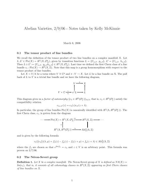
0.1 The tensor product of line bundles
We recall the definition of the tensor product of two line bundles on a complex manifold X. Let
L, L ′ ∈ Pic(X) = H1 (X, O∗ X ), given by transition functions L = {Uα,β, gα,β}, L ′ = {Uα,β, hα,β}.
Then L ⊗ L ′ := {Uα,β, gα,βhα,β} ∈ H1 (X, O∗ X ). Last time we defined the first Chern class of a line
bundle c1 : Pic(X) → H 2 (X, Z). Note that this map is a group homomorphism with respect to the
tensor product of line bundles.
Let X = V/Λ be a torus where V ∼ = C g and π : V → X. Let L be a line bundle on X. The pull
back of L to V is a trivial line bundle and we have the following diagram,
V × C ∼
χ
V��
��
π∗L This diagram gives us a factor of automorphy {eλ ∈ H0 (O∗ V )}λ∈Λ, that is, eλ ∈ H0 (O∗ V ) satisfy the
compatibility relation
π �
� X�
�
��
L
eλ+λ ′(z) = eλ(z)eλ ′(z + λ).
In particular, the group of line bundles Pic(X) is canonically identified with H1 (Λ, H0 (O∗ V )). The
first Chern class, c1, is gotten from the diagram
and is given by the following formula
. . . ��
Pic(X) = H1 (X, O∗ X ) c1 ��
H2 (X, Z)
��
�
H 1 (Λ, H 0 (O ∗ V ))
c1 ��
2
AltZ (Λ, Z)
��
. . .
c1({eλ})(λ, µ) = fλ(z) − fµ(z) − fλ(z + µ) + fµ(z + λ) ∈ Alt 2 Z(Λ, Z)
where the fλ are chosen so that e 2πifλ = eλ and z ∈ V is an arbitrary point. This formula was
proven on 2/7/06.
0.2 The Néron-Severi group
Definition 1. Let X be a complex manifold. The Neron-Severi group of X is defined as NS(X) :=
Im(c1), that is, it consists of all cohomology classes in H 2 (X, Z) appearing as first Chern classes
of line bundles on X.
1

We will describe the Neron-Severi group of a torus. Recall if E = c1(L) where L is a line bundle
on a torus X, then E : Λ × Λ → Z is a Z-alternating form and tensoring this with R we obtain an
R-alternating form E : V × V → R.
Theorem 0.1. For an R-alternating form E : V × V → R, the following are equivalent:
1. E = c1(L) for a line bundle L → X.
2. E(Λ, Λ) ⊆ Z, and E(ix, iy) = E(x, y) for all x, y ∈ V .
Proof. From the short exact sequence of sheaves 0 → Z → OX → O∗ X → 0 we get the following
long exact sequence of cohomology.
· · ·
��
H1 (OX)
��
H1 (O∗ X )
c1 ��
H2 (X, Z)
α ��
H2 (OX)
By definition NS(X) is the kernel of α. By extending scalars from Z to C, where both Z and C are
viewed as constant sheaves, we get the following square, which we are going to show is commutative.
H 2 (X, Z)
α ��
��
H2 (X, C) proj
H 2 (OX)
��
0,2
HDol (X)
The equality on the right hand side is from Dolbeault’s theorem, Hq (Ω p
X
) = Hp,q
Dol (X). The map on
the left hand side of (1) is extension of scalars from Z to C. To see that (1) commutes, we consider
the following morphism of complexes.
0
0
��
C�
�
inc
��
��
OX
��
A 0 X
π proj
��
��
0,0
A
X
d ��
A1 X
¯∂ �
d ��
· · ·
��
� ��
π proj
0,1
AX ¯∂
· · ·
The top row of (2) is used to compute de Rham cohomology, the bottom row of (2) is used to
compute (0, n)-Dolbeault cohomology. This really is a morphism of complexes, that is the squares
commute. We can see this for the second square as follows. Let f ∈ A 0 X .
� ��
��
f(z)
�
d ∂f ∂f
∂z dz + ∂¯z d¯z
��
�
proj
f(z) � ��
∂¯ ∂f ¯ ∂f
= ∂¯z d¯z
The morphism of complexes (2) gives us an induced projection map proj : Hn dR (X) → H(0,n)
Dol (X).
By de Rham’s theorem, H n (X, C) ∼ = H n dR (X), and by Dolbeault’s theorem Hn (OX) ∼ = H (0,n)
Dol (X).
The induced map i : H n (X, C) → H n (OX) is really projection from the Hodge decomposition of
H n (X, C) to H n (OX). The following diagram is commutative.
H n (X, C)
i
��
H n (OX)
∼ ��
Hn dR (X)
∼ �
proj
��
� H 0,n
Dol (X)
Applying this for n = 2 we get that (1) is commutative. To see that the map on the right is really
projection, we first recall the following definitions.
2
��
. . .
(1)
(2)

H q (Ω p
X ) = � p Ω ⊗ � q Ω = H p,q
Dol (X)
where Ω = HomC(V, C) and Ω = HomC−anti(V, C) and
Hn �
dR (X, C) = p+q=n Hp,q (X).
Therefore, H 2 dR (X, C) = � 2 Ω ⊕ (Ω ⊗ Ω) ⊕ � 2 Ω, H 0,2
Dol (X) = � 2 Ω, and the map between them
is really projection. We are now almost done. Let E ∈ H 2 (X, Z) with α(E) = 0. Then write E
in it’s decomposition E = E1 + E2 + E3 with E1 ∈ � 2 Ω, E2 ∈ Ω ⊗ Ω and E3 ∈ � 2 Ω. By the
commutativity of (1) α(E) = E3, and therefore E3 = 0.
Exercise 0.2. Let E : V × V → C an R alternating form. Show E(V × V ) ⊆ R if and only if
E1 = E3.
This exercise implies that E1 = E3 = 0, and therefore, E = E2, that is, it is a (1,1) form. The
(1,1)-forms are precisely those that satisfy E(ix, iy) = E(x, y). To see this, let f ⊗ g ∈ Ω ⊗ Ω, a
simple tensor, where f : V → C is C-linear and g : V → C is C-anti-linear. We now check that
f ⊗ g(ix, iy) = f ⊗ g(x, y):
f ⊗ g(ix, iy) = f(ix)g(iy)
= if(x)(−i)g(y)
= f(x)g(y) = f ⊗ g(x, y)
Exercise 0.3. Show Ω ⊗ Ω = {E : V × V → C | E(ix, iy) = E(x, y)}. Just above we proved “⊆”.
To prove the other inclusion count dimensions.
With this the theorem has been proved.
Corollary 0.4. There exists a bijection between NS(X) and the space of Hermitian forms H :
V × V → C such that ImH(Λ, Λ) ⊆ Z.
Recall a form is said to be Hermitian if it is C-linear and H(x, y) = H(y, x).
Proof. By Theorem 0.1, NS(X) = {E : V × V → R, alternating | E(Λ, Λ) ⊆ Z, with E(ix, iy) =
E(x, y)}. The bijection takes
E ↦→ H : V × V → C
where H(x, y) = E(ix, y) + iE(x, y). We need to check that this is a Hermitian form:
0.3 The Appell-Humbert Theorem
H(y, x) = E(iy, x) − iE(y, x) = −E(y, ix) − iE(y, x)
= E(ix, y) + iE(x, y) = H(x, y)
The Appell-Humbert Theorem was proved by Appell and Humbert in the 1890’s for dimension 2.
It was proved by Lefschetz in general. It is the most important theorem so far in the class. Recall
our general set up, L → X = V/Λ, a line bundle. From L we get factors of automorphy {eλ}.
We would like to get a canonical factor of automorphy representing L, that is, a distinguished
representative.
Definition 2. A semi-character for H ∈ NS(X) is a map χ : Λ → S 1 = {z ∈ C | |z| = 1} such
that
χ(λ + λ ′ ) = χ(λ)χ(λ ′ )e πiE(λ,λ′ ) .
3
(3)

Example: H = 0; the semi-characters for 0 are Hom(Λ, S 1 ).
Definition 3. P(Λ) = {(H, χ) | H ∈ NS(X), χ is a semi-character for H}.
P(Λ) is a group with operation (H1, χ1)(H2, χ2) = (H1 + H2, χ1χ2). There exists an exact
sequence
1 ��
Hom(Λ, S1 p
) ��
P(Λ) ��
NS(X).
p is the “forget the semi-character” map. It is not clear yet that p is surjective, but it will be true.
In fact, we will eventually have Pic(X) ∼ = P(Λ), where the map is defined as follows.
P(Λ)
a ��
Pic(X) ∼
can ��
H1 (Λ, H0 (O∗ V )) (factors of automorphy)
(H, χ) � a ��
L(H, χ)
where a(H, χ) = L(H, χ) is the line bundle given by the factors of automorphy
π
πH(z,λ)+
a(H, χ) = {aλ(z) = χ(λ)e 2 H(λ,λ) }λ ∈ H 0 (O ∗ V ).
We need to show that this definition makes {aλ} into a factor of automorphy, that is, we need to
show that aλ+λ ′(z) = aλ(z)aλ ′(z + λ):
aλ+λ ′(z) = χ(λ + λ′ )e πH(z,λ+λ′ )+ π
2 H(λ+λ′ ,λ+λ ′ )
= χ(λ)χ(λ ′ )e πiE(λ,λ′ ) e πH(z,λ ′ )+πH(z,λ)+ π
2 [H(λ,λ)+H(λ′ ,λ ′ )+H(λ,λ ′ )+H(λ ′ ,λ)]
�
= χ(λ)e
�
= χ(λ)e
π
πH(z,λ)+ 2
π
πH(z,λ)+ 2
= aλ(z)aλ ′(z + λ)
H(λ,λ)� �
χ(λ ′ )e πH(z,λ′ )+ π
2 H(λ′ ,λ ′ ) e πiE(λ,λ ′ )+πRe(H(λ,λ ′ )) �
H(λ,λ)� �
χ(λ ′ )e πH(z+λ,λ′ )+ π
2 H(λ′ ,λ ′ ) �
The 4-th equality follows from the relation H(x, y) = E(ix, y) + iE(x, y).
The Appell-Humbert Theorem says that a : P(Λ) → Pic(X) is an isomorphism. We will prove
this next time. This gives a geometric description of what all line bundles look like. Because, as a
total space, we have:
L(H, χ) = V × C/ ∼
where (z, t) ∼ (z + λ, aλ(z)t).
Proposition 0.5. The diagram
��
��
�
P(Λ)
����
�p
����
a
Pic(X)
c1
���������� NS(X)
is commutative where p is the “forget the semi-character” map. In particular, c1(L(H, χ)) = H.
4