Ch 9 Interval Estimation

Ch 9. Interval Estimation 

Intro 

Chapter 9 

Intro 

Finding Interval 

Estimator 

Optimal theory 

for CI 

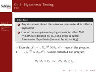
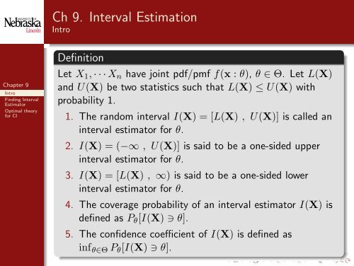
Definition 

Let X 1 , · · · X n have joint pdf/pmf f(x : θ), θ ∈ Θ. Let L(X) 

and U(X) be two statistics such that L(X) ≤ U(X) with 

probability 1. 

1. The random interval I(X) = [L(X) , U(X)] is called an 

interval estimator for θ. 

2. I(X) = (−∞ , U(X)] is said to be a one-sided upper 


3. I(X) = [L(X) , ∞) is said to be a one-sided lower 


4. The coverage probability of an interval estimator I(X) is 

defined as P θ [I(X) ∋ θ]. 

5. The confidence coefficient of I(X) is defined as 

inf θ∈Θ P θ [I(X) ∋ θ].


Intro 


Intro 


Estimator 


for CI 

⊲ Example: X 1 , · · · , X n 

iid 

∼ Uniform(0, θ). Consider the 

following two interval estimator of θ. 

I 1 (X) = [aX (n) , bX (n) ], 1 ≤ a < b 

I 2 (X) = [X (n) + c , ∞)


Finding Interval Estimator - Inverting test 

⊲ Example: X 1 , · · · , X n 

iid 

∼ N(θ, 1) 


Intro 


Estimator 


for CI 

H 0 : θ = θ 0 vs H 1 : θ ≠ θ 0 

The LRT of size α is 

{ 

1, | √ n(¯x − θ 0 )| ≥ z 

φ(x) = 

1−α/2 , 

0, elsewhere. 

=⇒ P θ0 { ¯X − z 1−α/2 / √ n ≤ θ 0 ≤ ¯X + z 1−α/2 / √ n} =




Intro 


Estimator 


for CI 

Theorem 

Let X 1 , · · · , X n have joint pdf/pmf f(x : θ), θ ∈ Θ. For each 

θ 0 ∈ Θ, let A(θ 0 ) denote the acceptance region of a size α 

simple test for testing 

H 0 : θ = θ 0 vs H 1 : θ ≠ θ 0 

Define a set C(x) = {θ 0 ∈ Θ : x ∈ A(θ 0 )}. Then C(X) is a 

confidence set with confidence coefficient 1 − α. 

⊳ Note: 

1. C(X) is not necessarily an interval. 

2. One may need to consider one-sided test for one-sided 

confidence interval.




Intro 


Estimator 


for CI 

⊲ Example: X 1 , · · · , X n 

iid 

∼ N(µ, σ 2 ). µ and σ 2 are unknown. 

Find a 1 − α two-sided CI and on e-sided lower CI for µ.




Intro 


Estimator 


for CI 

⊲ Example: X 1 , · · · , X n 

iid 

∼ f(x|θ) = θ 2 xe −θx , x > 0. Find an 

approximate 1 − α confidence set of θ


Finding Interval Estimator - Using PQ 


Intro 


Estimator 


for CI 

Definition 

Let X 1 , · · · , X n have joint pdf/pmf f(x : θ), θ ∈ Θ. A random 

variable Y = Q(X : θ) is called a pivotal quantity (PQ) if the 

distribution of Y = Q(X : θ) does not depend on θ. 

⊲ Example: X 1 , · · · , X n 

iid 

∼ f(x : θ). Consider the following 

families of distributions and statistics. 

1. f(x : θ) = f 0 (x − θ) 

2. f(x : θ) = 1 θ f 0(x) 

3. f(x : θ) = 1 θ 2 

f 0 [(x − θ 1 )/θ 2 ] 

¯X n − θ, ¯Xn /θ, ( ¯X n − θ 1 )/θ 2




Intro 


Estimator 


for CI 

⊲ Example: X 1 , · · · , X n 

iid 

∼ exp(λ). 

T = ∑ X i ∼ Gamma( , ) 

Find a (1 − α)% confidence interval of λ.




Intro 


Estimator 


for CI 

Theorem (See the theorem 2.1.10 for reference) 

Suppose T = T (X) is a statistic calculated from X 1 , · · · , X n . 

Assume T has a continuous distribution with cdf 

F (t : θ) = P θ (T ≤ t). 

Then 

Q(T : θ) = F (T : θ) 

is a PQ. 

⊳ Note: In order for Q(T : θ) = F (T : θ) to result in a 

confidence interval, we want F (T : θ) to be monotone in θ. A 

cdf F (T : θ) that is increasing or decreasing in θ for all t is said 

to be stochastically increasing or decreasing.




Intro 


Estimator 


for CI 

iid 

⊲ Example: X 1 , · · · , X n ∼ N(µ, σ 2 ), σ 2 is known. Let 

T (X) = ¯X. Then 

( ) T − µ 

Q(T : µ) = F (T : µ) = Φ 

σ/ √ . 

n




Intro 


Estimator 


for CI 

iid 

⊲ Example: X 1 , · · · , X n ∼ f(x : µ) = e −(x−µ) , x ≥ µ. Let 

T (X) = X (1) = min 1≤i≤n X i . Derive (1 − α)100% confidence 

interval using the cdf of T .


Finding Interval Estimator - Bayesian Interval 


Intro 


Estimator 


for CI 

Definition 

[L(x), U(x)] is called a (1 − α)100% credible set (or Bayesian 

interval) if 

1 − α = P [L(x) < θ < U(x)|X = x] 

{ ∑ 

θ 

π(θ|x) discrete 

= ∫ 

θ π(θ|x)dθ continuous 

⊲ Example: X 1 , · · · , X n 

iid 

∼ N(µ, 1). µ ∼ N(0, 1). Find a 

(1 − α) credible set.


Optimal theory for CI 

CI: Length of CI vs Coverage probability 


Intro 


Estimator 


for CI 

Definition 

f(x) is a unimodal pdf if f(x) is nondecreasing for x ≤ x ∗ and 

nonincreasing for x ≥ x ∗ in which case x ∗ is the mode of the 

distribution. 

Theorem (Shortest CI based on unimodal distn.) 

Let f(x) be a unimodal pdf. If the interval [a, b] satisfies 

i. ∫ b 

a f(x)dx = 1 − α 

ii. f(a) = f(b) > 0 

iii. a ≤ x ∗ ≤ b, when x ∗ is a mode of f(x) 

Then no other interval estimator satisfying (i) is shorter than 

[a, b].




Intro 


Estimator 


for CI 

⊲ Example: X 1 , · · · , X n 

iid 

∼ N(µ, σ 2 ). σ 2 is known. 

⊲ Example: X 1 , · · · , X n 

iid 

∼ N(µ, σ 2 ). σ 2 is unknown.




Intro 


Estimator 


for CI 

Definition (Probability of false coverage) 

For θ ′ ≠ θ, P θ [L(X) ≤ θ ′ ≤ U(X)] 

For θ ′ < θ, P θ [L(X) ≤ θ ′ ] 

For θ ′ > θ, P θ [θ ′ ≤ U(X)] 

Definition 

A 1 − α confidence interval with minimum probability of false 

coverage is called a Uniformly Most Accurate (UMA) 1 − α 

confidence interval.




Intro 


Estimator 


for CI 

Theorem (UMA CI based on UMP test) 

Let X 1 , · · · , X n have a joint pdf/pmf f(x : θ). Suppose that a 

UMP test of size α for testing H 0 : θ ≤ θ 0 vs H 1 : θ > θ 0 

exists and given as 

{ 

φ(x) = 

1, x /∈ A ∗ (θ 0 ), 

0, x ∈ A ∗ (θ 0 ). 

Let C ∗ (X) be the confidence interval obtained by inverting the 

UMP acceptance region. Then, for any other 1 − α confidence 

region(set, interval), 

P θ [θ ′ ∈ C ∗ (X)] ≤ P θ [θ ′ ∈ C ∗ (X)], 

for all θ ′ < θ. That is, inverting UMP test yields a UMA 

confidence region(set, interval).




Intro 


Estimator 


for CI 

⊳ Note: UMP unbiased test can be inverted to obtain UMA 

unbiased confidence region(set, interval). 

⊲ Example: X 1 , · · · , X n 

iid 

∼ N(µ, σ 2 ). σ 2 is known.

Ch 9 Interval Estimation

You also want an ePaper? Increase the reach of your titles

Delete template?

Save as template?