Applications of nonlinear diffusion in image processing and
Applications of nonlinear diffusion in image processing and
Applications of nonlinear diffusion in image processing and

Create successful ePaper yourself
Turn your PDF publications into a flip-book with our unique Google optimized e-Paper software.
Acta Math. Univ. Comenianae<br />
Vol. LXX, 1(2001), pp. 33–50<br />
Proceed<strong>in</strong>gs <strong>of</strong> Algoritmy 2000<br />
APPLICATIONS OF NONLINEAR DIFFUSION IN<br />
IMAGE PROCESSING AND COMPUTER VISION<br />
J. WEICKERT<br />
Abstract. Nonl<strong>in</strong>ear <strong>diffusion</strong> processes can be found <strong>in</strong> many recent methods<br />
for <strong>image</strong> process<strong>in</strong>g <strong>and</strong>computer vision. In this article, four applications are<br />
surveyed: <strong>nonl<strong>in</strong>ear</strong> <strong>diffusion</strong> filter<strong>in</strong>g, variational <strong>image</strong> regularization, optic flow<br />
estimation, <strong>and</strong>geodesic active contours. For each <strong>of</strong> these techniques we expla<strong>in</strong><br />
the ma<strong>in</strong> ideas, discuss theoretical properties <strong>and</strong> present an appropriate numerical<br />
scheme. The numerical schemes are based on additive operator splitt<strong>in</strong>gs (AOS).<br />
In contrast to traditional multiplicative splitt<strong>in</strong>gs such as ADI, LOD or D’yakonov<br />
splitt<strong>in</strong>gs, all axes are treated <strong>in</strong> the same manner, <strong>and</strong> additional possibilities<br />
for efficient realizations on parallel <strong>and</strong>distributedarchitectures appear. Geodesic<br />
active contours leadto equations that resemble mean curvature motion. For this<br />
application, a novel AOS scheme is presentedthat uses harmonic averag<strong>in</strong>g <strong>and</strong><br />
does not require re<strong>in</strong>itializations <strong>of</strong> the distance function <strong>in</strong> each iteration step. Its<br />
accuracy is evaluated<strong>in</strong> case <strong>of</strong> mean curvature motion.<br />
1. Introduction<br />
Many mathematicians have been attracted by <strong>image</strong> process<strong>in</strong>g <strong>and</strong> computer<br />
vision <strong>in</strong> recent years. This has been triggered by mathematically well-founded<br />
methods us<strong>in</strong>g e.g. wavelets or <strong>nonl<strong>in</strong>ear</strong> partial differential equations. The goal<br />
<strong>of</strong> the present paper is to give an <strong>in</strong>troduction to a subarea <strong>of</strong> this field, namely<br />
methods that are based on <strong>nonl<strong>in</strong>ear</strong> <strong>diffusion</strong> techniques.<br />
This field has evolved <strong>in</strong> a very fruitful way. It is closely connected to a specific<br />
k<strong>in</strong>d <strong>of</strong> multiscale analysis called scale-space [23, 32], <strong>and</strong> it has first been used<br />
for <strong>image</strong> smooth<strong>in</strong>g with simultaneous edge enhancement [26]. Later on, close<br />
connections to regularization methods have been discovered [29], <strong>and</strong> related <strong>nonl<strong>in</strong>ear</strong><br />
methods have also entered computer vision fields such as motion analysis<br />
<strong>in</strong> <strong>image</strong> sequences [8] or <strong>in</strong>teractive segmentation [4, 20]. In this paper we shall<br />
learn about the basic ideas beh<strong>in</strong>d these methods, but also about their theoretical<br />
foundation <strong>and</strong> their adequate numerical realization.<br />
In this context we will also discuss the specific requirements for adequate numerical<br />
schemes <strong>in</strong> <strong>image</strong> process<strong>in</strong>g or computer vision. Among the variety <strong>of</strong><br />
ReceivedJanuary 10, 2001.<br />
2000 Mathematics Subject Classification. Primary 35-K35, 65-M06, 68-W10, 94-A08.<br />
Key words <strong>and</strong> phrases. Nonl<strong>in</strong>ear <strong>diffusion</strong>, variational methods, <strong>image</strong> process<strong>in</strong>g, computer<br />
vision, f<strong>in</strong>ite difference methods, parallel algorithms, mean curvature motion.<br />
33
34 J. WEICKERT<br />
numerical methods that fulfill these requirements, we focus on a specific class <strong>of</strong><br />
splitt<strong>in</strong>g-based f<strong>in</strong>ite difference schemes. These semi-implicit schemes differ from<br />
their classical counterparts by the fact that they use additive operator splitt<strong>in</strong>gs<br />
(AOS) <strong>in</strong>stead <strong>of</strong> multiplicative ones. It will be shown that these AOS schemes<br />
are simple <strong>and</strong> efficient, do not require additional parameters, <strong>in</strong>herit important<br />
properties from the cont<strong>in</strong>uous equations, <strong>and</strong> are widely applicable.<br />
The paper is organized as follows: Section 2 gives an <strong>in</strong>troduction to <strong>nonl<strong>in</strong>ear</strong><br />
<strong>diffusion</strong> filter<strong>in</strong>g, while Section 3 describes its relation to regularization methods.<br />
In Section 4, <strong>nonl<strong>in</strong>ear</strong> <strong>diffusion</strong> is used for analys<strong>in</strong>g motion <strong>in</strong> <strong>image</strong> sequences,<br />
<strong>and</strong> Section 5 shows how <strong>diffusion</strong>-like ideas can be used for <strong>in</strong>teractive segmentation.<br />
Each <strong>of</strong> these sections expla<strong>in</strong>s the ma<strong>in</strong> ideas, the theoretical foundation <strong>of</strong><br />
the method, <strong>and</strong> an appropriate numerical realization <strong>in</strong> terms <strong>of</strong> AOS schemes.<br />
While sections 2–4 survey work that has been published elsewhere, a novel AOS<br />
scheme for mean curvature motion <strong>and</strong> geodesic active contours is <strong>in</strong>troduced <strong>in</strong><br />
Section 5.<br />
Related work. In view <strong>of</strong> the large amout <strong>of</strong> publications <strong>in</strong> this area, we have<br />
to refer the reader to some recent collections <strong>and</strong> books <strong>in</strong> order to obta<strong>in</strong> a more<br />
detailed overview <strong>of</strong> the state-<strong>of</strong>-the-art <strong>in</strong> <strong>diffusion</strong>-based <strong>image</strong> process<strong>in</strong>g [5, 23,<br />
32, 34]. Compared to this large number <strong>of</strong> publications, however, the number <strong>of</strong><br />
papers deal<strong>in</strong>g with numerical aspects <strong>of</strong> <strong>diffusion</strong> filter<strong>in</strong>g is still relatively small.<br />
S<strong>in</strong>ce the pixel structure <strong>of</strong> digital <strong>image</strong>s provides a natural discretization on a<br />
fixed rectangular grid, it is not surpris<strong>in</strong>g that <strong>of</strong>ten f<strong>in</strong>ite difference methods are<br />
used <strong>in</strong> the <strong>image</strong> process<strong>in</strong>g community. For simplicity reasons, explicit schemes<br />
are still very common, but absolutely stable semi-implicit schemes [6, 13, 39] are<br />
becom<strong>in</strong>g more <strong>and</strong> more popular. Alternatives to f<strong>in</strong>ite differences <strong>in</strong>clude f<strong>in</strong>ite<br />
element methods [3, 19, 27, 30], wavelets [10, 11], f<strong>in</strong>ite <strong>and</strong> complementary<br />
volume schemes [13], pseudospectral approaches [11], lattice Boltzmann methods<br />
[17], <strong>and</strong> stochastic simulations [28].<br />
2. Nonl<strong>in</strong>ear Diffusion Filter<strong>in</strong>g<br />
2.1. Basic Idea<br />
Nonl<strong>in</strong>ear <strong>diffusion</strong> filter<strong>in</strong>g goes back to Perona <strong>and</strong> Malik [26]. Although their<br />
method <strong>in</strong> its orig<strong>in</strong>al formulation is regarded to be ill-posed, it has triggered a lot<br />
<strong>of</strong> research; see [33, 34] for overviews. In the follow<strong>in</strong>g we shall be concerned with<br />
one <strong>of</strong> its earliest regularizations that is due to Catté, Lions, Morel, <strong>and</strong> Coll [6].<br />
Let Ω := (0,a1) ×·×(0,am) be our <strong>image</strong> doma<strong>in</strong> <strong>in</strong> Rm <strong>and</strong> consider a<br />
(scalar) <strong>image</strong> f(x) ∈ L∞ (Ω). Then a filtered <strong>image</strong> u(x, t) <strong>of</strong>f(x) iscalculated<br />
by solv<strong>in</strong>g a <strong>nonl<strong>in</strong>ear</strong> <strong>diffusion</strong> equation with the orig<strong>in</strong>al <strong>image</strong> as <strong>in</strong>itial state,<br />
<strong>and</strong> homogeneous Neumann boundary conditions:<br />
(1) ∂tu = div � g(|∇uσ| 2 ) ∇u �<br />
on Ω × (0, ∞),
(2)<br />
(3)<br />
DIFFUSION IN COMPOTER VISION 35<br />
u(x, 0) = f(x) on Ω,<br />
∂nu = 0 on ∂Ω × (0, ∞),<br />
where n denotes the normal to the <strong>image</strong> boundary ∂Ω.<br />
The “time” t is a scale parameter: larger values lead to simpler <strong>image</strong> representations.<br />
In order to reduce smooth<strong>in</strong>g at edges, the diffusivity g is chosen as<br />
a decreas<strong>in</strong>g function <strong>of</strong> the edge detector |∇uσ| 2 ,where∇uσ is the gradient <strong>of</strong> a<br />
Gaussian-smoothed version <strong>of</strong> u:<br />
(4)<br />
(5)<br />
We use the diffusivity<br />
∇uσ := ∇(Kσ ∗ u),<br />
Kσ :=<br />
(6) g(s 2 ) :=<br />
1<br />
(2πσ2 exp<br />
) m/2<br />
�<br />
− |x|2<br />
2σ2 �<br />
.<br />
�<br />
1<br />
�<br />
2 (s=0) 1 − exp (s2 > 0).<br />
� −c<br />
(s/λ) 8<br />
For such rapidly decreas<strong>in</strong>g diffusivities, smooth<strong>in</strong>g on both sides <strong>of</strong> an edge is<br />
much stronger than smooth<strong>in</strong>g across it. This selective smooth<strong>in</strong>g process prefers<br />
<strong>in</strong>traregional smooth<strong>in</strong>g to <strong>in</strong>terregional blurr<strong>in</strong>g. One can ensure that the flux<br />
Φ(s) :=sg(s 2 ) is <strong>in</strong>creas<strong>in</strong>g for |s| ≤λ <strong>and</strong> decreas<strong>in</strong>g for |s| >λby choos<strong>in</strong>g<br />
c ≈ 3.315. Thus, λ is a contrast parameter separat<strong>in</strong>g low-contrast regions with<br />
(smooth<strong>in</strong>g) forward <strong>diffusion</strong> from high-contrast locations where backward <strong>diffusion</strong><br />
may enhance edges [26]. Other choices <strong>of</strong> diffusivities are possible as well, but<br />
experiments <strong>in</strong>dicated that (6) may lead to more segmentation-like results than<br />
the functions used <strong>in</strong> [26].<br />
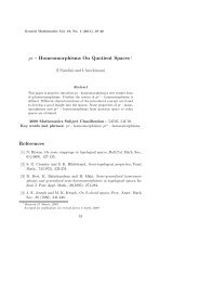
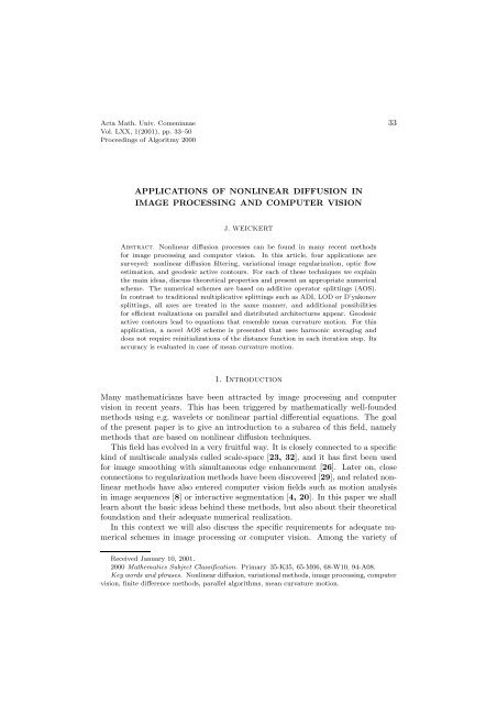
Figure 1 shows an application <strong>of</strong> <strong>image</strong> restoration by means <strong>of</strong> such a forwardbackward<br />
<strong>diffusion</strong> filter. A mammogram is denoised <strong>in</strong> such a way that the<br />
diagnostically relevant microcalcifications become much better visible.<br />
2.2. Theoretical Foundation<br />
2.2.1. Cont<strong>in</strong>uous Formulation. The preced<strong>in</strong>g <strong>nonl<strong>in</strong>ear</strong> <strong>diffusion</strong> filter belongs<br />
to a much larger filter class for which useful theoretical properties can be<br />
established. In particular it is possible to replace the scalar-valued diffusivity g<br />
by a smooth matrix-valued function D that rema<strong>in</strong>s uniformly positive def<strong>in</strong>ite as<br />
long as its argument is bounded. This allows for more flexible <strong>nonl<strong>in</strong>ear</strong> <strong>diffusion</strong><br />
models [34]. For such a class the follow<strong>in</strong>g properties can be established.<br />
(a) (Well-posedness <strong>and</strong> smoothness results)<br />
There exists a unique solution u(x, t) <strong>in</strong> the distributional sense which is <strong>in</strong><br />
C∞ ( ¯ Ω × (0, ∞)) <strong>and</strong> depends cont<strong>in</strong>uously on f with respect to the L2 (Ω)<br />
norm.<br />
(b) (Extremum pr<strong>in</strong>ciple)<br />
Let a := <strong>in</strong>fΩ f <strong>and</strong> b := supΩ f. Then, a ≤ u(x, t) ≤ b on Ω × [0, ∞).
36 J. WEICKERT<br />
Figure 1. (a) Top Left: Mammogram with six microcalcifications, Ω = (0, 128) 2 . (b) Top<br />
Right: 3D plot <strong>of</strong> (a), where the graph <strong>of</strong> f is regarded as a surface <strong>in</strong> R 3 . (c) Bottom Left:<br />
Nonl<strong>in</strong>ear <strong>diffusion</strong> filter<strong>in</strong>g <strong>of</strong> (a) (σ =1, λ=7.5, t=128). (d) Bottom Right: 3D plot <strong>of</strong> (c).<br />
(c) (Average grey level <strong>in</strong>variance)<br />
The average grey level µ := 1<br />
�<br />
|Ω| f(x) dx is not affected by <strong>nonl<strong>in</strong>ear</strong> dif-<br />
�<br />
Ω<br />
1<br />
fusion filter<strong>in</strong>g: |Ω| u(x, t) dx = µ for all t>0.<br />
Ω<br />
(d) (Lyapunov functionals)<br />
V (t) := �<br />
Ω r(u(x, t)) dx is a Lyapunov function for all convex r ∈ C2 [a, b]:<br />
V (t) is decreas<strong>in</strong>g <strong>and</strong> bounded from below by �<br />
r(µ) dx.<br />
Ω<br />
(e) (Convergence to a constant steady state)<br />
lim<br />
t→∞ u(x, t) =µ <strong>in</strong> Lp (Ω), 1 ≤ p
DIFFUSION IN COMPOTER VISION 37<br />
Hummel [15] has shown that, for a large class <strong>of</strong> l<strong>in</strong>ear <strong>and</strong> <strong>nonl<strong>in</strong>ear</strong> parabolic<br />
operators, extremum pr<strong>in</strong>ciples imply that no new level sets can be created that<br />
are absent at smaller scales t>0. This so-called causality property allows to<br />
trace back structures <strong>in</strong> time (e.g. <strong>in</strong> order to improve their localization). It is<br />
important <strong>in</strong> many computer vision applications.<br />
Average grey level <strong>in</strong>variance is a property which dist<strong>in</strong>guishes <strong>nonl<strong>in</strong>ear</strong> <strong>diffusion</strong><br />
filter<strong>in</strong>g from other PDE-based <strong>image</strong> process<strong>in</strong>g techniques such as mean<br />
curvature motion [2]. The latter one is not <strong>in</strong> divergence form <strong>and</strong>, thus, can not<br />
be conservative. Average grey level <strong>in</strong>variance is required <strong>in</strong> some segmentation<br />
algorithms such as the Hyperstack [24].<br />
Lyapunov functionals are <strong>of</strong> theoretical importance, as they allow to prove that<br />
– <strong>in</strong> spite <strong>of</strong> its <strong>image</strong> enhanc<strong>in</strong>g qualities – our filter class consists <strong>of</strong> smooth<strong>in</strong>g<br />
transformations: Indeed, the special choices r(s) :=|s| p , r(s) :=(s−µ) 2n <strong>and</strong><br />
r(s) :=s ln s, respectively, imply that all Lp norms with 2 ≤ p ≤∞are decreas<strong>in</strong>g<br />
(e.g. the energy �u(t)�2 L2 (Ω) ), all even central moments are decreas<strong>in</strong>g (e.g.<br />
the variance), <strong>and</strong> the entropy S[u(t)] := − �<br />
u(x, t) ln(u(x, t)) dx, ameasure<strong>of</strong><br />
Ω<br />
uncerta<strong>in</strong>ty <strong>and</strong> miss<strong>in</strong>g <strong>in</strong>formation, is <strong>in</strong>creas<strong>in</strong>g with respect to t. Thus, <strong>in</strong><br />
spite <strong>of</strong> the fact that our filters may act <strong>image</strong> enhanc<strong>in</strong>g, their global smooth<strong>in</strong>g<br />
properties <strong>in</strong> terms <strong>of</strong> Lyapunov functionals can be <strong>in</strong>terpreted <strong>in</strong> a determ<strong>in</strong>istic,<br />
stochastic, <strong>and</strong> <strong>in</strong>formation-theoretic manner.<br />
The result (e) tells us that, for t →∞, <strong>diffusion</strong> filter<strong>in</strong>g tends to the most<br />
global <strong>image</strong> representation that is possible: a constant <strong>image</strong> with the same<br />
average grey level as f.<br />
A cont<strong>in</strong>uous family {u(t) | t ≥ 0} <strong>of</strong> simplified versions <strong>of</strong> f = u(0) with properties<br />
like the ones above is called a scale-space representation. Scale-spaces<br />
have turned out to be useful <strong>image</strong> process<strong>in</strong>g <strong>and</strong> computer vision techniques<br />
with many applications [23, 32].<br />
2.2.2. Semidiscrete <strong>and</strong> Discrete Formulations. The preced<strong>in</strong>g theoretical<br />
framework yielded several properties that are desirable from an <strong>image</strong> process<strong>in</strong>g<br />
viewpo<strong>in</strong>t. S<strong>in</strong>ce digital <strong>image</strong>s are discretized on a regular pixel grid, however,<br />
the natural question arises whether these properties are still preserved for suitable<br />
numerical approximations. We would thus need semidiscrete <strong>and</strong> discrete theories<br />
that guarantee the same properties.<br />
Such a framework has been developed <strong>in</strong> [34], both for the spatially discrete<br />
<strong>and</strong> for the fully discrete case when f<strong>in</strong>ite differences are used. In this sett<strong>in</strong>g,<br />
semidiscrete filters (discrete <strong>in</strong> space <strong>and</strong> cont<strong>in</strong>uous <strong>in</strong> time) are given by a coupled<br />
system <strong>of</strong> ord<strong>in</strong>ary differential equations, while fully discrete methods may<br />
lead to matrix-vector multiplications where the matrix depends <strong>nonl<strong>in</strong>ear</strong>ly on the<br />
evolv<strong>in</strong>g <strong>image</strong>.<br />
Table 1 gives an overview <strong>of</strong> the requirements which are needed <strong>in</strong> order<br />
that well-posedness properties, average grey value <strong>in</strong>variance, causality <strong>in</strong> terms<br />
<strong>of</strong> an extremum pr<strong>in</strong>ciple <strong>and</strong> Lyapunov functionals, <strong>and</strong> convergence to a constant<br />
steady-state are <strong>in</strong>herited from the cont<strong>in</strong>uous sett<strong>in</strong>g. We observe that<br />
the requirements belong to five categories: smoothness, symmetry, conservation,
38 J. WEICKERT<br />
nonnegativity <strong>and</strong> connectivity requirements. These criteria are easy to check for<br />
many discretizations.<br />
requirement cont<strong>in</strong>uous semidiscrete discrete<br />
∂tu =div(D∇u) du<br />
dt = A(u)u uk+1 = Q(u k )u k<br />
u(x, 0) = f(x) u(0) = f u 0 = f<br />
smoothness D ∈ C ∞ A Lipschitz- Q cont<strong>in</strong>uous<br />
cont<strong>in</strong>uous<br />
symmetry D symmetric A symmetric Q symmetric<br />
conservation divergence form; �<br />
�<br />
aij =0 qij =1<br />
〈D∇u, n〉 =0<br />
nonnegativity positive nonnegative nonnegative<br />
semidef<strong>in</strong>ite <strong>of</strong>f-diagonals elements<br />
connectivity uniformly A irreducible Q irreducible;<br />
positive def<strong>in</strong>ite pos. diagonal<br />
Table 1. Requirements for cont<strong>in</strong>uous, semidiscrete <strong>and</strong> fully discrete <strong>nonl<strong>in</strong>ear</strong> <strong>diffusion</strong> scalespaces.<br />
In the cont<strong>in</strong>uous case, u is a function <strong>of</strong> space <strong>and</strong>time, <strong>in</strong> the semidiscrete case it is a<br />
time-dependent vector, <strong>and</strong> <strong>in</strong> the fully discrete case, u k is a vector. From [34].<br />
It should be noted that this table provides design criteria for reliable algorithms.<br />
Criteria that guarantee a discrete extremum pr<strong>in</strong>ciple, for <strong>in</strong>stance, constitute<br />
strong stability properties. The table also shows an important difference between<br />
<strong>image</strong> process<strong>in</strong>g <strong>and</strong> other fields <strong>of</strong> scientific comput<strong>in</strong>g. In other fields, a <strong>diffusion</strong><br />
equation is motivated from some underly<strong>in</strong>g physical problem. Hence, a good<br />
numerical method aims at approximat<strong>in</strong>g it as closely as possible. This may result<br />
e.g. <strong>in</strong> high-order methods <strong>and</strong> sophisticated error estimators. In <strong>image</strong> process<strong>in</strong>g<br />
there is no physical problem beh<strong>in</strong>d the model. Thus, one might be more <strong>in</strong>terested<br />
<strong>in</strong> methods that <strong>in</strong>herit all qualitative properties <strong>of</strong> a cont<strong>in</strong>uous model than <strong>in</strong><br />
highly precise, but possibly oscillat<strong>in</strong>g schemes.<br />
It should also be noted that our discrete scale-space framework is not necessarily<br />
limited to f<strong>in</strong>ite difference methods, as it is well known that e.g. f<strong>in</strong>ite volume<br />
schemes on a regular grid may lead to the same algorithms. On the other h<strong>and</strong>, it<br />
is worth mention<strong>in</strong>g that this framework can only give sufficient criteria for wellfounded<br />
<strong>and</strong> stable discrete processes. These criteria are not necessarily the only<br />
way to go, as one can see e.g. from the theoretically well-<strong>in</strong>vestigated alternatives<br />
<strong>in</strong> [13, 19, 30].<br />
2.3. Adequate Numerical Schemes<br />
2.3.1. Classical Semi-Implicit Schemes. Let us now consider f<strong>in</strong>ite difference<br />
approximations to the m-dimensional <strong>diffusion</strong> filter <strong>of</strong> Catté etal. [6]. A discrete<br />
m-dimensional <strong>image</strong> can be regarded as a vector f ∈ R N , whose components<br />
fi, i ∈{1,...,N} display the grey values at the pixels. Pixel i represents the<br />
location xi. Let hl denote the grid size <strong>in</strong> the l direction. We consider discrete<br />
i<br />
i
DIFFUSION IN COMPOTER VISION 39<br />
times tk := kτ, wherek ∈ N0 <strong>and</strong> τ is the time step size. By u k i <strong>and</strong> gk i<br />
we denote<br />
approximations to u(xi,tk) <strong>and</strong>g(|∇uσ(xi,tk)| 2 ), respectively, where the gradient<br />
is replaced by central differences.<br />
A semi-implicit (l<strong>in</strong>ear implicit) discretization <strong>of</strong> the <strong>diffusion</strong> equation with<br />
reflect<strong>in</strong>g boundary conditions is given by<br />
u<br />
(7)<br />
k+1<br />
i − uk m� �<br />
i<br />
=<br />
(u<br />
τ<br />
k+1<br />
j − uk+1 i ).<br />
l=1 j∈Nl(i)<br />
g k j + gk i<br />
2h 2 l<br />
where Nl(i) consists <strong>of</strong> the two neighbours <strong>of</strong> pixel i along the l direction (boundary<br />
pixels may have only one neighbour). In vector-matrix notation this becomes<br />
u<br />
(8)<br />
k+1 − uk m�<br />
= Al(u<br />
τ<br />
k ) u k+1 .<br />
l=1<br />
Al describes the diffusive <strong>in</strong>teraction <strong>in</strong> l direction. This scheme does not give the<br />
solution uk+1 directly: it requires to solve a l<strong>in</strong>ear system first. Its solution is<br />
formally given by<br />
(9) u k+1 =<br />
�<br />
I − τ<br />
m�<br />
l=1<br />
Al(u k �−1 ) u k .<br />
In[34] it is shown that this scheme satisfies all discrete scale-space requirements<br />
for all time step sizes τ>0. This absolute stability shows <strong>in</strong> particular that one<br />
does not have to consider numerically more expensive fully implicit schemes.<br />
How expensive is it to solve the l<strong>in</strong>ear system? In the 1-D case the system<br />
matrix is tridiagonal <strong>and</strong> diagonally dom<strong>in</strong>ant. Here a simple Gaussian algorithm<br />
for tridiagonal systems solves the problem <strong>in</strong> l<strong>in</strong>ear complexity. For dimensions<br />
m ≥ 2, however, the matrix may reveal a much larger b<strong>and</strong>width. Apply<strong>in</strong>g<br />
direct algorithms such as Gaussian elim<strong>in</strong>ation would destroy the zeros with<strong>in</strong> the<br />
b<strong>and</strong> <strong>and</strong> would lead to an immense storage <strong>and</strong> computation effort. Classical<br />
iterative algorithms become slow for large τ, s<strong>in</strong>ce this <strong>in</strong>creases the condition<br />
number <strong>of</strong> the system matrix. Hence, it would be natural to consider e.g. multigrid<br />
methods [1] whose convergence can be <strong>in</strong>dependent <strong>of</strong> the condition number, or<br />
preconditioned conjugate gradient methods [13, 27]. In the follow<strong>in</strong>g we shall<br />
focus on a splitt<strong>in</strong>g-based alternative. It is simple to implement <strong>and</strong> does not<br />
require to specify any additional parameters. This may make it attractive <strong>in</strong> a<br />
number <strong>of</strong> <strong>image</strong> process<strong>in</strong>g <strong>and</strong> computer vision applications.<br />
2.3.2. AOS Schemes. Let us now consider a modification <strong>of</strong> (9), namely the<br />
additive operator splitt<strong>in</strong>g (AOS) scheme [39]<br />
(10) u k+1 = 1<br />
m<br />
m�<br />
l=1<br />
�<br />
I − mτAl(u k �−1 ) u k .<br />
The operators Bl(u k ):=I−mτAl(u k ) describe one-dimensional <strong>diffusion</strong> processes<br />
along the xl axes. Under a consecutive pixel number<strong>in</strong>g along the direction l they
40 J. WEICKERT<br />
come down to strictly diagonally dom<strong>in</strong>ant tridiagonal l<strong>in</strong>ear systems which can<br />
be solved <strong>in</strong> l<strong>in</strong>ear complexity with a simple Gaussian algorithm.<br />
It should be noted that (10) has the same first-order Taylor expansion <strong>in</strong> τ as<br />
the semi-implicit scheme: both methods are O(τ + h 2 1 + ···+ h 2 m) approximations<br />
to the cont<strong>in</strong>uous equation.<br />
Moreover, s<strong>in</strong>ce (10) is an additive splitt<strong>in</strong>g, all coord<strong>in</strong>ate axes are treated <strong>in</strong><br />
exactly the same manner. This is <strong>in</strong> contrast to conventional splitt<strong>in</strong>g techniques<br />
from the literature such as ADImethods, D’yakonov splitt<strong>in</strong>g or LOD techniques<br />
[21]: they are multiplicative <strong>and</strong> may produce different results <strong>in</strong> the <strong>nonl<strong>in</strong>ear</strong><br />
sett<strong>in</strong>g if the <strong>image</strong> is rotated by 90 degrees, s<strong>in</strong>ce the operators do not commute.<br />
In general, they also produce nonsymmetric system matrices, for which the discrete<br />
scale-space framework from Table 1 is not applicable.<br />
The AOS scheme, however, does not require commut<strong>in</strong>g operators, <strong>and</strong> it satisfies<br />
the discrete scale-space framework for all time step sizes [39]. As a consequence,<br />
it preserves the average grey level µ, satisfies a causality property <strong>in</strong><br />
terms <strong>of</strong> a maximum–m<strong>in</strong>imum pr<strong>in</strong>ciple, possesses the desired class <strong>of</strong> Lyapunov<br />
sequences <strong>and</strong> converges to a constant steady state.<br />
In practice, it makes <strong>of</strong> course not much sense to use extremely large time<br />
steps, s<strong>in</strong>ce this leads to poor rotation <strong>in</strong>variance, as splitt<strong>in</strong>g effects become visible.<br />
Evaluations have shown that for h1 = h2 =1astepsize<strong>of</strong>τ =5isa<br />
good compromise between accuracy <strong>and</strong> efficiency [39]. Many <strong>nonl<strong>in</strong>ear</strong> <strong>diffusion</strong><br />
problems require only the elim<strong>in</strong>ation <strong>of</strong> noise <strong>and</strong> some small-scale details. Often<br />
this can be accomplished with no more than 5 discrete time steps. This requires<br />
about 0.3 CPU seconds for an <strong>image</strong> with 256 × 256 pixels on a 700 MHz PC. For<br />
many applications this is sufficiently fast.<br />
In case one is <strong>in</strong>terested <strong>in</strong> a further speed-up, one should notice that AOS<br />
schemes are well-suited for parallel comput<strong>in</strong>g as they possess two granularities <strong>of</strong><br />
parallelism:<br />
• Coarse gra<strong>in</strong> parallelism: Diffusion <strong>in</strong> different directions can be performed<br />
simultaneously on different processors.<br />
• Mid gra<strong>in</strong> parallelism: 1D <strong>diffusion</strong>s along the same direction decouple as<br />
well.<br />
Motivated from our encourag<strong>in</strong>g results with AOS schemes on a shared memory<br />
mach<strong>in</strong>e [36], we are currently study<strong>in</strong>g their behaviour on architectures with<br />
distributed memory such as system area networks with low latency communication.<br />
3. Regularization Methods<br />
3.1. Basic Idea <strong>and</strong> Theoretical Foundation<br />
Regularization methods constitute an <strong>in</strong>terest<strong>in</strong>g alternative to <strong>nonl<strong>in</strong>ear</strong> <strong>diffusion</strong><br />
filters. Typical variational methods for <strong>image</strong> restoration (such as [7], [9], [16],<br />
[25], [30]) obta<strong>in</strong> a filtered version <strong>of</strong> some degraded <strong>image</strong> f as the m<strong>in</strong>imizer uα
<strong>of</strong><br />
�<br />
(11) Ef (u) :=<br />
DIFFUSION IN COMPOTER VISION 41<br />
Ω<br />
�<br />
(u−f) 2 + α Ψ(|∇u| 2 �<br />
) dx.<br />
The first summ<strong>and</strong> encourages similarity between the restored <strong>image</strong> <strong>and</strong> the orig<strong>in</strong>al<br />
one, while the second summ<strong>and</strong> rewards smoothness. The smoothness weight<br />
α>0 is called regularization parameter. In our case, the regularizer Ψ is supposed<br />
to satisfy the follow<strong>in</strong>g conditions:<br />
• Ψ(.) is cont<strong>in</strong>uous for any compact K ⊆ [0, ∞).<br />
• Ψ(| . | 2 )isconvexfromRmto R.<br />
• Ψ(.) is<strong>in</strong>creas<strong>in</strong>g<strong>in</strong>[0, ∞).<br />
• There exists a constant ε>0withΨ(s2 ) ≥ εs2 .<br />
One example is given by<br />
(12) Ψ(s 2 )=λ 2� 1+s 2 /λ 2 + εs 2 .<br />
For this class <strong>of</strong> regularization methods one can establish a similar well-posedness<br />
<strong>and</strong> scale-space framework as for <strong>nonl<strong>in</strong>ear</strong> <strong>diffusion</strong> filter<strong>in</strong>g if one considers the<br />
regularization parameter α as scale. In [29] the follow<strong>in</strong>g properties have been<br />
proved:<br />
(a) (Well-posedness <strong>and</strong> regularity)<br />
Let f ∈ L∞ (Ω). Then the functional (11) has a unique m<strong>in</strong>imizer uα <strong>in</strong><br />
the Sobolev space H1 (Ω). Moreover, uα ∈ H2 (Ω) <strong>and</strong> �uα�L2 (Ω) depends<br />
cont<strong>in</strong>uously on α.<br />
(b) (Extremum pr<strong>in</strong>ciple)<br />
Let a := <strong>in</strong>fΩ f <strong>and</strong> b := supΩ f. Then, a ≤ uα(x) ≤ b on Ω.<br />
(c) (Average grey level <strong>in</strong>variance)<br />
The average grey level µ := 1<br />
�<br />
|Ω| Ω f(x) dx rema<strong>in</strong>s constant under regular-<br />
�<br />
1 ization: |Ω| Ω uα(x) dx = µ.<br />
(d) (Lyapunov functionals)<br />
V (α) := �<br />
Ω r(uα(x)) dx is a Lyapunov functional for all r ∈ C2 [a, b] with<br />
r ′′ ≥ 0: V (α) ≤ V (0) for all α ≥ 0<strong>and</strong>V (α) ≥ �<br />
r(µ) dx.<br />
Ω<br />
(e) (Convergence to a constant <strong>image</strong> for α →∞)<br />
If m = 2, then lim<br />
α→∞ �uα − µ�Lp (Ω) =0foranyp∈ [1, ∞).<br />
Let us now give an <strong>in</strong>tuitive reason for this large amount <strong>of</strong> structural similarities<br />
between <strong>diffusion</strong> filters <strong>and</strong> regularization methods. If Ψ is differentiable, then<br />
the m<strong>in</strong>imizer <strong>of</strong> Ef (u) satisfies the Euler-Lagrange equation<br />
u − f<br />
�<br />
(13)<br />
= div Ψ<br />
α<br />
′ (|∇u| 2 �<br />
) ∇u .<br />
This can be regarded as a fully implicit time discretization <strong>of</strong> the <strong>diffusion</strong> filter<br />
�<br />
(14) ∂tu = div Ψ ′ (|∇u| 2 �<br />
)∇u
42 J. WEICKERT<br />
with one discrete time step <strong>of</strong> size α. One may thus regard our well-posedness <strong>and</strong><br />
scale-space framework for regularization methods as a time-discrete framework for<br />
<strong>diffusion</strong> filter<strong>in</strong>g. This would constitute another column <strong>in</strong> Table 1.<br />
It should be noted, however, that we have restricted ourselves to convex regularizers<br />
Ψ. In this case the flux function Ψ ′ (s 2 ) s is always <strong>in</strong>creas<strong>in</strong>g. This implies<br />
that there is no contrast enhancement <strong>in</strong> a similar way as for forward–backward<br />
<strong>diffusion</strong> filters. Nevertheless, s<strong>in</strong>ce the diffusivity Ψ ′ (|∇u| 2 ) is decreas<strong>in</strong>g <strong>in</strong> |∇u| 2 ,<br />
smooth<strong>in</strong>g at edges is reduced <strong>and</strong> discont<strong>in</strong>uities are better preserved than with<br />
l<strong>in</strong>ear smooth<strong>in</strong>g methods.<br />
3.2. Numerical Approximation<br />
From the discussion <strong>in</strong> the last section it follows that one may use any <strong>diffusion</strong><br />
algorithm <strong>in</strong> order to approximate a regularization method. All one has to do is<br />
to use the regularization parameter as stopp<strong>in</strong>g time.<br />
If one wants to have a more accurate approximation, an alternative way to use<br />
<strong>diffusion</strong> techniques would be to discretize the steepest descent equation <strong>of</strong> (11),<br />
�<br />
(15) ∂tu = div Ψ ′ (|∇u| 2 �<br />
)∇u + 1<br />
α (f − u),<br />
<strong>and</strong> extract the desired regularization from its steady state (t →∞). In matrixvector<br />
notation a semi-implicit discretization <strong>of</strong> this <strong>diffusion</strong>-reaction equation is<br />
given by<br />
u<br />
(16)<br />
k+1 − uk m�<br />
= Al(u<br />
τ<br />
k ) u k+1 + 1<br />
α (f − uk+1 ).<br />
l=1<br />
Solv<strong>in</strong>g for uk+1 yields<br />
(17) u k+1 =<br />
�<br />
I − ατ<br />
m�<br />
Al(u<br />
α + τ<br />
l=1<br />
k �−1 )<br />
αuk + τf<br />
.<br />
α + τ<br />
In analogy to the previous section we may replace this scheme by its AOS approximation<br />
(18) u k+1 = 1<br />
m�<br />
�<br />
I −<br />
m<br />
mατ<br />
α + τ Al(u k �−1 k αu + τf<br />
)<br />
α + τ<br />
l=1<br />
which aga<strong>in</strong> leads to simple tridiagonal l<strong>in</strong>ear systems <strong>of</strong> equations.<br />
In contrast to the pure <strong>diffusion</strong> filter, however, we are now <strong>in</strong>terested <strong>in</strong> approximat<strong>in</strong>g<br />
the solution for t →∞. In order to speed up the process, we may<br />
embed the AOS scheme <strong>in</strong>to a multilevel framework [35]. Experiments have shown<br />
that a simple nested iteration strategy with full weight<strong>in</strong>g for restriction <strong>and</strong> with<br />
l<strong>in</strong>ear <strong>in</strong>terpolation gives sufficiently fast <strong>and</strong> accurate results. Hence, the pr<strong>in</strong>ciple<br />
is as follows: The orig<strong>in</strong>al <strong>image</strong> is downsampled <strong>in</strong> a pyramid-like manner by<br />
apply<strong>in</strong>g the convolution mask [ 1 1 1<br />
4 , 2 , 4 ]<strong>in</strong>x<strong>and</strong> y direction until the coarsest resolution<br />
is reached. This <strong>image</strong> is used as <strong>in</strong>itialization at the coarsest level. Then<br />
a fixed number <strong>of</strong> AOS iterations is applied, <strong>and</strong> the result is l<strong>in</strong>early <strong>in</strong>terpolated<br />
to the next higher level where it serves as <strong>in</strong>itialization. This is repeated until the
DIFFUSION IN COMPOTER VISION 43<br />
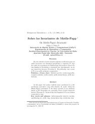
f<strong>in</strong>est level is reached aga<strong>in</strong>. Figure 2 illustrates this approach. Regulariz<strong>in</strong>g a<br />
256 2 <strong>image</strong> on a 700 MHz PC with 5 time steps per level requires about 0.3 CPU<br />
seconds.<br />
Figure 2. (a) Top: Restriction <strong>of</strong> a noisy test <strong>image</strong>. (b) Bottom: Regularizedby an AOS<br />
scheme embedded <strong>in</strong> a nested iteration strategy. From [35].<br />
4. Optic Flow Estimation<br />
Let us now <strong>in</strong>vestigate the use <strong>of</strong> <strong>nonl<strong>in</strong>ear</strong> <strong>diffusion</strong> processes <strong>in</strong> the context <strong>of</strong><br />
<strong>image</strong> sequence analysis. One <strong>of</strong> the ma<strong>in</strong> goals <strong>of</strong> <strong>image</strong> sequence analysis is<br />
the recovery <strong>of</strong> the so-called optic flow field. Optic flow describes the apparent<br />
motion <strong>of</strong> structures <strong>in</strong> the <strong>image</strong> plane. It can be used <strong>in</strong> a large variety <strong>of</strong>
44 J. WEICKERT<br />
applications rang<strong>in</strong>g from the recovery <strong>of</strong> motion parameters <strong>in</strong> robotics to the<br />
design <strong>of</strong> efficient algorithms for second generation video compression.<br />
In the follow<strong>in</strong>g we consider an <strong>image</strong> sequence f(x, y, z) where(x, y) ∈ Ω<br />
denotes the � location � <strong>and</strong> z ∈ [0,Z] is the time. We are look<strong>in</strong>g for the optic<br />
u(x,y,z)<br />
flow field<br />
which describes the correspondence <strong>of</strong> <strong>image</strong> structures at<br />
v(x,y,z)<br />
different times. Variational methods constitute one possibility to solve the optic<br />
flow problem; see e.g. [8, 14, 22, 37]. In [38] a method is considered which is<br />
based on the follow<strong>in</strong>g two assumptions:<br />
1. Image structures do not change their grey value over time. Therefore, along<br />
their path (x(z),y(z)) one obta<strong>in</strong>s<br />
(19)<br />
df (x(z),y(z),z)<br />
0 = = fxu + fyv + fz.<br />
dz<br />
2. As second assumption we impose a spatio-temporal smoothness constra<strong>in</strong>t:<br />
(20)<br />
�<br />
Ψ � |∇3u| 2 + |∇3v| 2� dx dy dz is “small”,<br />
Ω×[0,Z]<br />
where ∇3 := (∂x,∂y,∂z) T <strong>and</strong> Ψ is a regularizer as <strong>in</strong> the previous section.<br />
Comb<strong>in</strong><strong>in</strong>g these two constra<strong>in</strong>ts <strong>in</strong> a s<strong>in</strong>gle energy functional, one can obta<strong>in</strong> the<br />
optic flow as a m<strong>in</strong>imizer <strong>of</strong><br />
� �<br />
(21) Ef (u, v) := (fxu+fyv+fz) 2 + α Ψ � |∇3u| 2 + |∇3v| 2��<br />
dx dy dz.<br />
Ω×[0,Z]<br />
This functional can be regarded as a special representative <strong>of</strong> a much larger class<br />
<strong>of</strong> optic flow functionals for which one can establish general well-posedness results<br />
<strong>in</strong> H1 (Ω × (0,T)) × H1 (Ω × (0,T)). For more details the reader is referred to [37].<br />
The steepest descent equations for (21) with a differentiable regularizer Ψ are<br />
ut = ∇3· � Ψ ′ � |∇3u| 2 +|∇3v| 2� ∇3u � − 1<br />
α fx (22)<br />
(fxu+fyv+fz),<br />
vt = ∇3· � Ψ ′ � |∇3u| 2 +|∇3v| 2� ∇3v � − 1<br />
α fy (23)<br />
(fxu+fyv+fz).<br />
This is a coupled three-dimensional <strong>diffusion</strong>–reaction system. It may be treated<br />
numerically <strong>in</strong> the same way as the regularization methods from the last section.<br />
In matrix-vector notation, the result<strong>in</strong>g AOS scheme is given by<br />
(24)<br />
(25)<br />
u k+1 = 1<br />
3<br />
v k+1 = 1<br />
3<br />
3�<br />
l=1<br />
3�<br />
l=1<br />
�<br />
3τ I + α f 2 xI − 3τAl(uk ,vk ) �−1 � k τ u − αfx �<br />
fyvk ��<br />
+fz ,<br />
�<br />
3τ I + α f 2 y I − 3τAl(uk ,vk ) �−1 � k τ v − αfy �<br />
fxuk ��<br />
+fz .<br />
S<strong>in</strong>ce the cont<strong>in</strong>uous <strong>and</strong> discrete processes are globally convergent for convex<br />
diffusivities, the specific choice <strong>of</strong> the <strong>in</strong>itial values is not very important. In our<br />
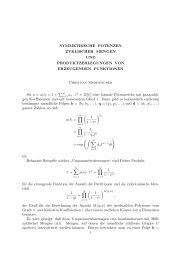
experiments the flow is <strong>in</strong>itialized with zero. Figure 3 shows an example. We
DIFFUSION IN COMPOTER VISION 45<br />
can see that the recovered optic flow field gives a quite realistic description <strong>of</strong> the<br />
person’s movement towards the camera.<br />
Figure 3. (a) Left: One frame <strong>of</strong> a hallway sequence with 256 × 256 × 16 pixels. A person is<br />
approach<strong>in</strong>g the camera. (b) Middle: Detail. (c) Right: Computedoptic flow. From [38] .<br />
5. Geodesic Active Contours<br />
5.1. Basic Idea <strong>and</strong> Theoretical Properties<br />
Active contours [18] play an important role <strong>in</strong> <strong>in</strong>teractive <strong>image</strong> segmentation, <strong>in</strong><br />
particular for medical applications. The basic idea is that the user specifies an<br />
<strong>in</strong>itial guess <strong>of</strong> an <strong>in</strong>terest<strong>in</strong>g contour (organ, tumour, . . . ). Then this contour is<br />
moved by <strong>image</strong>-driven forces to the edges <strong>of</strong> the desired object.<br />
So-called geodesic active contour models [4, 20] achieve this by apply<strong>in</strong>g a<br />
specific k<strong>in</strong>d <strong>of</strong> level set ideas [31]. In its simplest form, a geodesic active contour<br />
model consists <strong>of</strong> the follow<strong>in</strong>g steps. One embeds the user-specified <strong>in</strong>itial curve<br />
C0(s) as a zero level curve <strong>in</strong>to a function u0 : R2 → R, for <strong>in</strong>stance by us<strong>in</strong>g<br />
the distance transformation. Then u0 is evolved under a PDE which <strong>in</strong>cludes<br />
knowledge about the orig<strong>in</strong>al <strong>image</strong> f:<br />
�<br />
(26) ∂tu = |∇u| div g(|∇fσ| 2 ) ∇u<br />
�<br />
,<br />
|∇u|<br />
where g <strong>in</strong>hibits evolution at edges <strong>of</strong> f. One may choose decreas<strong>in</strong>g functions<br />
such as (6). Experiments <strong>in</strong>dicate that, <strong>in</strong> general, (26) will have nontrivial steady<br />
states. The evolution is stopped at some time T , when the process does hardly<br />
alter anymore, <strong>and</strong> the f<strong>in</strong>al contour C is extracted as the zero level curve <strong>of</strong><br />
u(x, T ). Figure 4 gives an example <strong>of</strong> such a geodesic active contour evolution.<br />
It can be <strong>in</strong>terpreted as a curve evolution that follows a modified mean curvature<br />
motion.
46 J. WEICKERT<br />
The theoretical analysis from [4, 20] shows that the <strong>in</strong>itial value problem has<br />
a unique viscosity solution u ∈ L ∞ (0,T; W 1,∞ (R 2 )) ∩ C([0, ∞) × R 2 ) for <strong>in</strong>itial<br />
data u0 ∈ C(R 2 ) ∩ W 1,∞ (R 2 ). This solution satisfies an extremum pr<strong>in</strong>ciple <strong>and</strong><br />
depends cont<strong>in</strong>uously on the <strong>in</strong>itial data with respect to the L ∞ norm.<br />
Figure 4. Temporal evolution <strong>of</strong> a geodesic active contour superimposed on the orig<strong>in</strong>al <strong>image</strong><br />
(Ω = (0, 256) 2 , λ =5,σ =1). From Left to Right: t = 0, 1500, 7500. Larger values for t do<br />
not alter the result .<br />
5.2. Numerical Approximation<br />
Next we present a novel scheme for the geodesic active contour model. Although<br />
(26) is not a <strong>diffusion</strong> process <strong>in</strong> a strict sense – it cannot be written <strong>in</strong> divergence<br />
form – one may use similar techniques as before.<br />
The case ∇u = 0 can be treated numerically by impos<strong>in</strong>g no changes at these<br />
po<strong>in</strong>ts. Several modifications are possible, but this case is less important s<strong>in</strong>ce one<br />
is <strong>in</strong>terested <strong>in</strong> steady states where the embedded level set does not vanish. Let<br />
us therefore consider the case where ∇u �= 0<strong>in</strong>somepixeli. Here straightforward<br />
f<strong>in</strong>ite difference implementations would give rise to problems when ∇u vanishes <strong>in</strong><br />
the 4-neighbourhood N (i) <strong>of</strong>i. These problems do not appear if one uses a f<strong>in</strong>ite<br />
difference scheme with harmonic averag<strong>in</strong>g. In its semi-implicit formulation such<br />
a scheme reads<br />
u<br />
(27)<br />
k+1<br />
i − uk i<br />
= |∇u|<br />
τ<br />
k � 2<br />
i<br />
( |∇u|<br />
u k+1<br />
j − uk+1 i<br />
h2 .<br />
j∈N (i)<br />
g ) k |∇u| +( j g ) k<br />
i<br />
Note that the denom<strong>in</strong>ator cannot vanish <strong>in</strong> this scheme. One can also verify that<br />
such a scheme is absolutely stable, s<strong>in</strong>ce it satisfies the discrete extremum pr<strong>in</strong>ciple<br />
(28) m<strong>in</strong><br />
i u0,i ≤ u k j ≤ max<br />
i u0,i<br />
for all j <strong>and</strong> for all k>0. An AOS variant <strong>of</strong> this scheme can be constructed <strong>in</strong><br />
exactly the same manner as <strong>in</strong> Section 2. The only difference is that Al(u k ) u k+1<br />
is now a semi-implicit discretization <strong>of</strong> |∇u|∂xl (g∇u/|∇u|) <strong>in</strong>stead <strong>of</strong> ∂xl (g∇u). It<br />
may be accelerated by embedd<strong>in</strong>g it <strong>in</strong> a multilevel framework as is described <strong>in</strong><br />
Section 3.2. The AOS scheme for geodesic active contours also <strong>in</strong>herits absolute
DIFFUSION IN COMPOTER VISION 47<br />
stability from (27), while a simple explicit variant <strong>of</strong> (27) would only be stable for<br />
τ ≤ h2 /8.<br />
It should be mentioned that this AOS strategy is not the only AOS approach<br />
that has been proposed for geodesic active contours. In [12], Goldenberg et al.<br />
present a method that requires to apply a distance transformation <strong>in</strong> each iteration<br />
[31]. This is done <strong>in</strong> order to obta<strong>in</strong> |∇u| = 1 such that (26) becomes the <strong>diffusion</strong><br />
process<br />
(29) ∂tu = div � g(|∇fσ| 2 ) ∇u �<br />
for which the st<strong>and</strong>ard AOS from Section 2 is used. S<strong>in</strong>ce our method does not<br />
require any time-consum<strong>in</strong>g distance transformation <strong>in</strong> each iteration step, it is<br />
simpler <strong>and</strong> computationally more efficient.<br />
5.3. Evaluation <strong>in</strong> Case <strong>of</strong> Mean Curvature Motion<br />
It is obvious that the preced<strong>in</strong>g AOS-based harmonic averag<strong>in</strong>g scheme can also be<br />
used for comput<strong>in</strong>g mean curvature motion for the case g = 1. In this situation a<br />
simple numerical evaluation is possible: S<strong>in</strong>ce it is well-known that a disk-shaped<br />
level set with area S(0) shr<strong>in</strong>ks under mean curvature motion such that<br />
(30) S(t) =S(0) − 2πt,<br />
simple accuracy evaluations are possible. To this end we used a distance transformation<br />
<strong>of</strong> some disk-shaped <strong>in</strong>itial <strong>image</strong> <strong>and</strong> considered the evolution <strong>of</strong> a level set<br />
with an <strong>in</strong>itial area <strong>of</strong> 24845 pixels. Table 2 shows the area errors for different time<br />
step sizes τ <strong>and</strong> two stopp<strong>in</strong>g times. We observe that for τ ≤ 5, the accuracy is<br />
sufficiently high for typical <strong>image</strong> process<strong>in</strong>g applications. Figure 5 demonstrates<br />
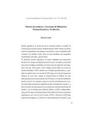
that <strong>in</strong> this case no violations regard<strong>in</strong>g rotational <strong>in</strong>variance are visible.<br />
Figure 5. Temporal evolution <strong>of</strong> a disked shaped level set under mean curvature motion. The<br />
results have been obta<strong>in</strong>edus<strong>in</strong>g an AOS-basedsemi-implicit scheme with harmonic averag<strong>in</strong>g<br />
<strong>and</strong>step size τ =5. From Left to Right: t = 0, 2250, 3600.
48 J. WEICKERT<br />
step size τ stopp<strong>in</strong>g time T = 2250 stopp<strong>in</strong>g time T = 3600<br />
0.5 −0.27 % −0.60 %<br />
1 −0.26 % −0.88 %<br />
2 −0.27 % −0.88 %<br />
5 −0.34 % −1.73 %<br />
10 −5.18 % 51.20 %<br />
Table 2. Area errors for the evolution <strong>of</strong> a disk-shaped area <strong>of</strong> 24845 pixels under mean curvature<br />
motion us<strong>in</strong>g an AOS-basedsemi-implicit scheme with harmonic averag<strong>in</strong>g. The pixels have<br />
size 1 <strong>in</strong> each direction.<br />
References<br />
1. Acton S. T., Multigrid anisotropic <strong>diffusion</strong>, IEEE Transactions on Image Process<strong>in</strong>g 7<br />
(1998), 280–291.<br />
2. Alvarez L., Lions P.-L. <strong>and</strong>Morel J.-M., Image selective smooth<strong>in</strong>g <strong>and</strong> edge detection by<br />
<strong>nonl<strong>in</strong>ear</strong> <strong>diffusion</strong>. II, SIAM Journal on Numerical Analysis 29 (1992), 845–866.<br />
3. Bänsch E. <strong>and</strong>Mikula K., A coarsen<strong>in</strong>g f<strong>in</strong>ite element strategy <strong>in</strong> <strong>image</strong> selective smooth<strong>in</strong>g,<br />
Computation <strong>and</strong>Visualization <strong>in</strong> Science 1 (1997), 53–61.<br />
4. Caselles V., Kimmel R. <strong>and</strong>Sapiro G., Geodesic active contours, International Journal <strong>of</strong><br />
Computer Vision 22 (1997), 61–79.<br />
5. Caselles V., Morel J.-M., Sapiro G. <strong>and</strong>Tannenbaum A., eds., Special Issue on Partial<br />
Differential Equations <strong>and</strong>Geometry-Driven Diffusion <strong>in</strong> Image Process<strong>in</strong>g <strong>and</strong>Analysis,<br />
Vol. 7(3) <strong>of</strong> IEEE Transactions on Image Process<strong>in</strong>g, IEEE Signal Process<strong>in</strong>g Society Press,<br />
Mar. 1998.<br />
6. Catté F., Lions P.-L., Morel J.-M. <strong>and</strong>Coll T., Image selective smooth<strong>in</strong>g <strong>and</strong> edge detection<br />
by <strong>nonl<strong>in</strong>ear</strong> <strong>diffusion</strong>, SIAM Journal on Numerical Analysis 32 (1992), 1895–1909.<br />
7. Charbonnier P., Blanc-FéraudL., Aubert G. <strong>and</strong>BarlaudM., Two determ<strong>in</strong>istic halfquadratic<br />
regularization algorithms for computed imag<strong>in</strong>g, In Proc. 1994 IEEE International<br />
Conference on Image Process<strong>in</strong>g, Vol. 2, Aust<strong>in</strong>, TX, IEEE Computer Society Press,<br />
pp. 168–172, Nov. 1994.<br />
8. Cohen I., Nonl<strong>in</strong>ear variational method for optical flow computation, In Proc. Eighth Sc<strong>and</strong><strong>in</strong>avian<br />
Conference on Image Analysis, Vol. 1, Tromsø, Norway, pp. 523–530, May 1993.<br />
9. Deriche R. <strong>and</strong>Faugeras O., Les EDP en traitement des <strong>image</strong>s et vision par ord<strong>in</strong>ateur,<br />
Traitement du Signal 13 (1996), pp. 551–577, Numéro Special.<br />
10. Fonta<strong>in</strong>e F. L. <strong>and</strong>Basu S., Wavelet-based solution to anisotropic <strong>diffusion</strong> equation for edge<br />
detection, International Journal <strong>of</strong> Imag<strong>in</strong>g Systems <strong>and</strong>Technology 9 (1998), 356–368.<br />
11. Fröhlich J. <strong>and</strong>Weickert J., Image process<strong>in</strong>g us<strong>in</strong>g a wavelet algorithm for <strong>nonl<strong>in</strong>ear</strong> <strong>diffusion</strong>,<br />
Tech. Rep. 104, Laboratory <strong>of</strong> Technomathematics, University <strong>of</strong> Kaiserslautern,<br />
Germany, Mar. 1994.<br />
12. Goldenberg R., Kimmel R., Rivl<strong>in</strong> E. <strong>and</strong> Rudzsky M., Fast geodesic active contours, <strong>in</strong><br />
Scale-Space Theories <strong>in</strong> Computer Vision (M. Nielsen, P. Johansen, O. F. Olsen <strong>and</strong>J. Weickert,<br />
eds.), Vol. 1682 <strong>of</strong> Lecture Notes <strong>in</strong> Computer Science, pp. 34–45, Spr<strong>in</strong>ger, Berl<strong>in</strong>,<br />
1999.<br />
13. H<strong>and</strong>lovičová A., Mikula K. <strong>and</strong>Sgallari F., Variational numerical methods for solv<strong>in</strong>g<br />
<strong>diffusion</strong> equation aris<strong>in</strong>g <strong>in</strong> <strong>image</strong> process<strong>in</strong>g, Journal <strong>of</strong> Visual Communication <strong>and</strong>Image<br />
Representation, (2001), to appear.<br />
14. Horn B. <strong>and</strong>Schunck B., Determ<strong>in</strong><strong>in</strong>g optical flow, Artificial Intelligence 17 (1981), 185–203.<br />
15. HummelR.A.,Representations based on zero-cross<strong>in</strong>gs <strong>in</strong> scale space, <strong>in</strong> Proc. 1986 IEEE<br />
Computer Society Conference on Computer Vision <strong>and</strong>Pattern Recognition, Miami Beach,<br />
FL, June 1986, IEEE Computer Society Press, pp. 204–209.
DIFFUSION IN COMPOTER VISION 49<br />
16. Ito K. <strong>and</strong>Kunisch K., An active set strategy based on the augmented Lagrangian formulation<br />
for <strong>image</strong> restoration, RAIRO Mathematical Models <strong>and</strong> Numerical Analysis 33 (1999),<br />
1–21.<br />
17. Jawerth B., L<strong>in</strong> P. <strong>and</strong>S<strong>in</strong>z<strong>in</strong>ger E., Lattice Boltzmann models for anisotropic <strong>diffusion</strong> <strong>of</strong><br />
<strong>image</strong>s, Journal <strong>of</strong> Mathematical Imag<strong>in</strong>g <strong>and</strong>Vision 11 (1999), 231–237.<br />
18. Kass M., Witk<strong>in</strong> A. <strong>and</strong>Terzopoulos D., Snakes: Active contour models, International<br />
Journal <strong>of</strong> Computer Vision 1 (1988), 321–331.<br />
19. Kačur J. <strong>and</strong>Mikula K., Solution <strong>of</strong> <strong>nonl<strong>in</strong>ear</strong> <strong>diffusion</strong> appear<strong>in</strong>g <strong>in</strong> <strong>image</strong> smooth<strong>in</strong>g <strong>and</strong><br />
edge detection, AppliedNumerical Mathematics 17 (1995), 47–59.<br />
20. Kichenassamy S., Kumar A., Olver P., Tannenbaum A. <strong>and</strong>Yezzi A., Conformal curvature<br />
flows: from phase transitions to active vision, Archive for Rational Mechanics <strong>and</strong>Analysis<br />
134 (1996), 275–301.<br />
21. Marchuk G. I., Splitt<strong>in</strong>g <strong>and</strong> alternat<strong>in</strong>g direction methods, <strong>in</strong> H<strong>and</strong>book <strong>of</strong> Numerical Analysis<br />
(P. G. Ciarlet <strong>and</strong>J.-L. Lions, eds.), Vol. I, pp. 197–462, North Holl<strong>and</strong>, Amsterdam,<br />
1990.<br />
22. Nagel H.-H. <strong>and</strong>Enkelmann W., An <strong>in</strong>vestigation <strong>of</strong> smoothness constra<strong>in</strong>ts for the estimation<br />
<strong>of</strong> displacement vector fields from <strong>image</strong> sequences, IEEE Transactions on Pattern<br />
Analysis <strong>and</strong>Mach<strong>in</strong>e Intelligence 8 (1986), 565–593.<br />
23. Nielsen M., Johansen P., Olsen O. F. <strong>and</strong>Weickert J., eds., Scale-Space Theories <strong>in</strong> Computer<br />
Vision, Vol.1682 <strong>of</strong> Lecture Notes <strong>in</strong> Computer Science, Spr<strong>in</strong>ger, Berl<strong>in</strong>, 1999.<br />
24. Niessen W. J., V<strong>in</strong>cken K. L., Weickert J. <strong>and</strong>Viergever M. A., Nonl<strong>in</strong>ear multiscale representations<br />
for <strong>image</strong> segmentation, Computer Vision <strong>and</strong> Image Underst<strong>and</strong><strong>in</strong>g 66 (1997),<br />
233–245.<br />
25. Nordström N., Biased anisotropic <strong>diffusion</strong> – a unified regularization <strong>and</strong> <strong>diffusion</strong> approach<br />
to edge detection, Image <strong>and</strong>Vision Comput<strong>in</strong>g 8 (1990), 318–327.<br />
26. Perona P. <strong>and</strong>Malik J., Scale space <strong>and</strong> edge detection us<strong>in</strong>g anisotropic <strong>diffusion</strong>, IEEE<br />
Transactions on Pattern Analysis <strong>and</strong>Mach<strong>in</strong>e Intelligence 12 (1990), 629–639.<br />
27. Preußer T. <strong>and</strong>Rumpf M., An adaptive f<strong>in</strong>ite element method for large scale <strong>image</strong> process<strong>in</strong>g,<br />
<strong>in</strong> Scale-Space Theories <strong>in</strong> Computer Vision (M. Nielsen, P. Johansen, O. F. Olsen, <strong>and</strong><br />
J. Weickert, eds.), Vol. 1682 <strong>of</strong> Lecture Notes <strong>in</strong> Computer Science, pp. 223–234, Spr<strong>in</strong>ger,<br />
Berl<strong>in</strong>, 1999.<br />
28. Ranjan U. S. <strong>and</strong>Ramakrishnan K. R., A stochastic scale space for multiscale <strong>image</strong> representation,<br />
<strong>in</strong> Scale-Space Theories <strong>in</strong> Computer Vision (M. Nielsen, P. Johansen, O. F.<br />
Olsen, <strong>and</strong>J. Weickert, eds.), Vol. 1682 <strong>of</strong> Lecture Notes <strong>in</strong> Computer Science, pp. 441–446,<br />
Spr<strong>in</strong>ger, Berl<strong>in</strong>, 1999.<br />
29. Scherzer O. <strong>and</strong>Weickert J., Relations between regularization <strong>and</strong> <strong>diffusion</strong> filter<strong>in</strong>g, Journal<br />
<strong>of</strong> Mathematical Imag<strong>in</strong>g <strong>and</strong>Vision 12 (2000), 43–63.<br />
30. Schnörr C., Unique reconstruction <strong>of</strong> piecewise smooth <strong>image</strong>s by m<strong>in</strong>imiz<strong>in</strong>g strictly convex<br />
non-quadratic functionals, Journal <strong>of</strong> Mathematical Imag<strong>in</strong>g <strong>and</strong>Vision 4 (1994), 189–198.<br />
31. Sethian J. A., Level Set Methods <strong>and</strong> Fast March<strong>in</strong>g Methods, Cambridge University Press,<br />
Cambridge, UK, 1999.<br />
32. ter Haar Romeny B., Florack L. <strong>and</strong> Koender<strong>in</strong>k J., eds., Scale-Space Theory <strong>in</strong> Computer<br />
Vision, Vol.1252 <strong>of</strong> Lecture Notes <strong>in</strong> Computer Science, Spr<strong>in</strong>ger, Berl<strong>in</strong>, 1997.<br />
33. terHaarRomenyB.M.,ed.,Geometry-Driven Diffusion <strong>in</strong> Computer Vision, Vol.1 <strong>of</strong><br />
Computational Imag<strong>in</strong>g <strong>and</strong>Vision, Kluwer, Dordrecht, 1994.<br />
34. Weickert J., Anisotropic Diffusion <strong>in</strong> Image Process<strong>in</strong>g, Teubner, Stuttgart, 1998.<br />
35. , Efficient <strong>image</strong> segmentation us<strong>in</strong>g partial differential equations <strong>and</strong> morphology,<br />
Pattern Recognition 34 (2001), 1813–1824.<br />
36. Weickert J., Heers J., Schnörr C., Zuiderveld K. J., Scherzer O. <strong>and</strong> Stiehl H. S., Fast<br />
parallel algorithms for a broad class <strong>of</strong> <strong>nonl<strong>in</strong>ear</strong> variational <strong>diffusion</strong> approaches, Real-<br />
Time Imag<strong>in</strong>g 7 (2001), 31–45.
50 J. WEICKERT<br />
37. Weickert J. <strong>and</strong>Schnörr C., A theoretical framework for convex regularizers <strong>in</strong> PDE-based<br />
computation <strong>of</strong> <strong>image</strong> motion, Tech. Rep. 13/2000, Computer Science Series, University <strong>of</strong><br />
Mannheim, Germany, June 2000, to appear <strong>in</strong> International Journal <strong>of</strong> Computer Vision.<br />
38. , Variational optic flow computation with a spatio-temporal smoothness constra<strong>in</strong>t,<br />
Journal <strong>of</strong> Mathematical Imag<strong>in</strong>g <strong>and</strong>Vision 14 (2001), 245–255.<br />
39. Weickert J., ter Haar Romeny B. M. <strong>and</strong>Viergever M. A., Efficient <strong>and</strong> reliable schemes<br />
for <strong>nonl<strong>in</strong>ear</strong> <strong>diffusion</strong> filter<strong>in</strong>g, IEEE Transactions on Image Process<strong>in</strong>g 7 (1998), 398–410.<br />
J. Weickert, Computer Vision, Graphics, <strong>and</strong>Pattern Recognition Group, Department <strong>of</strong> Mathematics<br />
<strong>and</strong>Computer Science, University <strong>of</strong> Mannheim, 68131 Mannheim, Germany, e-mail:<br />
Joachim.Weickert@uni-mannheim.de,<br />
http://www.cvgpr.uni-mannheim.de/weickert