Parallel Coordinate Descent for L1-Regularized Loss Minimization

More documents

Recommendations

Info

Parallel Coordinate Descent for L 1-Regularized Loss Minimization maximum P as P ∗ ≡ ceiling( d ρ ). For an ideal problem with uncorrelated features, ρ = 1, so we could do up to P ∗ = d parallel updates. For a pathological problem with exactly correlated features, ρ = d, so our theorem tells us that we could not do parallel updates. With P = 1, we recover the result for Shooting in Theorem 2.1. To prove Theorem 3.2, we first bound the negative impact of interference between parallel updates. Lemma 3.3. Fix x. Under the assumptions and definitions from Theorem 3.2, if ∆x is the collective update to x in one iteration of Alg. 2, then E Pt [F (x + ∆x) − F (x)] ≤ PE j [δx j (∇F (x)) j + β 2 ( 1 − (P−1)ρ 2d ) ] (δx j ) 2 , where E Pt is w.r.t. a random choice of P t and E j is w.r.t. choosing j ∈ {1, . . . , 2d} uniformly at random. Proof Sketch: Take the expectation w.r.t. P t of the inequality in Assumption 3.1. E Pt [F (x + ∆x) − F (x)] ≤ E Pt [ ∆x T ∇F (x) + β 2 ∆xT A T A∆x ] (8) Separate the diagonal elements from the second order term, and rewrite the expectation using our independent choices of i j ∈ P t . (Here, δx j is the update given by (5), regardless of whether j ∈ P t .) = PE j [ δxj(∇F (x)) j + β 2 (δxj)2] + β 2 P(P − 1)Ei [ Ej [ δxi(A T A) i,jδx j ]] (9) Upper bound the double expectation in terms of E j [ (δxj ) 2] by expressing the spectral radius ρ of A T A as ρ = max z: z T z=1 z T (A T A)z. E i [ E j [ δx i(A T A) i,jδx j ]] ≤ ρ 2d Ej [ (δxj) 2] (10) Combine (10) back into (9), and rearrange terms to get the lemma’s result. Proof Sketch (Theorem 3.2): Our proof resembles Shalev-Shwartz and Tewari (2009)’s proof of Theorem 2.1. The result from Lemma 3.3 replaces Assumption 2.1. One bound requires (P−1)ρ 2d < 1. Our analysis implicitly assumes that parallel updates of the same weight x j will not make x j negative. Proper write-conflict resolution can ensure this assumption holds and is viable in our multicore setting. 3.2. Theory vs. Empirical Performance We end this section by comparing the predictions of Theorem 3.2 about the number of parallel updates P with empirical performance for Lasso. We exactly 10 4.5 T (iterations)104.7 P (parallel updates) 10 4.3 10 0 P*=3 T (iterations) P*=158 10 2 10 0 10 1 (parallel 10 2 updates) 10 3 Data: Ball64 singlepixcam Data: Mug32 singlepixcam d = 4096, ρ = 2047.8 d = 1024, ρ = 6.4967 Figure 2. Theory for Shotgun’s P (Theorem 3.2) vs. empirical performance for Lasso on two datasets. Y-axis has iterations T until E Pt [F (x (T ) )] came within 0.5% of F (x ∗ ). Thick red lines trace T for increasing P (until too large P caused divergence). Vertical lines mark P ∗ . Dotted diagonal lines show optimal (linear) speedups (partly hidden by solid line in right-hand plot). simulated Shotgun as in Alg. 2 to eliminate effects from the practical implementation choices made in Sec. 4. We tested two single-pixel camera datasets from Duarte [ et al. (2008) with very different ρ, estimating E Pt F (x (T ) ) ] by averaging 10 runs of Shotgun. We used λ = 0.5 for Ball64 singlepixcam to get x ∗ with about 27% non-zeros; we used λ = 0.05 for Mug32 singlepixcam to get about 20% non-zeros. Fig. [ 2 plots P versus the iterations T required for E Pt F (x (T ) ) ] to come within 0.5% of the optimum F (x ∗ ). Theorem 3.2 predicts that T should decrease as 1 P as long as P < P∗ ≈ d ρ +1. The empirical behavior follows this theory: using the predicted P ∗ gives almost optimal speedups, and speedups are almost linear in P. As P exceeds P ∗ , Shotgun soon diverges. Fig. 2 confirms Theorem 3.2’s result: Shooting, a seemingly sequential algorithm, can be parallelized and achieve near-linear speedups, and the spectral radius of A T A succinctly captures the potential for parallelism in a problem. To our knowledge, our convergence results are the first for parallel coordinate descent for L 1 -regularized losses, and they apply to any convex loss satisfying Assumption 3.1. Though Fig. 2 ignores certain implementation issues, we show in the next section that Shotgun performs well in practice. 3.3. Beyond L 1 Theorems 2.1 and 3.2 generalize beyond L 1 , for their main requirements (Assumptions 2.1, 3.1) apply to a more general class of problems: min F (x) s.t. x ≥ 0, where F (x) is smooth. We discuss Shooting and Shotgun for sparse regression since both the method (coordinate descent) and problem (sparse regression) are arguably most useful for high-dimensional settings.
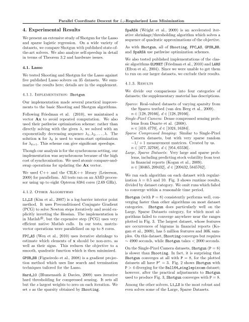
Parallel Coordinate Descent for L 1-Regularized Loss Minimization 4. Experimental Results We present an extensive study of Shotgun for the Lasso and sparse logistic regression. On a wide variety of datasets, we compare Shotgun with published state-ofthe-art solvers. We also analyze self-speedup in detail in terms of Theorem 3.2 and hardware issues. 4.1. Lasso We tested Shooting and Shotgun for the Lasso against five published Lasso solvers on 35 datasets. We summarize the results here; details are in the supplement. 4.1.1. Implementation: Shotgun Our implementation made several practical improvements to the basic Shooting and Shotgun algorithms. Following Friedman et al. (2010), we maintained a vector Ax to avoid repeated computation. We also used their pathwise optimization scheme: rather than directly solving with the given λ, we solved with an exponentially decreasing sequence λ 1 , λ 2 , . . . , λ. The solution x for λ k is used to warm-start optimization for λ k+1 . This scheme can give significant speedups. Though our analysis is for the synchronous setting, our implementation was asynchronous because of the high cost of synchronization. We used atomic compare-andswap operations for updating the Ax vector. We used C++ and the CILK++ library (Leiserson, 2009) for parallelism. All tests ran on an AMD processor using up to eight Opteron 8384 cores (2.69 GHz). 4.1.2. Other Algorithms L1 LS (Kim et al., 2007) is a log-barrier interior point method. It uses Preconditioned Conjugate Gradient (PCG) to solve Newton steps iteratively and avoid explicitly inverting the Hessian. The implementation is in Matlab R○ , but the expensive step (PCG) uses very efficient native Matlab calls. In our tests, matrixvector operations were parallelized on up to 8 cores. FPC AS (Wen et al., 2010) uses iterative shrinkage to estimate which elements of x should be non-zero, as well as their signs. This reduces the objective to a smooth, quadratic function which is then minimized. GPSR BB (Figueiredo et al., 2008) is a gradient projection method which uses line search and termination techniques tailored for the Lasso. Hard l0 (Blumensath & Davies, 2009) uses iterative hard thresholding for compressed sensing. It sets all but the s largest weights to zero on each iteration. We set s as the sparsity obtained by Shooting. SpaRSA (Wright et al., 2009) is an accelerated iterative shrinkage/thresholding algorithm which solves a sequence of quadratic approximations of the objective. As with Shotgun, all of Shooting, FPC AS, GPSR BB, and SpaRSA use pathwise optimization schemes. We also tested published implementations of the classic algorithms GLMNET (Friedman et al., 2010) and LARS (Efron et al., 2004). Since we were unable to get them to run on our larger datasets, we exclude their results. 4.1.3. Results We divide our comparisons into four categories of datasets; the supplementary material has descriptions. Sparco: Real-valued datasets of varying sparsity from the Sparco testbed (van den Berg et al., 2009). n ∈ [128, 29166], d ∈ [128, 29166]. Single-Pixel Camera: Dense compressed sensing problems from Duarte et al. (2008). n ∈ [410, 4770], d ∈ [1024, 16384]. Sparse Compressed Imaging: Similar to Single-Pixel Camera datasets, but with very sparse random −1/ + 1 measurement matrices. Created by us. n ∈ [477, 32768], d ∈ [954, 65536]. Large, Sparse Datasets: Very large and sparse problems, including predicting stock volatility from text in financial reports (Kogan et al., 2009). n ∈ [30465, 209432], d ∈ [209432, 5845762]. We ran each algorithm on each dataset with regularization λ = 0.5 and 10. Fig. 3 shows runtime results, divided by dataset category. We omit runs which failed to converge within a reasonable time period. Shotgun (with P = 8) consistently performs well, converging faster than other algorithms on most dataset categories. Shotgun does particularly well on the Large, Sparse Datasets category, for which most algorithms failed to converge anywhere near the ranges plotted in Fig. 3. The largest dataset, whose features are occurrences of bigrams in financial reports (Kogan et al., 2009), has 5 million features and 30K samples. On this dataset, Shooting converges but requires ∼ 4900 seconds, while Shotgun takes < 2000 seconds. On the Single-Pixel Camera datasets, Shotgun (P = 8) is slower than Shooting. In fact, it is surprising that Shotgun converges at all with P = 8, for the plotted datasets all have P ∗ = 3. Fig. 2 shows Shotgun with P > 4 diverging for the Ball64 singlepixcam dataset; however, after the practical adjustments to Shotgun used to produce Fig. 3, Shotgun converges with P = 8. Among the other solvers, L1 LS is the most robust and even solves some of the Large, Sparse Datasets.
Page 1 and 2: Parallel Coordinate Descent for L 1
Page 3: Parallel Coordinate Descent for L 1
Page 7 and 8: Parallel Coordinate Descent for L 1

Parallel Coordinate Descent for L1-Regularized Loss Minimization

Create successful ePaper yourself

Delete template?

Save as template?