Parallel Coordinate Descent for L1-Regularized Loss Minimization

More documents

Recommendations

Info

Parallel Coordinate Descent for L 1-Regularized Loss Minimization Other alg. runtime (sec) 100 Shotgun faster 10 Other alg. runtime (sec) 40 Shotgun faster 10 Shotgun slower Other alg. runtime (sec) 44 Shotgun faster 10 Shotgun slower 1000 100 10 10 100 1000 8000 Shotgun runtime (sec) Other alg. runtime (sec)8000 Shotgun faster Shotgun slower 1 Shotgun slower 1 2 1 2 Shooting 1 10 100 1 10 40 1 10 44 Shotgun runtime (sec) 2 Shotgun runtime (sec) Shotgun runtime L1_LS (sec) Shooting 1.8 (a) Sparco 2 Shooting FPC_AS L1_LS (b) Single-Pixel Camera (c) Sparse Compressed Img. 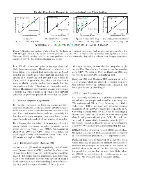(d) Large, Sparse Datasets P ∗ ∈ [3, 17366], avg 2987 P ∗ Shooting 1.8 2 = 3 P ∗ L1_LS GPSR_BB FPC_AS 1.8 ∈ [2865, 11779], avg 7688 P ∗ ∈ [214, 2072], avg 1143 2 Shooting 1.6 L1_LS FPC_AS SpaRSA GPSR_BB 1.8 Shooting L1_LS FPC_AS 1.6 GPSR_BB Hard_l0 SpaRSA 1.8 L1_LS 1.6 FPC_AS GPSR_BB SpaRSA Hard_l0 1.8 1.6 FPC_AS 1.4 Figure 3. Runtime comparison of algorithms GPSR_BB for theSpaRSA Lasso Hard_l0 1.6 GPSR_BB 1.4 on 4 dataset categories. Each marker compares an algorithm with Shotgun (with P = 8) on SpaRSA Hard_l0 1.4 one dataset (and one λ ∈ {0.5, 10}). Y-axis is that algorithm’s running time; X-axis is 1.6 SpaRSA Shotgun’s (P=8) running time on the same Hard_l0 problem. 1.2 Markers above the diagonal line indicate that Shotgun was faster; 1.4 Hard_l0 markers 1.2 1.4 below the line indicate Shotgun was slower. 1.4 1.2 1 1.2 1 1.2 1 1.4 1.6 1.8 2 It is 1.2 difficult to compare optimization 1 1.2 1.4 1.6 1.8 2 1.2 1 algorithms and Although our analysis uses the fixed step size in (5), their implementations. 1 1.2 1.4 1.6 1.8 2 1 Algorithms’ termination criteria differ; 1 e.g., primal-dual 1 1.2 methods 1.4 such 1.6 as L1 1.8 LS 2as in CDN. We refer to CDN as Shooting CDN, and we modified Shooting and Shotgun to use line searches 1 monitor1 the duality 1.2 gap, 1.4 while 1.6Shotgun 1.8 monitors 2 the we refer to parallel CDN as Shotgun CDN. 1 1.2 1.4 1.6 1.8 2 change in x. Shooting and Shotgun were written in C++, which is generally fast; the other algorithms were in Matlab, which handles loops slowly but linear algebra quickly. Therefore, we emphasize major trends: Shotgun robustly handles a range of problems; Theorem 3.2 helps explain its speedups; and Shotgun generally outperforms published solvers for the Lasso. 4.2. Sparse Logistic Regression For logistic regression, we focus on comparing Shotgun with Stochastic Gradient Descent (SGD) variants. SGD methods are of particular interest to us since they are often considered to be very efficient, especially for learning with many samples; they often have convergence bounds independent of the number of samples. For a large-scale comparison of various algorithms for sparse logistic regression, we refer the reader to the recent survey by Yuan et al. (2010). On L1 logreg (Koh et al., 2007) and CDN (Yuan et al., 2010), our results qualitatively matched their survey. Yuan et al. (2010) do not explore SGD empirically. 4.2.1. Implementation: Shotgun CDN As Yuan et al. (2010) show empirically, their Coordinate Descent Newton (CDN) method is often orders of magnitude faster than the basic Shooting algorithm (Alg. 1) for sparse logistic regression. Like Shooting, CDN does coordinate descent, but instead of using a fixed step size, it uses a backtracking line search starting at a quadratic approximation of the objective. Shooting CDN and Shotgun CDN maintain an active set of weights which are allowed to become non-zero; this scheme speeds up optimization, though it can limit parallelism by shrinking d. 4.2.2. Other Algorithms SGD iteratively updates x in a gradient direction estimated with one sample and scaled by a learning rate. We implemented SGD in C++ following, e.g., Zinkevich et al. (2010). We used lazy shrinkage updates (Langford et al., 2009a) to make use of sparsity in A. Choosing learning rates for SGD can be challenging. In our tests, constant rates led to faster convergence than decaying rates (decaying as 1/ √ T ). For each test, we tried 14 exponentially increasing rates in [10 −4 , 1] (in parallel) and chose the rate giving the best training objective. We did not use a sparsifying step for SGD. SMIDAS (Shalev-Shwartz & Tewari, 2009) uses stochastic mirror descent but truncates gradients to sparsify x. We tested their published C++ implementation. Parallel SGD refers to Zinkevich et al. (2010)’s work, which runs SGD in parallel on different subsamples of the data and averages the solutions x. We tested this method since it is one of the few existing methods for parallel regression, but we note that Zinkevich et al. (2010) did not address L 1 regularization in their analysis. We averaged over 8 instances of SGD.
Parallel Coordinate Descent for L 1-Regularized Loss Minimization 4.2.3. Results Fig. 4 plots training objectives and test accuracy (on a held-out 10% of the data) for two large datasets. The zeta dataset 5 illustrates the regime with n ≫ d. It contains 500K samples with 2000 features and is fully dense (in A). SGD performs well and is fairly competitive with Shotgun CDN (with P = 8). The rcv1 dataset 6 (Lewis et al., 2004) illustrates the high-dimensional regime (d > n). It has about twice as many features (44504) as samples (18217), with 17% non-zeros in A. Shotgun CDN (P = 8) was much faster than SGD, especially in terms of the objective. Parallel SGD performed almost identically to SGD. Though convergence bounds for SMIDAS are comparable to those for SGD, SMIDAS iterations take much longer due to the mirror descent updates. To execute 10M updates on the zeta dataset, SGD took 728 seconds, while SMIDAS took over 8500 seconds. These results highlight how SGD is orthogonal to Shotgun: SGD can cope with large n, and Shotgun can cope with large d. A hybrid algorithm might be scalable in both n and d and, perhaps, be parallelized over both samples and features. 4.3. Self-Speedup of Shotgun To study the self-speedup of Shotgun Lasso and Shotgun CDN, we ran both solvers on our datasets with varying λ, using varying P (number of parallel updates = number of cores). We recorded the running time as the first time when an algorithm came within 0.5% of the optimal objective, as computed by Shooting. Fig. 5 shows results for both speedup (in time) and speedup in iterations until convergence. The speedups in iterations match Theorem 3.2 quite closely. However, relative speedups in iterations (about 8×) are not matched by speedups in runtime (about 2× to 4×). We thus discovered that speedups in time were limited by low-level technical issues. To understand the limiting factors, we analyzed various Shotgun-like algorithms to find bottlenecks. 7 We found we were hitting the memory wall (Wulf & McKee, 1995); memory bus bandwidth and latency proved to be the most limiting factors. Each weight update requires an atomic update to the shared Ax vector, and the ratio of memory accesses to floating point operations is only O(1). Data 5 The zeta dataset is from the Pascal Large Scale Learning Challenge: http://www.mlbench.org/instructions/ 6 Our version of the rcv1 dataset is from the LIBSVM repository (Chang & Lin, 2001). 7 See the supplement for the scalability analysis details. Objective value Error (held−out data) 10 5.4 Shooting CDN 10 5.3 SGD Parallel SGD Shotgun CDN 10 5.2 0 500 1000 Time (sec) 0.15 0.1 Shooting CDN SGD Parallel SGD Shotgun CDN 500 1000 Time (sec) Objective value Error (held−out data) 8000 7000 6000 0.05 0.045 Shooting CDN Shotgun CDN SGD 10 Time (log scale, secs) Shooting CDN SGD Shotgun CDN 0.04 10 Time (log scale, secs) zeta with λ = 1 rcv1 with λ = 1 d = 2000, n = 500, 000 d = 44504, n = 18217 Figure 4. Sparse logistic regression on 2 datasets. Top plots trace training objectives over time; bottom plots trace classification error rates on held-out data (10%). On zeta (n ≫ d), SGD converges faster initially, but Shotgun CDN (P=8) overtakes it. On rcv1 (d > n), Shotgun CDN converges much faster than SGD (note the log scale); Parallel SGD (P=8) is hidden by SGD. accesses have no temporal locality since each weight update uses a different column of A. We further validated these conclusions by monitoring CPU counters. 5. Discussion We introduced the Shotgun, a simple parallel algorithm for L 1 -regularized optimization. Our convergence results for Shotgun are the first such results for parallel coordinate descent with L 1 regularization. Our bounds predict linear speedups, up to an interpretable, problem-dependent limit. In experiments, these predictions matched empirical behavior. Extensive comparisons showed that Shotgun outperforms state-of-the-art L 1 solvers on many datasets. We believe that, currently, Shotgun is one of the most efficient and scalable solvers for L 1 -regularized problems. The most exciting extension to this work might be the hybrid of SGD and Shotgun discussed in Sec. 4.3. Code, Data, and Benchmark Results: Available at http://www.select.cs.cmu.edu/projects Acknowledgments Thanks to John Langford, Guy Blelloch, Joseph Gonzalez, Yucheng Low and our reviewers for feedback. Funded by NSF IIS-0803333, NSF CNS-0721591, ARO MURI W911NF0710287, ARO MURI W911NF0810242.
Page 1 and 2: Parallel Coordinate Descent for L 1
Page 3 and 4: Parallel Coordinate Descent for L 1
Page 5: Parallel Coordinate Descent for L 1

Parallel Coordinate Descent for L1-Regularized Loss Minimization

Create successful ePaper yourself

Delete template?

Save as template?