Asteroid Occultations

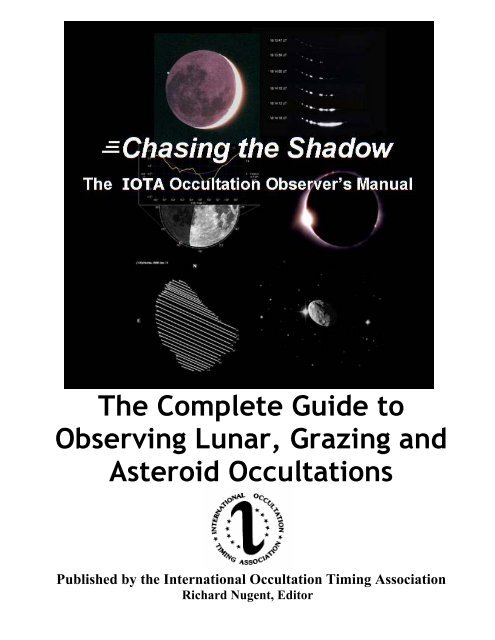
The Complete Guide to
Observing Lunar, Grazing and
Asteroid Occultations
Published by the International Occultation Timing Association
Richard Nugent, Editor

Copyright © 2007 International Occultation Timing Association, Richard Nugent, Editor. All rights reserved.
This publication may be reproduced, or copied in any manner freely for one’s own personal use, but it may
not be distributed or sold for money or for any other compensation.
This publication is protected under the 1976 United States Copyright Act. For any other use of the
publication, please contact the Editor and Publisher via email: RNugent@wt.net.
While the Editor, Authors and Publisher have made their best efforts in preparing the IOTA Occultation
Manual, they make no representation or warranties with respect to the accuracy and completeness regard to its
contents. The Publisher, Editor and Authors specifically disclaim any implied warranties of merchantability or
fitness of the material presented herein for any purpose. The advice and strategies contained herein may not
be suitable for your situation and the reader and/or user assumes full responsibility for using and attempting
the methods and techniques presented. Neither the publisher nor the authors shall be liable for any loss of
profit or any damages, including but not limited to special, incidental, consequential, or other damages and
any loss or injury. Persons are advised that occultation observations involve substantial risk and are advised to
take the necessary precautions before attempting such observations.
Editor in Chief: Richard Nugent
Assistant Editor: Lydia Lousteaux
Contributors: Trudy E. Bell, Dr. David Dunham, Dr. Joan Dunham, Paul Maley, Guy Nason, Richard Nugent,
Walt “Rob” Robinson, Arvind Paranjype, Dr. Roger Venable, Dr. Wayne Warren, Jr., James W. Young.
The IOTA Occultation Observer’s Manual is available to download from:
http://www.poyntsource.com/IOTAmanual/index.htm
Downloading of this publication and making a hardcopy for one’s self is encouraged to promote the
observation of occultation phenomenon.
The IOTA Manual is published by the International Occultation Timing Association
ISBN 978-0-615-29124-6
Cover Images:
Total occultation of star about to occur by
crescent Moon’s dark side near position
angle 65°
Lunar limb profile – Watts angle 164°
Baily’s Beads during total Solar Eclipse of
February 26, 1998. Mosaic of 6 video frames
covering a 33 second time interval
Diamond ring effect during total Solar Eclipse
Asteroid profile of 135 Hertha from occultation
Dec 11, 2008. Scotty Degenhardt obtained 14
of the 23 chords with his remote video stations
Asteroid about to pass in front of a star
1

Preface
An occultation (pronounced “Occ-kull-tay-shun”) occurs when the Moon, asteroid or other planetary
body eclipses a star momentarily blocking its light. Occultation observations have been used for
hundreds of years by sailors to determine time and their position at sea. Modern occultation
observations are routinely used to refine the orbit of the Moon, analyze the positions of stars and
the coordinate system they represent, detect new stellar companions, pinpoint the position of X-ray
and radio sources, determine the size and shape of lunar mountains, determine stellar diameters,
and the recent hot area of determining the size and shape of asteroids in our solar system. In 1985,
Pluto’s atmosphere was discovered by the occultation technique. In March 1977, the occultation of
a bright star by the planet Uranus resulted in the discovery of its ring system. This ring system
might actually have been seen indirectly by the discoverer of Uranus, William Herschel, as he
noticed faint stars dim as the planet passed close by.
Occultation observations are fun to observe. There is perhaps nothing more exciting than watching
a star vanish and return from behind a lunar mountain, or to see the star disappear for several
seconds as an asteroid passes in front of it. Anyone with a small telescope, tape recorder or
camcorder and shortwave radio can make valuable scientific observations to help determine the
size and shape of asteroids and to aid in new discoveries about these mysterious objects, including
some of the elusive small moons that orbit them.
This observer’s manual is the first comprehensive book of its kind to assist beginning observers get
started in occultation observations. This manual also shows advanced observers the latest in video
and GPS time insertion techniques. It is a How To guide in observing total and grazing occultations
of the moon, asteroid occultations and solar eclipses. Whether you are an observer with a small
telescope or an experienced observer with a video system, this book will show you how to set up
your equipment, predict, observe, record, report and analyze occultation observations whether you
are at a fixed site or have mobile capabilities.
The International Occultation Timing Association (IOTA) and its worldwide sister organizations
(Europe, United Kingdom, Australia/New Zealand, Japan, S. Asia/India, Mexico, Latin America,
South Africa) are here to assist you. We have online Internet discussion groups and observers are
in contact with each other nearly every day planning for the next occultation expedition or sharing
ideas on new equipment, software and new techniques. IOTA and several of its members have web
pages loaded with occultation information and methods, tips, software, predictions and results of
observations. The Internet has simplified occultation observations with predictions and results now
online. Equipment advances (especially video) along with accurate star and asteroid positions have
resulted in an explosion of occultation observations in the past ten years. Whereas between 1978
and 1998 less than 20 successful asteroid occultationswere observed each year, now there are over
150-200 successful asteroid events observed worldwide annually by numerous teams of observers.
The novice occultation observer will find the basics of occultations including how to observe and to
record them accurately using simple, inexpensive equipment. Advanced observers will find video
methods of recording occultations. This includes the use of the GPS satellites along with video time
inserters that can allow frame by frame analysis of observations providing timings accurate to a few
hundredths of a second !
2

The latest method for obtaining multiple chords on asteroid events comes from remote unattended
video stations. See Chapter 10, and Scotty Degenhardt’s 14 remote video stations used to
determine the size and shape of the asteroid 135 Hertha on page 139.
The potential for new discoveries continues with every new occultation observation. Astronomers,
both professional and amateur, are encouraged to get involved in this exciting field and on several
online occultation discussion groups to see what events are to occur in their area. Information on
how to get involved with IOTA and contact information is given in Appendix A, along with the many
IOTA organizations worldwide.
Please join us.
Acknowledgments
Richard Nugent
Editor, IOTA Occultation Observer’s Manual
Executive Secretary
International Occultation Timing Association
A project on occultations such as this is the product of decades of effort and work by the hundreds
of worldwide occultation observers, expedition leaders, software originators, and many others.
Without the dedicated efforts of these individuals, the modern occultation program would simply
not exist. Dr. David Dunham is the founder and only President of IOTA/USA, leading the way in the
occultation program in North America for over 46 years. Many pioneers have carved out the
methods and techniques of occultation observing including: Hal Povenmire, Paul Maley, Dr. Wayne
Warren Jr., Robert Sandy, Richard Wilds, Tom Campbell, Dr. Tom van Flandern, Steve Preston,
Walter Morgan, Walt Robinson, Don Stockbauer (USA), David Herald (Australia) Edwin Goffin, Jean
Meeus, Hans Bode, Eberherd Riedel (Europe), Gordon Taylor (UK), Dr. Mitsuru Soma, Dr. Isao Sato
(Japan) and numerous others.
Special thanks are due to the contributors Dr. David Dunham, Dr. Joan Dunham, Paul Maley, Guy
Nason, Walt “Rob” Robinson, Arvind Paranjype, Dr. Roger Venable, Dr. Wayne Warren, Jr., James
W. Young and Trudy E. Bell who submitted material in their field of expertise included in the
chapters in this book. Thanks is due to all of these individuals and the thousands of observers who
for the past 50 years have traveled worldwide and braved the elements with numerous equipment
and other hardships to make solar eclipse and occultation observations. Lydia Lousteaux, assistant
editor, proofread the entire book and made numerous suggestions and changes including the
rewriting of whole paragraphs. As Editor in Chief and contributing author of the IOTA Occultation
Observer’s Manual, I take full responsibility for the layout, content and accuracy of the information
presented. Nevertheless, in a project of this size some errors may have gone undetected. Please
direct any errors or corrections to me at RNugent@wt.net. Good luck in your occultation observing!
Richard Nugent
Houston, Texas
3

Contributors:
Trudy E. Bell
Dr. David Dunham
Dr. Joan Dunham
Paul Maley
Guy Nason
Richard Nugent
Walt “Rob” Robinson
Arvind Paranjype
Dr. Roger Venable
Dr. Wayne Warren
James W. Young
4

Table of Contents
1 INTRODUCTION TO OCCULTATIONS..........................................................................................10
5
1.1 SCIENTIFIC USES OF OCCULTATIONS.......................................................................................................................12
1.2 THE INTERNATIONAL OCCULTATION TIMING ASSOCIATION, IOTA.......................................................................16
1.3 THE INTERNATIONAL LUNAR OCCULTATION CENTER (ILOC) 1923-2009 .............................................................17
1.4 OCCULTATION FIRSTS..............................................................................................................................................18
1.5 IOTA GOALS AND OBJECTIVES ...............................................................................................................................21
1.5.1 Double Stars ....................................................................................................................................................22
1.5.2 Satellites of Asteroids.......................................................................................................................................22
1.6 Relativistic Effects……………………….…………………………...…………………………………23
2 OBSERVING PREREQUISITES..............................................................................................................24
2.1 SKILLS......................................................................................................................................................................24
2.2 RESOURCES ..............................................................................................................................................................24
2.2.1 Expenses...........................................................................................................................................................25
2.3 PERSONAL CONSIDERATIONS AND BEHAVIOR.........................................................................................................25
2.4 WHAT IF SOMETHING GOES WRONG? .....................................................................................................................27
2.5 OBSERVING POST-REQUISITES .................................................................................................................................27
3 TYPES OF OCCULTATION PROJECTS ..........................................................................................28
3.1 TOTAL OCCULTATIONS............................................................................................................................................28
3.2 METHODOLOGY .......................................................................................................................................................29
3.2.1 Equipment ........................................................................................................................................................30
3.2.2 The Telescope ..................................................................................................................................................30
3.2.3 Short Wave Receivers ......................................................................................................................................33
3.2.4 Recorders..........................................................................................................................................................34
3.2.5 Equipment Check List ......................................................................................................................................34
3.3 HOW TO OBSERVE A TOTAL OCCULTATION ............................................................................................................35
3.4 REDUCING THE OBSERVATION (QUICK OVERVIEW).................................................................................................38
3.5 SENDING IN YOUR OBSERVATIONS (QUICK OVERVIEW)..........................................................................................39
3.6 DOUBLE STARS ........................................................................................................................................................40
3.7 SAFETY CONSIDERATIONS ......................................................................................................................................41
4 PREDICTIONS ...................................................................................................................................................43
4.1 LUNAR OCCULTATION WORKBENCH (LOW) ...........................................................................................................43
4.2 OCCULT .................................................................................................................................................................49
4.2.1 Sample Total occultation output generated by Occult (partial listing):............................................................50
4.2.2 Eclipses and Transits........................................................................................................................................53
4.2.3 Asteroid Event Predictions...............................................................................................................................56
4.2.4 Ephemerides and Mutual Events.....................................................................................................................60
4.2.5 Record and Reduce...........................................................................................................................................60
4.2.6 Baily’s Beads....................................................................................................................................................61
4.2.7 How to obtain Occult Software ........................................................................................................................61
4.2.8 How to Obtain Predictions Only ......................................................................................................................61
4.3 ROYAL ASTRONOMICAL SOCIETY OF CANADA OBSERVER’S HANDBOOK..............................................................61
4.4 STANDARD STATION PREDICTIONS – IOTA WEBSITE.............................................................................................63
4.4.1 Standard Station Predictions and Your Location .............................................................................................64
4.5 TRAINING AND SIMULATION....................................................................................................................................65
4.5.1 Simulation Software.........................................................................................................................................66
4.6 RESULTS AND REPORTING OBSERVATIONS .............................................................................................................66
4.6.1 IOTA Website Publications..............................................................................................................................66

4.6.2 Reporting Your Lunar Occultation Observations ............................................................................................66
4.6.3 Asteroid Occultation Reporting and Results ....................................................................................................67
5 LUNAR GRAZING OCCULTATIONS.................................................................................................68
5.1 INTRODUCTION.........................................................................................................................................................68
5.2 SCIENTIFIC VALUE OF GRAZES ................................................................................................................................70
5.2.1 What to Expect When Observing a Graze........................................................................................................72
5.3 THE LUNAR LIMB PROFILE ......................................................................................................................................72
5.4 OBSERVING GRAZES ................................................................................................................................................73
5.5 ELEVATION CORRECTION ........................................................................................................................................75
5.6 HOW TO APPLY THE LIMIT LINE CORRECTION .......................................................................................................77
5.7 GRAZING OCCULTATION PREDICTIONS ..................................................................................................................80
5.7.1 Overview of Predictions..................................................................................................................................81
5.7.2 Column Data...................................................................................................................................................82
5.7.3 Limb Profile Predictions..................................................................................................................................84
5.7.4 Using Lunar Occultation Workbench for Predictions of Grazes....................................................................87
5.7.5 Using Occult for Predictions of Grazes...........................................................................................................90
5.7.6 Reading Occult’s Lunar Limb Profile Plot......................................................................................................93
5.7.7 How to Station Observers for a Graze.............................................................................................................94
5.8 HOW TO PLOT GRAZE PATH LIMIT LINES................................................................................................................95
5.8.1 Plotting and Locating Observer Graze Stations .............................................................................................97
5.8.2 Google Map Plots............................................................................................................................................97
5.9 GRAZE PROFILE USE ................................................................................................................................................98
5.10 FINDING THE TIME OF CENTRAL GRAZE................................................................................................................99
5.11 ORGANIZING GRAZING OCCULTATION EXPEDITIONS .........................................................................................100
5.11.1 Preparation...................................................................................................................................................101
5.11.2 Site Selection...............................................................................................................................................101
5.11.3 Observer Notification And Preparation.......................................................................................................103
5.12 EXPEDITION RESULTS AND REPORTING..............................................................................................................103
5.13 OTHER TIPS FOR MAKING A SUCCESSFUL GRAZE EXPEDITION ..........................................................................103
5.13.1 Reasons for Failure.......................................................................................................................................106
5.14 APPROXIMATE REDUCTION AND SHIFT DETERMINATION..................................................................................106
6 ASTEROID OCCULTATIONS ..............................................................................................................108
6.1 SCIENTIFIC VALUE .................................................................................................................................................109
6.2 ASTEROID SATELLITES...........................................................................................................................................110
6.3 EQUIPMENT NEEDED..............................................................................................................................................113
6.3.1 Visual Observation and Timing......................................................................................................................113
6.3.2 Video Observation and Timing ......................................................................................................................113
6.4 METHODOLOGY .....................................................................................................................................................114
6.4.1 Analyzing the Event Before You Try It .........................................................................................................114
6.4.2 What to Expect When You Make the Observation ........................................................................................115
6.4.3 Example Timeline ..........................................................................................................................................119
6.5 TECHNIQUES...........................................................................................................................................................120
6.5.1 Visual .............................................................................................................................................................120
6.5.2 Video ..............................................................................................................................................................121
6.5.3 Locating the Target Star Using Video............................................................................................................122
6.5.4 Remote Video at Unattended Video Site(s) ...................................................................................................124
6.5.5 Image Intensified Video .................................................................................................................................126
6.5.6 CCD Camera Drift Scan.................................................................................................................................127
6.5.7 Photography....................................................................................................................................................127
6.6 PREDICTIONS..........................................................................................................................................................128
6.6.1 Overview of the Prediction Process ...............................................................................................................128
6.6.2 Using the Updates ..........................................................................................................................................129
6.7 ORGANIZING EXPEDITIONS ...................................................................................................................................131
6.7.1 The Organizer/Coordinator ............................................................................................................................133
6

7
6.8 TRAINING AND SIMULATION .................................................................................................................................134
6.9 RESULTS OF ASTEROID OCCULTATIONS ...............................................................................................................135
6.10 SAFETY CONSIDERATIONS ...................................................................................................................................135
6.11 NEGATIVE OBSERVATIONS ..................................................................................................................................136
6.12 REPORTING OBSERVATIONS ................................................................................................................................136
6.12.1 Report Form .................................................................................................................................................136
6.13 ASTEROID OCCULTATION PROFILES AND ANALYSIS...........................................................................................137
7 SITE POSITION DETERMINATION .................................................................................................144
7.1 ACCURACY REQUIREMENTS ..................................................................................................................................144
7.1.1 Definition........................................................................................................................................................145
7.2 DETERMINATION OF ELEVATION FROM USGS TOPOGRAPHIC MAPS....................................................................146
7.3 COORDINATE DETERMINATION USING THE GLOBAL POSITIONING SYSTEM (GPS).............................................147
7.3.1 How GPS Receivers Work.............................................................................................................................148
7.3.2 GPS Errors......................................................................................................................................................150
7.3.3 Using GPS receivers.......................................................................................................................................152
7.4 COORDINATE DETERMINATION USING THE INTERNET..........................................................................................153
7.5 COORDINATE DETERMINATION USING SOFTWARE PROGRAMS ............................................................................155
7.6 ELEVATION DETERMINATION USING THE INTERNET .............................................................................................157
7.7 DETERMINING POSITION FROM USGS 1:24,000 SCALE TOPOGRAPHIC MAPS......................................................158
7.7.1 Locating your observing site on the map .......................................................................................................159
7.7.2 Numerical Example........................................................................................................................................161
7.8 APPROXIMATE COORDINATE AND /ELEVATION DETERMINATION USING THE ATLAS & GAZETTEER MAPS........164
8 TIMING STRATEGIES FOR OCCULTATIONS.........................................................................167
8.1 STOPWATCH METHOD............................................................................................................................................168
8.1.1 Stopwatch Errors ...........................................................................................................................................169
8.2 ESTIMATING PERSONAL EQUATION.......................................................................................................................171
8.3 TIMING A SINGLE OCCULTATION EVENT...............................................................................................................173
8.4 TIMING AN ASTEROID OCCULTATION....................................................................................................................174
8.4.1 Accuracy of Your Observations .....................................................................................................................175
8.4.2 Best Stopwatches for Timing Occultations ....................................................................................................175
8.4.3 Calculating the Duration and Times of Disappearance and Reappearance....................................................176
8.5 TAPE/VOICE RECORDER METHOD .........................................................................................................................177
8.6 TAPE RECORDER OR DIGITAL VOICE RECORDER? ................................................................................................177
8.7 EYE AND EAR METHOD..........................................................................................................................................179
8.8 ALTERNATE METHODS FOR LIMITED EQUIPMENT.................................................................................................180
8.8.1 AM radio as a Time Standard ........................................................................................................................180
8.8.3 US Naval Observatory Master Clock.............................................................................................................180
8.8.4 WWV VOICE ANNOUNCEMENTS ............................................................................................................181
8.8.5 GPS Time .......................................................................................................................................................181
8.8.6 WWV, WWWVH and other Long Wave Alarm Clocks...............................................................................182
8.9 CCD DRIFT SCAN METHOD FOR ASTEROID OCCULTATIONS ................................................................................183
8.9.1 Observational Methods for CCD Drift Scan Technique ................................................................................184
8.9.2 Measuring Event Times..................................................................................................................................185
8.10 VIDEO RECORDING OF OCCULTATIONS ...............................................................................................................187
8.11 REDUCING EVENT TIMES FROM VIDEO................................................................................................................190
8.12 VIDEO TIME INSERTION .......................................................................................................................................192
8.13 GPS TIME INSERTION...........................................................................................................................................193
8.13.1 LiMovie: Photometric Analysis of the Occultation.....................................................................................199
8.14 INTERNATIONAL TIME AND TIME STANDARDS...................................................................................................203
8.15 TIME SCALE DEFINITIONS....................................................................................................................................204
8.16 COORDINATED UNIVERSAL TIME ........................................................................................................................205
8.17 RADIO PROPAGATION DELAY .............................................................................................................................206
8.18 TIME DELAY OF SOUND ......................................................................................................................................207

8.19 SHORT WAVE RADIO SIGNAL RECEPTION QUALITY ...........................................................................................208
8.20 TIMINGS WITHOUT SHORTWAVE TIME SIGNALS................................................................................................209
9 COLD WEATHER OBSERVING........................................................................................................212
9.1 PERSONAL SAFETY.................................................................................................................................................210
9.2 EQUIPMENT IN THE COLD.......................................................................................................................................213
9.3 BATTERIES .............................................................................................................................................................214
9.4 KEEPING BATTERIES WARM ..................................................................................................................................215
9.5 CARE AND FEEDING OF BATTERIES .......................................................................................................................216
9.6 LITHIUM BATTERIES ..............................................................................................................................................216
10 UNATTENDED VIDEO STATIONS..................................................................................................218
10.1 PLANNING THE EXPEDITION.................................................................................................................................218
10.1.1 Techniques of Pointing the Telescope..........................................................................................................219
10.1.2 The Tracking Method...................................................................................................................................219
10.1.3 The Drift Through Method...........................................................................................................................220
10.2 EQUIPMENT ..........................................................................................................................................................225
10.2.1 Type of event................................................................................................................................................226
10.2.2 Camera Sensitivity .......................................................................................................................................226
10.2.3 Video Field of View.....................................................................................................................................226
10.2.4 BATTERY LIFE...................................................................................................................................................227
10.3 TIMEKEEPING .......................................................................................................................................................228
10.3.1 Observing Site ..............................................................................................................................................229
10.3.2 Observer’s Abilities......................................................................................................................................229
10.3.3 A Note about VCR’s ....................................................................................................................................229
10.4 SITE SELECTION ...................................................................................................................................................229
10.4.1 Lunar Grazing Occultations .........................................................................................................................230
10.4.2 Asteroidal Occultations ................................................................................................................................230
10.4.3 Using Private Property .................................................................................................................................230
10.4.4 Hiding the Telescope and Equipment...........................................................................................................231
10.4.5 Leaving a Note .............................................................................................................................................232
10.5 ADDITIONAL APPLICATIONS ................................................................................................................................232
10.6 VIDEOCAMERA SENSITIVITY AND THE DETECTION OF FAINT STARS..................................................................232
11 SOLAR ECLIPSES AND THE SOLAR DIAMETER...............................................................237
11.1 HISTORICAL MEASUREMENTS OF THE SUN’S RADIUS ........................................................................................237
11.2 METHODS USED TO MEASURE THE SOLAR DIAMETER.......................................................................................239
11.3 HOW IOTA MEASURES THE SUN’S DIAMETER DURING A SOLAR ECLIPSE........................................................241
11.4 THE TOTAL ECLIPSES OF 1715 AND 1925 ............................................................................................................245
11.5 THE ECLIPSES OF 1976 AND 1979 ........................................................................................................................247
11.6 THE ECLIPSES OF 1995, 1998, 1999, AND 2002....................................................................................................248
11.7 OBSERVING SOLAR ECLIPSES ..............................................................................................................................248
11.8 EYE AND TELESCOPE SAFETY .............................................................................................................................249
11.9 OBSERVING TECHNIQUES....................................................................................................................................250
11.9.1 Video ............................................................................................................................................................250
11.9.2 Video Field of View.....................................................................................................................................251
11.10 SITE SELECTION ................................................................................................................................................251
11.11 REPORTING OBSERVATIONS ..............................................................................................................................252
11.12 OBSERVING HINTS AND SUGGESTIONS..............................................................................................................252
12 HALF A CENTURY OF OCCULTATIONS..................................................................................255
12.1 INTRODUCTION.....................................................................................................................................................255
12.2 THE BEGINNING OF MODERN OCCULTATION OBSERVING ..................................................................................255
12.3 CHASING THE MOON’S SHADOW..........................................................................................................................256
12.4 PIONEERING SUCCESSES AND CHASING STAR SHADOWS....................................................................................257
8

12.5 EARLY PUBLICITY................................................................................................................................................258
12.6 OF CABLES AND RADIOS......................................................................................................................................260
12.7 STRENGTHS…AND WEAKNESSES ........................................................................................................................261
12.8 THE FOUNDING OF IOTA .....................................................................................................................................262
12.9 PURSUING SHADOWS OF ASTEROIDS ...................................................................................................................263
12.10 NOTABLE OCCULTATION EVENTS .....................................................................................................................268
12.11 PLANETARY OCCULTATIONS..............................................................................................................................271
12.12 IOTA WORLDWIDE............................................................................................................................................272
12.13 A HALF-CENTURY OF GRAZES AND ASTEROIDAL OCCULTATIONS ..................................................................275
12.14 NOTABLE RECOGNITION ....................................................................................................................................278
APPENDIX A. OCCULTATION SOURCES AND FURTHER INFORMATION .......................................................281
APPENDIX B. REFERENCES .......................................................................................................................................286
APPENDIX C. SAMPLE GRAZE PROFILE .................................................................................................................293
APPENDIX D. EQUIPMENT SUPPLIERS ...................................................................................................................296
APPENDIX E. CORRECTION OF PROFILE TO ACTUAL OBSERVING LOCATION ...........................................302
APPENDIX F. REPORT FORMS AND HOW TO REPORT OBSERVATIONS.........................................................308
APPENDIX G: EQUIPMENT SETUP CONFIGURATION..........................................................................................320
APPENDIX H. WHERE TO SEND OBSERVATION REPORTS.................................................................................326
APPENDIX I. GLOSSARY............................................................................................................................................329
APPENDIX J. DETAILS OF SHORTWAVE TIME SIGNALS FOR OCCULTATION TIMINGS ...........................344
APPENDIX K. USEFUL WEB ADDRESSES ...............................................................................................................349
APPENDIX L. WHY OBSERVE ASTEROID ECLIPSES FLYER...............................................................................353
APPENDIX M. IOTA ANNUAL MEETINGS...............................................................................................................356
APPENDIX O. CONVERSIONS, UNITS, COORDINATE SYSTEMS........................................................................358
APPENDIX P. TIPS FROM THE ARCHIVES OF IOTA OBSERVERS......................................................................365
APPENDIX Q. ABBREVIATIONS AND ACRONYMS……………………………………………………………...369
INDEX .............................................................................................................................................................................373
9

1 Introduction to Occultations
In astronomy, an occultation occurs when the Moon, asteroid or other planetary body eclipses
a star temporarily blocking its light. The celestial object passing in front of the more distant
one is referred to as the occulting body. For practical purposes, an occultation is a celestial
event in which a larger body covers up a distant object. Compare this to an eclipse, where the
bodies are generally nearly equal in angular diameter, and a transit, where a much smaller
body passes in front of a large object, such as transits of the Sun by Mercury and Venus.
During an occultation the occulting body blocks the light of the more distant celestial object.
As an example, when an airplane flies directly between an observer on the Earth’s surface and
the Sun, its shadow passes right over the observer blocking the Sun’s light momentarily. The
airplane has occulted the Sun. Now move the observer just 100 meters away, and the
airplane’s shadow would miss the observer entirely. If the observer had arrived 30 seconds
later to that position he or she would not see the occultation of the Sun by the airplane, and
have a miss at that location due to being late.
Occultations are both time and position dependant. The occultation observer must be at the
right place at the right time to be in the occulting body’s shadow. The most common
occultation events are total occultations by the Moon in which the Moon passes in front of a
star, an asteroid, planet or other object (see Figure 1.1).
Figure 1.1 Total occultation geometry of a star by the Moon as seen from Earth.
A grazing occultation occurs when the Moon’s edge appear to just barely glide by the star on
a tangent as it moves in its orbit around Earth, (see Figure 1.2). As the Moon drifts by the
tangent line, the star momentarily disappears and reappears from behind lunar mountain peaks
10

and valleys on the Moon’s limb (edge). The graze line, also known as the limit line (See
Figure 5.1, Chapter 5), is a line on the Earth that projects the limb of the Moon from the
direction of the star. Grazing occultation observations, when made by a team of observers
perpendicular to the graze line, are scientifically useful to help determine the shape of the
Moon’s limb. Grazing occultations and their use are described in Chapter 5.
Asteroid occultations occur when an asteroid passes directly in front of a star causing the star
to disappear for some interval of time usually from several seconds to one minute or more. An
instantaneous drop in the light level of the star of the merged object (star + asteroid) can be
observed. This fading is caused by the asteroid’s own light replacing the light of the brighter
star. If the asteroid is too faint to be seen then the star vanishes completely for the duration of
time that the asteroid is in front of it. Asteroid occultation events provide a unique opportunity
for ground based observers to directly determine the sizes and shapes of these mysterious
objects. Asteroid events are described in detail in Chapter 6.
Occultations have been used since the invention of the telescope to determine the lunar
position, time and the observer's position at sea. They have recently been used to measure
stellar diameters, to discover unseen stellar companions and to measure the diameter of the
Sun.
Many people who make occultation observations have mobile capabilities, since occultation
events are location dependent. However, for any particular location on Earth there are quite a
few occultation events that occur each year; thus any permanent observatory can be outfitted
with relatively inexpensive equipment to collect potentially valuable data. An observer's
geographic position and ability to time an occultation event accurately can be more important
than the equipment used.
The purpose of the IOTA Occultation Observer’s Manual is to educate observers on the
techniques of occultations and equipment, and to provide advanced techniques for the more
experienced observer. Toward this purpose, Section 1.2 contains a brief history of the
International Occultation Timing Association, (IOTA), its goals and objectives, plus discovery
opportunities from occultation observations, Chapter 2 discusses observing occultation
fundamentals and equipment, Chapter 3 covers total occultation observations, Chapter 4
covers predictions of occultations plus solar and lunar eclipses. Chapter 5 covers lunar
grazing occultations by the Moon; Chapter 6 covers asteroid occultations; Chapter 7 covers
determining your ground position accurately; Chapter 8 discusses occultation timing
techniques; Chapter 9 covers weather considerations including how to prepare yourself and
your equipment for weather extremes; Chapter 10 covers advanced observing techniques and
remote video stations; Chapter 11 covers solar eclipses and the solar diameter and Chapter 12
covers the modern history of occultation observations. The appendices contain web resources,
information on how to contact IOTA, an extensive list of references, report forms, example
graze profiles, short wave time signal frequencies around the world, a glossary, equipment
suppliers and useful tips.
11

1.1 Scientific Uses of Occultations
The news media frequently carries articles about discoveries made with advanced equipment
found at major observatories and space probes. In this day of enormous radio telescopes,
Space Shuttle missions, the Hubble Space Telescope, the Chandra X-Ray telescope, the Space
Infrared Telescope Facility (now known as the Lyman Spizter Observatory) and planetary
space probe missions, is a visual or video occultation timing with WWV time signals, and a
small telescope of scientific value? The answer is a resounding YES. Occultation timings are
one area where interested amateurs can and do make valuable contributions.
The geometry of an occultation is the major reason why valuable observations can be made
with simple equipment. The location (geodetic coordinates) of an amateur telescope can be
determined to the same accuracy as that of a professional observatory. This is quite easy with
low cost GPS receivers, internet and computer programs or United States Geological Survey
(USGS) topographic maps with methods presented in Chapter 7. Referring to Figure 1.2,
consider two observers A and B at nearby sites close to the northern limit of a lunar
occultation. Observer B is placed such that the star just misses the Moon from his observing
station, and the other observer A sees just one short event. Observer B who experiences the
miss, although he may not realize it, has actually made a valuable observation. Most observers
who have a miss are disappointed, however the results from the two stations A and B pin
down the location of the Moon's edge to within their ground separation. Note that only the
observer experiencing a miss who is closest to an observer who sees events has a valuable
observation. If many observers along a line see a miss, all but one of them has good reason to
be unhappy. In this example, the location of the observer who saw the miss is far more
important than the equipment used to make the observation.
Figure 1.2. The observer at A sees the star just graze the Moon passing in and out of lunar mountain peaks.
Observer at B, 100 meters north of A, has no occultation. This observer B has a miss. Diagram not to scale.
Earth image © 2006 The Living Earth/Earth Imaging.
Occultation timings are used to refine our knowledge of the Moon's motion and shape.
Predicting the motion of the Moon from past observations has always been one of the toughest
12

problems celestial mechanics has had to face. Many famous names in astronomy have been
associated with predicting the Moon's motion. The most recent attempts before the
contemporary studies were those of Dirk Brouwer and Chester Watts in the 1930's and 40's.
Since that time new information has become available − ephemeris time, atomic time, Watts
charts, new International Astronomical Union (IAU) astronomical constants, and ephemeris
corrections by Dr. W. J. Eckert, to name a few. Improvements in our knowledge about the
Moon's motion had an influence on many other branches of astronomy as well. Occultation
observations and an improved lunar ephemeris have been used to determine the location of the
celestial equator and the zero-point of right ascension (equinox). These are important
corrections to the coordinate system used for stellar reference. Lunar occultation data were
given the highest weight for the determination of the FK4, FK5 and FK6 (Fundamental
Catalogues) stellar reference frame. The analysis of occultation data gathered over a period
of many years has allowed astronomers to refine our knowledge of the motion of the Earth,
the precession of the north pole and the secular motion of the obliquity of the ecliptic (tilt
of the Earth’s axis to the equator). Since 1969, lunar orbital parameters have been accurately
determined from laser ranging to the retro-reflector arrays placed on the Moon by Apollo
astronauts and a Soviet spacecraft. Occultation and solar eclipse observations made before
1969 are used to study the long term motion of the Moon. The longer baseline of these
observations still gives occultation data an advantage for measuring the Moon's secular
deceleration in ecliptic longitude. This deceleration is caused by an exchange of angular
momentum between the rotation of the Earth and the lunar orbit via oceanic tides amounting
to 23" (23 seconds of arc) per century 2 . Recent studies indicate that the tidal deceleration
should be about 28" per century 2 . The difference, an acceleration of 5" per century squared,
may be caused by a changing gravitational constant, according to some cosmological theories.
Other studies indicate that the difference is smaller and possibly negligible.
Occultation data can accurately relate the lunar motion to the stellar reference frame, and the
data have proven extremely useful for refining the latter. Lunar occultations have been
analyzed to derive average stellar proper motions, and from these the Oort parameters (Oort’s
Constants) of galactic rotation have been determined.
The analysis of occultation observations for astrometric purposes (determination of orbital and
stellar positional parameters) is limited by our knowledge of the lunar limb profile as seen
from the Earth. The profile changes with our different viewing angles of the Moon, called
librations, as the Moon moves in its not quite circular orbit inclined to the ecliptic plane.
Nearly all possible profiles were charted in an ambitious program to carefully measure
hundreds of Earth-based lunar photographs led by Chester B. Watts at the U. S. Naval
Observatory (USNO) a half century ago. This resulted in a series of 1800 charts representing
the lunar limb profiles known as the Watts charts. The accuracy of an individual limb
correction looked up in Watts charts is about 0.2". Since it takes about half a second for the
Moon to move this distance, timings of occultations made visually to a precision of 0.2 sec are
still quite useful. Although the Clementine and Lunar Orbiters obtained high-resolution
photographs of most of the lunar surface, they did not have the positional accuracy and Earthbased
perspective needed to derive limb profiles that would have been an improvement over
13

the Watts data. And due to the Moon's very irregular gravity field, which is caused by
mascons (mass concentrations), and because the orbiters could not be tracked on the Moon’s
far side, their positions at any time could be recovered only to an accuracy of about 700
meters.
Updated lunar limb profiles have been derived from occultation timings which are being
carried out by observers all over the world. These improvements are needed for better analysis
of occultation data for the astrometric purposes described above. Better profile data obtained
when the Moon is within a degree of the ecliptic also allows accurate analysis of total and
annular solar eclipse timings, which are in turn used to determine small variations of the Sun's
diameter. Grazing occultations by the Moon give the most accurate resolution of the profile.
They are very important for solar eclipse studies because the lunar profile is similar in the
lunar polar regions at each eclipse, but always different in the lunar equatorial areas. (See
Chapter 11, Section 11.3 for more on IOTA’s Solar eclipse research).
Occultation observations have also resulted in the discovery of hundreds of double stars.
During a total occultation by the Moon, if a star gradually disappears, as opposed to an
instantaneous disappearance, this is evidence of a very close binary star. The gradual
disappearance is due to one of the stars of the system vanishing behind the Moon followed by
the other.
For resolving double stars, occultations fill the observational gap between direct visual and
spectroscopic observations.* Visual observers can take advantage of the circular geometry
during a grazing occultation to resolve separations as small as 0.02". Compare this to the 0.8"
telescopic naked eye limit (this figure depends on wavelength, telescope objective diameter)
separation of a close visual double star under the best seeing conditions. Some spectroscopic
binaries have been resolved during occultations, and many new doubles, even bright ones,
have been discovered. During grazes of bright stars, visual observers should be able to
distinguish between light diffraction effects and multiple star step events. Diffraction effects
cause gradual disappearances and reappearances while double and multiple stars produce step
events. Video and high speed photometric recordings of total occultations give better
resolution to 0.02" allowing the angular diameters of some of the larger stars to be measured.
Scientifically useful information may be gathered from occultation observations made with
relatively simple equipment by amateur astronomers. When the apparent diameter of an
occulting body is smaller than the body occulted, the term transit is used. Examples include
shadow transits (regular transits occur, they are harder to observe) of the Galilean satellites of
Jupiter when their shadows land on the cloud tops of the planet, and transits of Mercury and
the rare transits of Venus across the Sun. (The most recent Venus transit occurred on June 8,
2004, the first since 1882; the next one is June 6, 2012). Transits are now becoming an
*Speckle interferometry is now used to measure binary systems having separations in the range only previously
detectable during occultations, but occultation observations are still necessary to discover new close pairs, since
speckle interferometry can only be carried out for a limited number of stars.
14

important part of extrasolar planet research. Photometric (brightness change) observations of
an extrasolar planet as it transits across its parent star provides information on the planet’s
actual size, orbital parameters and the parent star’s mass.
The main purpose for observing occultations by asteroids, comets and other solar system
bodies is to obtain an accurate size and shape of the occulting body. The sizes and shapes of
asteroids and comets have proved to be very small. The asteroid 1 Ceres, for example has an
angular extent of just 0.8", while most of the other asteroids are 0.1" and smaller. The Hubble
Space Telescope has a spatial resolution of 0.0455"/pixel with its Wide Field and Planetary
Camera thus making only a few dozen asteroid sizes measurable. The technique of infrared
bolometry on the Infrared Astronomical Satellite (IRAS) gave mean diameters of hundreds of
asteroids however the errors exceeded 10% or more. There have been several close encounters
of asteroids and comets by spacecraft, namely Halley's Comet by Giotto, 951 Gaspra and 243
Ida by the Galileo spacecraft in route to Jupiter, 253 Mathilde and 433 Eros by the Near Earth
Asteroid Rendezvous (NEAR) mission. With more than 300,000 known asteroids and comets
(and the list growing by several thousand each month), spacecraft are far too expensive to
make journeys to more than just a few of these objects feasible.
An asteroid occultation provides more than just an accurate size and shape of the asteroid. An
astrometric position of the asteroid can be extracted from the occultation of well observed
events. Currently, positional accuracy derived from well observed asteroid events are in the
range of 100-200 µsec (±0.0002"). With 3-5 observations, a position accurate to ±0.003" can
be derived. For single chord observations, the error is set at the apparent diameter of the
asteroid. It is interesting to note at this precision, relativistic bending of light by the Sun is
quite significant at a 90 degree solar elongation. Single chord observations have the highest
inherent uncertainty with no corroborative observations. But a great majority of single chord
events are reported and virtually all multi-chord events are reported. The Minor Planet Center
(MPC) has allocated observatory code 244 for positions derived from asteroid occultations.
Occultations have more applications than determining the Moon’s motion, lunar limb profiles,
asteroid profiles, astrometric and galactic parameters. Occultations of stars by Saturn’s largest
moon Titan have yielded critical information on some of the properties of Titan’s atmosphere.
This information was put to use as the Huygens probe from the Cassini mission to Saturn
(launched in 1997) descended to Titan’s surface in January 2005. In March, 1977, an
occultation of a bright star by the planet Uranus led to the discovery of its system of rings.
Before and after the occultation of Uranus a series of short disappearances occurred. Almost
immediately these disappearances were determined to be a set of rings, and their
characteristics and distances from Uranus were easily deduced from the occultation
observations. The great English astronomer, William Hershel, who discovered the planet
Uranus, reported that some faint stars faded as Uranus moved right by them. This was perhaps
the first visual observation (although not known at the time) of the effect of the Uranus ring
system occulting these stars.
15

Occultations by the Moon have been used to pinpoint the location of extragalactic radio
sources. Unlike the light from a star which is a pinpoint on the celestial sphere, radio waves
cover a larger area of the sky, thus making it difficult to identify optical counterparts
precisely. An occultation by the Moon cuts off the radio waves, allowing astronomers to
match the optical counterpart.
Another great discovery from the occultation technique was the detection of an atmosphere of
Pluto in June 1985 and confirmed in 1988. From analysis of this occultation event and other
data, the main component of Pluto's atmosphere was determined to be methane (CH 4 ) with an
estimated surface pressure of 10 millibars. Compare this to the pressure on Earth's surface of
1,000 millibars.
Hopefully, the above discussion has convinced potential observers that occultations are not
only exciting, enjoyable and striking to observe, but that when timed and reduced carefully
can provide much valuable scientific information. For observers who are interested in
gathering this valuable data the remainder of this manual provides the information necessary
to successfully predict when occultations will occur and will prepare you to observe
occultation events, extract their timings and also includes information on how to send the data
to IOTA astronomers for final reduction or to reduce and analyze them yourself.
1.2 The International Occultation Timing Association, IOTA
The International Occultation Timing Association, (IOTA) is the primary organization for
occultation predictions, the reducing of data acquired and the publication of results. IOTA
members are engaged in a wide variety of activities related to observing, data collection,
computing, instrumentation, etc. Members of the organization provide different services, such
as computing predictions for regional and independent observers, coordinating local
expeditions, predicting asteroid occultations, collecting graze reports, maintaining lists of
double stars that have been occulted, etc. Grazing occultation expedition leaders collect data
on grazes and submit observer's reports to regional coordinators. The primary source for
information about IOTA and upcoming occultations is the official IOTA website:
http://www.lunar-occultations.com/iota/iotandx.htm.
IOTA is based in the USA and its sister organization, IOTA/ES is the European Section
carrying occultation research in Europe. Another major occultation center is the Royal
Astronomical Society of New Zealand (RASNZ), Occultation Section. The RASNZ promotes
and encourages occultation observing in New Zealand, Australia and the South Pacific. A new
IOTA region, the Southwest Asian Section (IOTA/SWAsia) was formed at the time of this
publication in India headed by Arvind Paranjype as President. Occultation observers are
scattered all over the world and with the widely available access to the Internet, assistance in
predictions, observing, timing and instrumentation techniques are just a few clicks away.
IOTA was unofficially started in 1962 by David Dunham, when he made the first prediction
of a grazing occultation of 5 Tau that was successfully observed by another observer (Leonard
16

Kalish) near Castaic Junction, California. IOTA was officially organized in 1975
(intentionally delayed by Dr. David Dunham due to the paperwork and other requirements)
and incorporated as a non-profit 501(c) corporation in 1983 by IOTA Vice President Paul
Maley in Texas. IOTA’s non profit status allows its members in certain situations to deduct
their IOTA travel related expenses since occultation work sometimes involves extensive
travel. Since that time IOTA has recruited observers from around the world and has begun
publishing the Occultation Newsletter, the official publication of IOTA. Occultation
Newsletter, which began publishing in July 1974, contains results of occultation and eclipse
observations, observing techniques and research articles on all aspects of occultations.
Occultation Newsletter articles are indexed on the internet on the Astrophysics Data System
(ADS) website along with all the major professional astronomy journals such as the
Astronomical Journal (AJ), Astrophysical Journal (ApJ) and Publications of the Astronomical
Society of the Pacific (PASP). Occultation Newsletter is published four times per year and is
available by subscription from IOTA, see Appendix A for details.
IOTA also maintains a website in North America for announcing major occultation events of
stars by the Moon, asteroid events and other articles of general interest located at
http://www.lunar-occultations.com/iota/iotandx.htm. IOTA/ES is linked from the North
American site; its web address is http://www.iota-es.de/.
The Royal Astronomical Society of New Zealand's Occultation Section maintains a web site
here: http://occsec.wellington.net.nz/.
The Dutch Occultation Association is located here: http://www.doa-site.nl/
These and other important IOTA web addresses are also found in Appendix K. Many other
excellent personal occultation web sites are maintained by IOTA members and these can also
be found in Appendix K, Useful Web addresses.
1.3 The International Lunar Occultation Centre (ILOC) 1923-2009
The International Lunar Occultation Centre (ILOC) up until September 2008 was the
worldwide clearing house organization located in Tokyo, Japan and collected and maintained
data from lunar occultation observations from all over the world. The ILOC officially ceased
operations in March 2009 due to funding cuts. Each year the ILOC received thousands of
occultation reports. The ILOC also issued predictions for use in making occultation
observations and provides other data for a variety of researchers and research institutions.
The International Lunar Occultation Center was founded by the International Astronomical
Union in the United States in 1923 as an organization dedicated to collecting and maintaining
occultation observational data from all over the world. ILOC was later entrusted to the Royal
Greenwich Observatory before being moved again in 1981 to the Japanese Hydrographical
Office, which by then had established itself as a leader in performing occultation observations.
In 1992, the work of providing predictions of lunar occultations was taken over from the US
Naval Observatory by the same organization.
17

The work of observing occultations is performed with the assistance of more than 1,000
observers working worldwide in the United States, Europe, Australia and more than thirty
other nations. The regional coordinators that now collect lunar occultation observations are
listed in Appendix F, Report Forms and How to Report Observations.
1.4 Occultation Firsts
Some 'firsts' in the field of occultation observing including IOTA members are:
The first reported observation of an asteroid occultation was made on February 19, 1958 by P.
Bjorklund and S. Muller, in Malmo, Sweden of Copenhagen, Denmark. They timed a 7.2
second occultation of an 8.2 mag star in the constellation Orion by the asteroid 3 Juno.
The first 'true' grazing occultation was observed by D Koch in Danzig (now
Gdansk, Poland). It was a northern-limit graze of Aldebaran, observed on 1794 Mar 7, at
around 19h 24m UT. Koch observed 5 events. A disappearance “D” a reappearance “R” 10
secs later, D after another 4 or 5 secs, then a rapid R and D sequence. Koch then watched for
about 30 secs before taking his eye away from the scope to write down what he saw. When he
looked back, the star had reappeared. Koch clearly understood that the events were caused by
valleys on the edge of the moon.
On November 20, 1959, Jean Meeus computed and observed a graze of the star λ Geminorium
from Kessel - Io, Belgium. This was the first predicted and observed grazing occultation by
the Moon. Although his data were not of high quality compared to today's standards, they did
show that techniques were available to make such predictions.
The first predicted grazing occultation observation in the United States was made on
September 18, 1962. David Dunham made predictions of the graze of 5 Tau, m = 4.3. His
predictions showed the graze path about 40 miles north of Los Angeles. Dunham, then in
Berkeley, California, could not travel to see this one but he did notify several observers. One
of them, Leonard Kalish, traveled from his home in Los Angeles to the path just north of
Castaic Junction and saw several disappearances and reappearances of the star. This was
Dunham’s first successful graze prediction and as far as we know, the first time ever that
someone had traveled to an occultation limit and observed a graze.
The first organized grazing occultation expedition was on September 9, 1963 of a dark-limb
graze near Davis, California. During this graze, Dunham had recruited several observers from
the Sacramento Valley Astronomical Society. Four observing stations were set up. One
observer, Art Leonard, had only a one second occultation at his location and was quite
impressed realizing that, if the Moon were a perfect sphere, that implied that he was very
close to the northern limit!
Dunham was set up south of Leonard and called out three disappearances and three
reappearances using WWV* recorded on a tape.
18

For the graze on October 8, 1963 of ζ Tauri, Dunham had published the prediction in the
October, 1963 Sky and Telescope magazine. It is shown below as Figure 1.3. It is interesting
to note that in 1963, Sky and Telescope had been publishing the yearly occultation supplement
for standard stations for five years but this was the first map published of a grazing occultation
suggesting that these events be observed. It was observed near Ft. Worth, Texas, Cincinnati,
Ohio and Columbus, Ohio and became the first published account of a grazing occultation in
Sky and Telescope, December 1963, page 369. Tom Van Flandern at the US Naval
Observatory saw and analyzed these results and was amazed to find more than 0.8 km error in
the current combination of star position, lunar ephemeris and lunar limb data. That sparked
USNO’s interest in occultations, especially grazes and van Flandern began working with
Dunham to facilitate the prediction process and obtain more graze observations.
Figure 1.3 First predicted grazing occultation map. Courtesy David Dunham, © 1963 Sky & Telescope, used
by permission.
One of the observers on this October 8, 1963 graze event of ζ Tauri was Hal Povenmire of
Florida, who has successfully to date led and observed more than 500 grazing occultation
expeditions.
* WWV is the call letters for the shortwave radio station from Ft. Collins Colorado that broadcasts
continuous time signals at 2.5, 5, 10, 15 and 20 MHz.
19

On December 4, 1970 the graze of ι Capricorni was observed in Central Florida and a total of
235 timings were made making it the most successful grazing occultation expedition ever.
The first successful asteroid occultation profile made by a team of observers was on January
24, 1975 when 9 observers in New England observed the asteroid 433 Eros occult the m = 3.6
star κ Geminorum. The resulting size of Eros determined from that series of observations was
14.8 km x 6.9 km.
The first successful video observation of a total occultation by the Moon was made by
Susumu Hosoi of Japan. He video recorded the occultation of the bright star Aldebaran in
1979.
The first photograph of an asteroid occultation was made by Paul Maley on December 11,
1979. In a time exposure using a 1000mm focal length lens at f /16, Maley recorded on film a
27 second occultation of the star SAO 80950 by the asteroid 9 Metis.
In June 1980, a TV station cameraman in New Orleans video recorded a graze of the star
Regulus. He had only one disappearance and one reappearance. On May 10, 1981 Alan Fiala
of the US Naval Observatory video recorded 14 events (7 disappearances and 7
reappearances) of δ Cancri near Conowingo Dam, Maryland. Fiala had the most timings of
anyone in that 20 station expedition. This was also the first time that multiple events were
video-recorded during a grazing occultation expedition.
On May 29, 1983 IOTA President David Dunham, IOTA Vice-President Paul Maley and Hal
Povenmire organized expeditions in Texas and Florida to observe the asteroid 2 Pallas occult
the m = 4.8 star 1 Vulpeculae which resulted in a record 131 timings.
The first video observations of an asteroid occultation were made on November 22, 1982 by
Peter Manly. He taped 93 Minerva occulting the m = 7.8 star SAO 76017. Also using
intensified video to record this event were J. Vedere, Pierre Laques and Lecacheaux at Pic Du
Midi Observatory, France.
The first remote video station set up to observe an asteroid occultation was on September 7,
2001 near Orland, California. David Dunham placed an unattended video camera pointed
toward a star to be occulted by the asteroid 9 Metis. The star was SAO 78349, m = 6.0.
Dunham set up a camcorder with 50mm lens and image intensifier on a tripod and pointed it
to the area of sky the target star would drift into during the occultation. He then drove some 23
miles south on Interstate 5 and video taped the event with a telescope. After returning to the
remote station, he saw the battery had died, but just after the occultation! IOTA astronomer
Steve Preston video taped this event from Redding, CA and had step events caused by the
star’s duplicity. Each video station produced chords, and the analysis showed Metis to be
elongated in shape 240 x 122 km. The target star was in fact a double star and analysis of the
tapes by Dr. Frank Anet found the star components to be separated by 0.040″ in position angle
343°. Further details appear in Sky and Telescope, March 2002, page 97.
20

On December 31, 2003, 15 year-old Beth Turner of The Woodlands, Texas (near Houston)
became the youngest person to video record an asteroid occultation. From the driveway of her
home she obtained one of five chords that determined the size and shape of 208 Lacrimosa (41
km x 48 km). Beth used a Celestron-8 telescope and a Supercircuits PC-164C camera. She
used this event as her Science Fair Project in 2004 and was the Grand Award winner at the
45 th annual Science and Engineering Fair in Houston, Texas which covers 16 surrounding
Counties and is one of the largest Science Fairs in the United States.
On December 11, 2008, Scotty Degenhardt obtained 14 chords of the asteroid occultation 135
Hertha over Oklahoma using 14 remote video stations. Eight other chords were obtained to
map this asteroid. Hertha’s profile appears on the front cover of this book and on page 139.
More about the history of occultations can be found in Chapter 12, Half a Century of
Occultations.
1.5 IOTA Goals and Objectives
The principal goals and objectives of the International Occultation Timing Association are:
21
1. To promote scientific research and discovery using occultation related methods
2. To conduct research at the local, regional and international level and to publish results
of studies in popular and scientific journals
3. To stimulate public awareness of phenomena such as eclipses and occultations
4. To improve lunar profile data through timing of grazing and total occultations
5. To determine shapes and sizes of minor planets and comets through timing
of occultations of stars by these objects
6. To conduct research into improving lunar diameter measurements through timing of
simultaneous observations of a grazing occultation at both northern and southern limits
7. To conduct research into determining changes in the polar diameter of the sun through
total and annular solar eclipse studies of Baily’s Beads
8. To search for hidden companions of stars during grazing occultation and asteroid
occultation events and to use the latter to measure the angular diameters of some stars
9. To search for natural satellites of minor planets using occultation methods
10. To conduct research into Earth crossing and very distant (i.e., Kuiper Belt Objects)
asteroids through occultation methods

11. To engage in new types of complementary research
12. To engage in expeditions and return with useful pertinent scientific data
13. To promote occultation science through presentations, electronic and printed media
14. To improve methods of data recording and reduction
15. To work with and support efforts of the professional astronomical community
toward furthering aims related to eclipse and occultation research
16. To develop hardware and software necessary for predictions and analysis
17. To disseminate forecasts of upcoming events and document results
18. To recognize and acknowledge efforts and accomplishments of members
19. To seek funding for research tools and support in order to further the immediate
processing of accumulated data
Since the star positions are now more accurate than the mapped lunar profile, all grazes and
well timed total occultations can be used for the purpose of updating the lunar limb profile.
Occultations can no longer compete with lunar laser ranging for lunar ephemeris
determination although the older observations have some value for this (especially
determination of ∆T). Before the Hipparcos stellar data became available in 1997, the polar
diameter determination of the Moon by nearly simultaneous observation of grazes at opposite
limits was an important goal of IOTA.
1.5.1 Double Stars
Hundreds of double stars have been discovered by the occultation technique. This important
field of IOTA still requires the monitoring of stars for possible duplicity. Although resolving a
double (binary) star system may not be possible with some current tiny angular separations,
such binary star candidates are still monitored. Their angular separations change, and in many
cases widen over the duration of their orbits, allowing for new discoveries.
1.5.2 Satellites of Asteroids
Discovery potential is thriving in the field of asteroid occultations. The most interesting aspect
is the possibility of detecting a natural satellite in orbit around an asteroid or perhaps the
determination that an asteroid might in fact be a binary object. Both are within the reach of the
amateur astronomer. The existence of asteroidal satellites was first predicted in the early 20 th
century. They have only been directly photographed by the largest Earth-bound telescopes and
interplanetary spacecraft. Occultation observers with video systems may observe an
occultation of a body as small as 3 - 5 km in diameter.
22

1.6 Relativistic Effects
From Einstein’s theory of General Relativity, the path of starlight will bend slightly when
passing/grazing near a massive body. For the Sun, relativity predicts a deflection angle of
1.75″. At the Sun’s limb the observable deflection would be half this amount or 0.875″. A
deflection angle of 1.61 ± 0.30″ was first measured during the solar eclipse on May 29, 1919
from Sobral, Brazil on an expedition led by Arthur S. Eddington. Closer agreement to within
1% has been found with the bending of radiation of radio sources (such as quasars) when
measured with radio telescopes. The question is will starlight be bent significantly as it grazes
by the Moon during a total or grazing occultation ?
Since occultation observations are used to refine the inertial system of celestial coordinates,
astronomers need to know the absolute positions of the stars unaffected by the relativistic
bending of light. Using the mass of the Moon as 7.3483 x 10 25 gm, relativity predicts the
deflection angle as 0.000013″ at the limb, which is far too small to measure with current
occultation equipment and techniques. See Appendix O for an illustration of this effect.
_______________________________________________________________
References for Chapter 1
Dunham, D., Dunham, J., Warren, Jr., W., IOTA Observer’s Manual, draft version, July 1994.
Dunham, D., private communication, 2005
Hershel, William, On the Discovery of four additional Satellites of the Georgium Sidus, Slough, near
Windsor, September 1, 1797.
Littman, M., Espenak, F. Willcox, K., Totality: Eclipses of the Sun, Oxford University Press, 2008
Povenmnire, H., Graze Observer’s Handbook, Second Edition, JSB Enterprises, Indian Harbour
Beach Florida, 1979.
Povenmire, H., A Brief History of Occultation and Eclipse Observations, Occultaion Newsletter,
Volume 10, Number 2; April 2003.
Povenmire, H., private communication, 2005
Sato, I., private communication, 2004.
Sky and Telescope, Sky Publishing Corp, Cambridge, MA, January 1963, p. 6..
Sky and Telescope, Sky Publishing Corp, Cambridge, MA, October 1963, p. 218.
23

2 Observing Prerequisites
In order to observe occultations or eclipses of any type an observer must exhibit some
fundamental skills. It is not necessary to be a computer genius or mechanical or electrical
wizard, yet it is important to have basic knowledge of the sky. Having financial resources for
equipment and travel is important. The minimum investment in equipment may be in the order
of $300-$700, consisting of rudimentary tools such as a small telescope, tape and/or digital
recorder and a short wave receiver. This estimate does not include a personal computer.
More important is the ability to learn about the sky, what to look for, how to find it, who to
consult for help, how to collect and record data plus the ability to work as a team player and to
follow simple instructions.
2.1 Skills
To enable the quick setup of mounts requiring polar alignment, it is of primary importance to
be able to recognize the North or South Celestial Pole (NCP or SCP) in order to find
directions without a map, compass or GPS. For asteroid occultations, it is necessary to be able
to manually find stars down to m = +12.0 using a technique known as star hopping. This is the
use of different levels of star charts to find progressively fainter and fainter stars until the
target star is located.
Using a GO TO telescope automates the method of locating a difficult to find star thus
providing a number of factors working together. When experiencing a mostly cloudy sky in
the hours preceding an event, it is not necessarily a fact that at occultation time the event will
be a “wash out”. Having manual skills at finding stars, the telescope can be pointed close to, if
not right at, the correct place assuming even a rough polar alignment has been attained using a
level, compass, inclinometer and/or setting circles.
Another basic necessity is having access to use the Internet to check prediction updates and
download star charts.
2.2 Resources
IOTA and IOTA/ES convene annually at separate meetings in the USA and Europe. Members
are notified by email of meeting locations and through postings on the main IOTA web page
(Appendix A, Appendix M).
IOTA is a volunteer, nonprofit organization and has no property or assets. While IOTA does
provide software, reference material online, predictions of scientific events and advice, it does
not supply funds, pay salaries or provide equipment to its members. IOTA observers use their
24

own computers, telescopes, video equipment, etc. and pay their own travel expenses, as well
as commit their own time and effort to the organization.
2.2.1 Expenses
In the USA, IOTA is a nonprofit organization under provisions of the federal tax code. As
such, certain expenses may be tax deductible, though you should consult an accountant to
ascertain which are legitimate. Expenses such as meals, gas, video tape, hotel, rental car and
airfare which are reasonable and pertain only to the expedition are generally allowable. This
may also include attending IOTA’s annual meeting. For example, if one is planning to observe
an event on October 4, expenses incurred to arrive at the location by October 3 should be
allowable. Legitimate expenses from October 3 through October 5 should be included. It is
assumed that October 5 is the reasonable date of return, assuming the event occurred on the
night of October 4. Expenses on dates before or after that would clearly not be reasonable and
therefore illegitimate. Expenses for others who are not part of the expedition or entertainment
are clearly not legitimate. Any person who deducts any expenses as part of charitable
contributions is personally responsible for accounting for and justifying those expenses in the
event of a tax audit. Consult your tax consultant for current legitimate, deductible expenses.
To keep track of expenses, save all receipts and keep a log. A report form and more detailed
instructions are available from IOTA at the link:
http://www.lunar-occultations.com/iota/iotatax.htm.
2.3 Personal Considerations and Behavior
Observing occultations may involve traveling long distances in the middle of the night,
depending on the distance of the event from the observer’s home. This could mean essentially
being away from family for hours or a few days at a time (worst case – solar eclipses, annual
meetings). It also may mean waking up at odd hours if the observation is to be attempted from
home or nearby. This can cause disruption in family life, depending on the level of
understanding that exists in a household. One should balance the need and desire to observe
and contribute a measure of scientific data with those of your household. Astronomy is a great
hobby but is usually a solitary activity. This can be a detriment to relationships and it is
recommended that the observer use every bit of good will and understanding to strike a
balance within one’s family before committing to occultation observing.
Sometimes an observer is focused on only one thing: to contribute data at whatever the cost. It
is important to realize that one’s safety and peace of mind are the important considerations in
the collection of these data. One must also consider other people (colleagues, service
providers) and avoid degrading relationships for the sake of being right. IOTA is a group
brought together by common interests and members work together as a team in order to
achieve success.
25

Individualism flourishes because observers are generally on their own in the field operating
under no supervision. This dictates that IOTA members approach an expedition with
professionalism and a working together attitude toward law enforcement. It is not uncommon
for an observer to be approached by a passerby or law enforcement official, even at a critical
time (perhaps within a minute or two) before an occultation and have to endure headlights
shining directly on the observer. This is where it helps to have a prepared handout that the
onlooker can be given to minimize the downtime experienced at that crucial moment, or even
better, a companion to handle the situation while the observer continues working.
Avoid confrontations with law enforcement officials. One approach is to go to a local police
station on the day of the event and obtain a business card from someone in authority there. If
you are confronted you can provide proof that you attempted to notify the sheriff or police
official in advance.
Observers must refrain from trespassing on private property. Asking permission is usually
quite productive. Many rural homeowners are more than happy to assist IOTA members who
are looking for a dark sky site. Always be professional and respectful of the property and
feelings of others. If you feel you lack the appropriate social behavior to interact
professionally with the general public, bring along a companion who has these communication
skills.
Do not leave a mess. Always be respectful where you drive and always leave your observing
site clean and free of litter. Assess the mood of the landowner whose property you want to
use. If the landowner is not receptive to your presence don’t press the issue and find another
location. Your objective is to find a site and build good will in the process but not through
provocation or intimidation.
Once given permission never attempt to take advantage of a situation. This includes such
things as digging up bushes or cutting down a tree because it blocks your view. If you are
offered a place to stay overnight decline the offer for safety reasons. It is best to leave as soon
as the observation is done. Sleeping in a rental car or your own car is not uncommon and
should be considered to avoid overtiring yourself before or after a long drive. If you find that
you must rest in a car do so only in a designated rest area or parking area. Never just pull over
onto the side of the road to rest as that could be dangerous and/or illegal.
Dogs and other animals may present a nuisance or even a hazard. If you feel unsafe, abandon
the site. Never knowingly expose yourself or others with you to any risk to personal safety.
Choose your traveling companion wisely making sure it is someone who is able to withstand
the rigors of the trip. Sharing expenses is reasonable and should be mutually agreed upon
beforehand.
When in foreign countries you could be asked for money in order to set up at a location or
share in local customs such as drinking tea. Negotiating is acceptable, but think twice before
26

efusing since it could create an undesirable cultural backlash. If you do not speak the local
language take along a companion who does.
If someone loans you their equipment, you are responsible for it while it is in your care and if
damaged, you are responsible for the repairs. Show professionalism in returning the
equipment at the mutually agreed time and in the same condition as when given to you.
2.4 What if Something Goes Wrong?
Planning and execution of occultation expeditions can be fun. But what happens if your plan
is altered by unforeseen events? This can happen especially if you travel by air. Always allow
enough time in your travel plans in case of flight delays or weather cancellations, etc., and
have a backup plan ready. Plan ahead when traveling by land for road closures and/or traffic
backups which could prevent you from getting to your destination. Take detailed maps, a
gazetteer and GPS in order to provide the most options in planning an alternate route if
necessary.
If you have a cell phone be sure it works and that there are cell connections in the area. If you
have car trouble be alert and careful if you accept a ride from strangers.
In a situation in which you may be forced into a making a choice between leaving without
your equipment or collecting your equipment at great risk to yourself or others, remember
your personal safety is more important than material possessions.
2.5 Observing Post-requisites
Once an observer has experienced an occultation, we hope they will continue to observe on
request. Any ideas on improvements are welcome and we hope that each observer will be an
advocate for IOTA in helping to stimulate and promote the research aspects of our field.
IOTA’s quarterly publication Occultation Newsletter is always looking for submissions on
occultation projects and we encourage observers to contribute their thoughts and studies.
Observers are also invited to attend IOTA’s annual meeting and present topics of interest
(Appendix M).
_______________________________________________________________
References for Chapter 2
Maley, P., “Organizing a Safe Expedition”, Occultation Newsletter, Volume 6, No. 11, March 1993,
p. 284.
Dunham, D., “Comments on Organizing Expeditions”, Occultation Newsletter, Volume 6, No. 11,
March 1993, p 285.
27

3 Types of Occultation Projects
3.1 Total Occultations
A total occultation of a star by the Moon is the most common type of event. These events are
visible everywhere on Earth on every clear night except when the Moon is in the new phase.
Since stellar angular diameters are usually well below 0.01", their disappearances and
reappearances are instantaneous allowing accurate timings to be made. Larger giant stars can
cause a gradual disappearance. For a total occultation observation to be visible with a useful
observation/timing made the Moon should be high enough above the horizon without
obscurations while the sky is still dark and the target star being occulted must be plainly
visible.
As the Moon moves in its orbit, it comes between observers on the Earth and the stars in its
apparent path. Properly placed observers can see the Moon obscure or occult these stars.
Figure 3.1 illustrates a total lunar occultation event. At a given instant a star in the Moon's
path casts a shadow of the Moon on the Earth. This shadow moves across the Earth as the
Moon moves in its orbit. Observers on the advancing edge of the Moon's shadow, such as at
point A in the eastern US, would see the star disappear, and an observer on the trailing limb at
point B in the southwest US would see the star reappear. An observer north or south of the
path of the Moon's shadow, such as at C in Canada, and D in Mexico will see no occultation,
or a close approach of the star to the Moon (a close miss or appulse).
The path of the star relative to the Moon for Observer A is shown by the chord “A” in Figure
3.2. The star follows a chord behind the lunar disk during the occultation. An observer inside
the shadow would not see the star until the Moon's shadow had completely passed over him.
An observer at the center of the Moon's shadow will see the star disappear for about one hour.
Figure 3.1. A total occultation about to occur for observer at A. Observer at B sees a reappearance. Observers
at points C and D are just outside the north and south limits and would have no occultation. Earth image taken
from Snap! 3D atlas. Used with permission, courtesy of Topics Entertainment.
28

Figure 3.2. Path of star behind Moon. Chord A is the path a star would appear to take as for an observer at
point -A- from Figure 3.1. Observer at point C from Figure 3.1 would have no occultation, this is called a
miss.
Whether or not a particular star is occulted by the Moon depends on the Moon passing
between the star and the observer at a specific point on the Earth. Only those stars that lie
within the Moon's path (± 5° of the ecliptic) will be occulted. Not all occultations can be
observed. The star must be brighter than 11th magnitude or it will appear to merge with the
Moon's limb rather than to distinctively disappear or reappear. During the waxing Moon the
leading (east) limb will be dark while the trailing (west) limb will be sunlit. Reappearances
will occur on the bright limb and only stars of approximately magnitude 3.5 or brighter will be
observable. The situation is reversed for the waning Moon. During this period the leading
limb is sunlit and we will see only disappearances of stars approximately magnitude 3.5 or
brighter. Observations of daytime events are usually impossible for stars fainter than
magnitude 3.0-3.5. The brightness of the Moon is also an important factor. The closer the
Moon is to being full the more the glare around it creates problems for the observer. Weather
is also important since even on a clear night the atmospheric clarity may be too poor for
successful observations of fainter events.
3.2 Methodology
Someone who has never observed an occultation before will be surprised by how small and
pale a star can look next to the brightly sunlit Moon. As mentioned earlier total occultations of
stars can be seen from anywhere on Earth. Mobility is not as necessary as compared to
grazing occultations (Chapter 5) and asteroid occultations (Chapter 6). A telescope, short
wave receiver, tape recorder (or video system) and observer's geographic latitude, longitude
and elevation are necessary. The observer should possess a working knowledge of telescopes
29

and the effects of the local temperature variations (including humidity effects) on a telescope
at night plus have an accurate method to record data.
3.2.1 Equipment
Total occultations of stars fainter than 9th-magnitude require good atmospheric transparency,
good equipment and observing experience. Events with brighter stars can be quite easy and do
not require as much from the observer or the equipment. The easiest occultation events to
observe are dark limb (non-sunlit portion of the Moon) disappearances. Fainter stars and
reappearances require more skill. For a dark limb disappearance the star can be found well
before the event, and tracked as the Moon's limb approaches. If the Moon is not more than
one-half sunlit, such as a crescent or half Moon, the dark limb will be visible from Earthshine
making the observation even easier.
The observer will need a telescope, a source of time information, and a means of recording the
timings. Observers attempting their first occultation may not have much equipment and may
be somewhat hesitant to invest money or time in buying or making it. Most observers are
limited to what they have, to what is available from their school or club or to what they can
afford. Observations can be made with simple equipment which may limit the observer to a
small number of events. There may be difficulties in using simple equipment. A seemingly
minor inconvenience can turn into a major problem if it spoils observing during the moments
leading up to the occultation. Several considerations when selecting equipment will be
discussed in this section. The perfect equipment varies from observer to observer and even
from event to event depending on the circumstances.
Under good conditions, occultations of 4th-magnitude stars can be observed without optical
aid during a total lunar eclipse in a dark sky away from city lights (such events are very rare),
or during lunar crescent phases with binoculars, if they are steadily held on a tripod or
supported firmly in some way. However, a telescope is necessary to observe nearly all
occultations. Timing information can be from radio station WWV or other shortwave
broadcast time signals, a watch synchronized to an accurate time source or GPS time. Note
that the time provided by most local telephone companies in North America is not accurate
enough for occultation work. This is due to the wide range of signal processing delays from
the time the signal is sent to the time it is received by the caller. Chapter 8 gives more
information on timing methods for occultations.
3.2.2 The Telescope
The telescope is the most important piece of equipment used in observing occultations. There
are occasional spectacular events observable with binoculars, but they are uncommon. For
those who are planning to buy or make a telescope, or who have the choice of several
instruments, here are some things to consider.
The best telescope for an event is one large enough for the event to be seen and yet is easy for
the observer to use. Portability is paramount, and the observer must be able to manage the
30

telescope and its assembly alone in the dark. Such a telescope may be fine for deep sky and
certain types of astrophotography work or in a permanently mounted observatory, but is
overkill for occultation work.
Some telescopes are more prone to problems from the scattered light of the Moon. The Moon
is a bright light in the sky and when in a gibbous phase its glare becomes a serious problem.
Large f-ratio refractors, f /12 or f /15 are recommended for observing under these conditions,
as are instruments of simple design with a minimum of mirrors and lenses. A high f-ratio
telescope has a smaller field of view (FOV), so less lunar light is collected within the
instrument. Some telescopes are better protected than others of the same size and type with a
better designed system of baffles to keep light from being scattered inside the telescope tube.
Schmidt-Cassegrain telescopes (SCT’s) such as Meade and Celestron generally have long
focal lengths that make up for their multiple reflections. For a given aperture, they are the
most compact telescope type, an important consideration for portability and ease of setting up.
Reflectors, especially those with Dobsonian mounts, are the least expensive per inch of
aperture. Their increased aperture can compensate for their generally lower f-ratio. With a
lower f-ratio telescope a high power eyepiece should be used to decrease the field of view.
Although most cost effective, they are bulky and can be difficult to transport and set up.
An inexpensive telescope mount is frequently a less sturdy mount with less reliable slow
motion controls. If the observer is not using a motorized clock drive he may find himself
continually frustrated. Just as an event is about to occur the Moon and star drift out of the field
and by the time he has them back in view the event is over. This problem is the most
discouraging of all to a beginning observer. The weather can be gorgeous, the star easily
visible, and the event lost because the telescope does not track well. The best telescope mount
is a sturdy one with no wobble, whose motion, either in right ascension and declination, or in
altitude and azimuth, is smooth, positive and easy to use. A clock drive is convenient, but is
not necessary if adjustments can be made smoothly. If a telescope must be used that is stiff or
hard to adjust, use an eyepiece that gives a wide field of view, and close to the event set the
star (or lunar limb for reappearances) at one edge of the observing field so that it will drift to
the other side. This may take some practice with the telescope to see the direction of drift
across the field of view. Wobbly mounts can be made sturdier with braces or by the addition
of weights hanging from the middle of the mount. If permanent structural changes cannot be
made, as in the case of a borrowed instrument, the braces can be attached with masking tape
or string. A good mount can be very expensive but a poor mount can make a telescope of
good optical quality almost worthless.
The possible discomfort caused by using a particular instrument should also be considered.
Some problems are obvious but may not be thought of in time. The observer should be alert to
avoid any situation where the observing position is uncomfortable. Continued discomfort
while observing not only affects accuracy but may convince the observer that this is not an
experience worth repeating. This is especially the case during a grazing occultation where the
observer must monitor events continuously for five or more minutes. In this case it is
extremely important to assume a comfortable position before the start of the events and to
31

maintain that position throughout the observing period. It is especially wise to practice ahead
of time looking through the telescope at the same altitude/azimuth that the Moon will have
during the time of occultation event. This way comfort and other problems can be identified
and corrected before the occultation event. Examples might include: will you need an
observing chair and a star diagonal to simplify the observing angle of your neck? Will you
need gloves, and can you use the telescope's controls and operate your recording equipment
with them on? Will you require mosquito repellant? Will there be any glare from a nearby
streetlight, neighboring home or passing cars at the time of the occultation? A dew shield
placed over the end of the telescope will help reduce or eliminate extraneous light. These are
just a sample of issues that can come up when making an occultation observation. Even
experienced observers will do a dry run in the days before an event to check out equipment,
batteries, viewing angles and any obstructions that might occur with the telescope and all
equipment attached. For example, if you plan to video tape a total occultation when the Moon
is at a high altitude, you should check that your attached video system will not hit anything
(such as the table the telescope is on or the hood of a car) as the telescope tracks the star when
the time of the event approaches. When using video systems, proper balance of the telescope
and all attached equipment is critical. Having extra weight might cause the motor drive to be
strained and it may not track the target star properly.
With the wide availability of image intensifying eyepieces, should you buy this device for
occultation work? For video recording faint asteroid occultations you'll need all the light
gathering power you can get to reach fainter stars. An intensifier such as the Collins I 3 piece,
(See Appendix D) is a great accessory. For total lunar occultations, including grazing events
an image intensifying eyepiece should not be used. This is because the intensifier will wash
out the star with the tremendous increase in brightness of the Earthshine from the Moon.
If a telescope is going to be used to observe grazing occultations, it should be readily
transportable. The definition of transportable depends on the situation. There are 24-inch
trailer mounted telescopes that can go anywhere their owners can drive. The observer who
wants to chase grazes frequently should be able to set up the observing equipment without
assistance in the dark. Telescopes that require more than one person to assemble, or that are
complicated and hard to set up, won't be used as often as those that do not require so much
effort. Small telescopes are also advantageous for car pooling and for traveling on airplanes.
Further information on telescope selection can be obtained from local astronomy clubs,
planetariums, colleges or University astronomy departments and other observers. Sky and
Telescope and Astronomy magazines publish a guide to buying a first telescope. They also
have this information on their web sites (Appendix K). It is useful to attend a star party
organized by a local group in order to see different telescopes and to talk to observers about
their preferences and experiences.
32

3.2.3 Short Wave Receivers
The method of timing an occultation event is by shortwave time signal broadcasts or from
GPS satellites. In the USA, The National Institute of Standards and Technology in Ft. Collins,
Colorado broadcasts continuous time signals at frequencies of 2500, 5000, 10000, 15000 and
20000 kHz. In Canada, CHU broadcasts at frequencies of 3330, 7850 and 14670 kHz. See
Appendix J for more information on these time signal frequencies and their broadcast format.
Generally in the USA, WWV is best heard at 5000, 10000 or 15000 kHz. To improve signal
reception it is advisable not to set up near power lines, as their strong magnetic fields can
distort the shortwave signals sometimes making them impossible to discern. When choosing
an observing site, check for power lines and the strength of the WWV signal before setting up
your telescope and other equipment.
A good shortwave radio is one with digital tuning. See Figure 3.3. Stations can be identified
by their actual frequency readout on a small LCD screen compared to the awkward manual
tuning with conventional older tuning radios. These radios (which typically cost between $50-
$100) can also have pre-set stations programmed for one-touch recall which becomes useful if
you accidentally bump your radio or hit the tuning button.
Figure 3.3 Digital Tuning shortwave radio set to WWV 10 MHz. Radio is Grundig model YB 300PE and is a
compact 5.5" x 3.5" x 1".
The older Radio Shack “Timekubes” used for many years by occultation observers are no
longer made. Radio Shack and other companies sell digital shortwave radios for a reasonable
cost. Sometimes local astronomy club members (especially experienced occultation observers)
have extra shortwave radios that may be loaned out. Sometimes, a radio that cannot quite get a
33

good signal can be improved by grounding it, or by adding a 50-foot antenna (see Chapter 8,
Section 19) and by changing out the batteries.
Time signals from GPS satellites are now being used for occultation timing by direct insertion
and overlay onto the video tape. For detailed information about occultation timing techniques,
including GPS time insertion see Chapter 8. For a list of sources for purchasing shortwave
radios see Appendix D.
3.2.4 Recorders
To effectively make a scientific observation, the occultation observation is recorded in real
time using a simple cassette or digital recorder. Motor driven cassette recorders are subject to
speed variations with temperature extremes or low battery power, a problem even minicassette
recorders suffer. For these reasons digital voice recorders are preferred. See Chapter
8, Section 8.6 for more details on these types of recorders.
If you are going to video tape an event it is still a good idea to have a cassette or digital
recorder as a backup in case the video system fails. A perfectly working video/camcorder
setup may sometimes fail for the least expected reasons, such as low battery level, forgetting
to bring video tape, cables missing, adapters missing, non-functioning, etc. Pre-identifying an
equipment problem in the daytime makes for a faster fix at night.
3.2.5 Equipment Check List
1. Telescope
a. Optical tube
b. Mount, equatorial head for equatorially mounted telescope
c. Tripod or pedestal, legs, bolts for the legs
d. Tools for assembly (Allen wrench, pliers)
e. Power inverter and battery or auto jumper cable
f. Finder scope (for asteroid occultations)
g. Eyepieces
2. Tape Recorder or Digital Voice Recorder
a. Fresh batteries
b. Tape cassette (preferably not one with unreduced data)
c. External microphone (especially for cold weather observing)
3. Video recorder/camcorder
a. Charged battery
b. Blank video tape (use tape without unreduced data)
c. Cables and adapters
4. Time Signal Receiver
34

a. New batteries
b. Antenna wire, copper, 20 meters
5. Other Items
a. Red flashlight, with new batteries
b. Mosquito repellant
c. Digital watch that displays seconds
d. First aid kit
e. Standard broadcast radio
f. Money for snacks, food, tolls, gasoline, etc. (grazes and asteroid events)
g. Battery powered hair dryer for removing dew on telescope optics
h. Drinking water and snacks
6. Cold Weather Necessities (See Chapter 9)
a. String to hang tape recorder inside jacket
b. Heavy boots
c. Gloves, sweater and hat
d. Foot warmers, hand warmers (electric socks, for example)
e. Hot soup, hot coffee, and/or hot chocolate in unbreakable thermos
f. Extra blanket
Several of the above items are weather dependent and are not necessary in all climates.
3.3 How to Observe a Total Occultation
Now assume you will attempt to observe a total occultation by the dark limb of the Moon
tonight. Predictions of a total occultation will include parameters to locate the star on the
Moon’s limb. These parameters are called cusp angle and position angle. See Figure 3.4 and
3.5:
Figure 3.4 Cusp Angle. The cusp is the point on the Moon where the terminator meets the sunlit point, thus
there is a North and South cusp. Cusp angles are measured from the North or South Cusp. A negative cusp
angle indicates the star will be occulted on the sunlit limb. Cusp angles range from -90° to +90°.
35

Test your shortwave radio before you set up to confirm a good signal. Power lines can cause
problems with signal reception. Verify this by walking around with your radio tuned to station
WWV. Check for obstructions that might block visibility of the Moon at the time of the event
keeping in mind that celestial objects move westward at the rate of 15°/hour as the Earth
rotates, in addition to the Moon’s own eastward orbital motion with respect to the stars.
Have your telescope set up and pointed on the target star at least 30 minutes to an hour prior to
the time of the event. You will notice that the Moon is moving closer to the star as time
progresses. If you don’t have a predicted time for the event, a good rule of thumb is that it
moves its own diameter in one hour, and it is always moving eastward with respect to the
target star.
Figure 3.5 Position angle. The position angle is measured from the Celestial North Pole eastward and ranges
from 0° - 360°.
Thirty minutes before the event, record (this could also be a video system) your name, date,
time, a brief description of telescope equipment, eyepiece power, approximate location
(nearby intersection is adequate) and the identifying catalog number of the star being occulted.
This information will be used for the report and entered into a computer later. Turn off your
recorder after this brief announcement is made to save battery power.
A few minutes before the event turn on your recorder and radio and watch the star. The
recorder and radio should be close you and the telescope so your voice can be heard clearly.
When starting the recorder, let it begin about 15-20 seconds before the top of the minute so as
to have the voice announcement on WWV identifying the start of this next minute. Keep your
eyes moving around the field of view of the eyepiece to avoid blank stares. Blank stares can
cause the eyes to see illusions and the star intermittently dim, vanish and come back again.
When the star disappears, call out “D” (for disappearance) or “Gone” or “In” as soon as you
can. These one syllable words minimize the time spent on projecting your verbal sound into
the recorder and simplify the time reductions later. There will be a delay when you actually
see the star disappear vs. when you call it out into the recorder. This delay is called reaction
36

time or personal equation. Techniques for measuring and estimating reaction time are given in
Chapter 4, Section 4.1, #11 and Chapter 8, Section 8.2. Allow the recorder and radio to
continue until 10 seconds past the top of the next minute after the event.
As an example assume the occultation is predicted to occur over your home at 2:18:24
Universal Time (UT) on July 21, 2006 and you are in the US Central time zone. Converted to
US Central Daylight Savings time, this is 9:18:24 PM (or 9h 18m 24 sec) on the evening of
July 20, 2006, as midnight marks the beginning of the next day over Greenwich, England
where UT originates. Times are read as follows: 9:18:24 means 9:18 PM and 24 seconds. The
format is hh:mm:ss, hh = hour (0-24), mm= minute (1-60) and ss = seconds (1-60).
Knowing how to convert from UT to your time zone is important to prevent you from missing
the event since you may have thought it was the night before or after it actually occurred.
The timeline for this observation is as follows:
1. In the days before the event: Test your telescope, radio and recorder. Place your
telescope at the approximate angles of where the Moon will be at the time of the event
and check for any comfort issues while viewing. A chair or stool may be required.
Determine the geographic coordinates of the observing site either by GPS receiver,
internet or road atlas computer programs to an accuracy of at least 30 meters (1").
Determination of this position can also be made after the occultation.
2. During the day of the event: Check the weather forecast and have any item needed for
your recorder (new batteries, video tape, necessary cables or adapters, etc.).
3. Two hours prior to the event: (Around 7 PM in this example) Set up your telescope,
polar align if necessary and confirm the tracking motor is working. If you are using a
dobsonian or other non motor driven telescope, make any adjustments to the bearings
and teflon pads and slow motion controls to ensure their smooth operation. Check
WWV reception. US observers use the best signal from 5000, 10000 or 15000 kHz.
4. Thirty minutes prior to the event: (8:50 PM) Use the recorder and state your name, date,
time, a brief description of telescope equipment, eyepiece power, approximate location
(nearby intersection is adequate), weather conditions, and the identifying catalog
number of the star being occulted and magnitude. Turn off your recorder after this brief
announcement is made to save battery power.
5. Five minutes prior to the event: (9:13 PM) start your radio.
37
6. Three minutes prior to the event: (9:15:45 PM) start your recorder. Watch the target star
as the Moon’s dark limb seems to press up against it. At the moment of disappearance,
call out “D” into the recorder. Tip: Mention any type of problem into the recorder after
the event that might aid in the reduction of the tape. For example, if you knew you had

a longer reaction time that what you may have practiced, or if you were surprised by the
event, or there was a disturbance (barking dog, interference from on coming car
headlights, etc.) mention this onto the recording. All of this information can be used to
help pin down the reaction time and the actual disappearance time.
7. Record a minimum of at least ten seconds past the top of the next minute marker.
8. One minute after the event: (9:19:24) Turn off your recorder. You have now completed
a total occultation observation.
9. Reduce and extract the times from your tape and send them to the regional coordinator
and use the report forms from Appendix F or use the programs Occult/Low which take
your observational data and convert it directly into the proper email format. If you need
assistance with this, contact your local coordinator.
3.4 Reducing the Observation (quick overview)
Extracting the time of the occultation observation requires that you determine the exact time
the event occurred. Detailed methods of timing including stopwatch, cassette recorder and
video reduction methods are presented in Chapter 8 Timing Strategies for Occultations. The
time can be extracted by first noting which second after the WWV minute tone marker the
event occurred and then by repeated playback of the tape to refine to within 0.3 − 0.5 second
the time of the occultation.
After the occultation, replay the tape back and count the number of seconds into the minute
when the event occurred. Write this down. In the above example if you called out “D”
somewhere between 9:18:24 PM and 9:18:25 PM, then it is now a matter to estimate when
during the 24 th second you called out “D”. Was it at the beginning of the second? Near to the
middle of the 24 th second? Or was it closer to the end of the 24 th second nearing the 25 th
second?
Play the tape back several times and for each playback listen carefully when you said “D” to
the nearest tenth of a second (0.10 sec). Imagine each second is divided into 10 parts, 0 – 9,
and estimate when you shouted “D”. Write each estimate down. Do this for at least 5-6 tries.
Then average the results. For example, if you played the tape back five times and your
estimates of when you called out “D” were:
First playback: 0.6
Second playback: 0.7
Third playback: 0.7
Fourth playback: 0.6
Fifth playback: 0.5
38

Then the average of these is 0.62, so your preliminary time when you called out “D” into the
recorder was 9h 18m 24.62 sec or 9:18:24.6 PM CDT rounded off. See Chapter 8, Section
8.11 for more information on accurate timing.
The next step is to estimate your reaction time and subtract it from the above result to derive
the actual time of the occultation. Estimating reaction time (or your personal equation) is an
individual approximation. Personal notes recorded after the event can assist the observer in reconstructing
individual reaction time. If you were very confident that you shouted “D”
immediately after you saw the disappearance, then your reaction time could be close to 0.2 or
0.3 second. If you were slightly surprised by the star’s disappearance behind the Moon’s limb,
before calling out “D”, then your reaction time could be 0.4 sec or more. Methods for
determining raw times from observations and reaction time and personal equation are found in
Chapter 8.
Once you have established what your reaction time was for the occultation, write it down and
subtract it from your uncorrected time of the observation. Assume your reaction time was 0.4
second:
39
Raw time of event from recorder playback: 9:18:24.62 PM CDT, July 20, 2006
Reaction Time:
−0.40 sec
Actual time of occultation 9:18:24.22 PM CDT, July 20, 2006
Rounded to nearest 0.1 sec 9:18:24.20 PM CDT, July 20, 2006
Time be reported 2:18:24.2 UT July 21, 2006
In the above example, the time was rounded to the nearest 0.1 sec for reporting purposes. The
time was also converted to Universal Time (UT) by adding 5 hours to the local time (add 6
hours for Central Standard Time, CST). Additional reduction methods for visually recorded
observations and video observations are presented in Chapter 8.
How accurate is your final time? This depends on several factors. The transparency of the
sky, the seeing conditions, if the telescope was in thermal equilibrium with the outside air
temperature, the presence of dew or frost on the telescope’s corrector plate (SCT’s only), was
the mount shaking due to wind or a wobbly mount, were you in a blank stare at the time of the
event, were you observing through trees, were there any interruptions near occultation time,
etc. Generally, visual times are accurate to 0.5 second, which is the minimum desired
accuracy needed for scientific use.
3.5 Sending in Your Observations (quick overview)
The time of your occultation observation should be sent in to the regional coordinator. A
special Excel file format should be used and is described in detail in Appendix F. If part of a
combined team effort you may be requested to also send your observations to a local IOTA
coordinator.

3.6 Double Stars
In the course of observing a total lunar occultation there may be an event that does not have an
instantaneous disappearance. If the disappearance is gradual or happens in “steps”, this might
be an indication of a double star being occulted. During the occultation of a double star first
one star will be covered up by the Moon followed by the next component. Thus there will be a
drop in brightness as the first star is occulted followed by the complete drop off in brightness
as the second star is occulted. Depending upon the position angle of the components, the
duration of the brightness drop could be less than 0.1 second or longer. Double stars with
angular separations down to 0.02" have been discovered by the occultation technique. The
prediction of an occultation event will usually have a code next to the star to indicate it is a
known or suspected double.
a b c
Figure 3.6 Double star geometry during an occultation. As the Moon approaches the double star (a), it first
covers up one component (b) and then the second component (c). Diagrams not to scale.
If the star being occulted is a known double star expect to see step events in the
disappearance. Call out the “D” as you would normally do so into the recorder and note the
estimated duration until the star completely vanishes immediately following the event. If
videotaping the event, later analysis of individual frames will show the step events as they
occur over several 0.03 sec duration frames. (American VCR’s and camcorders, both digital
and analog, generally record at 30 frames/second). A video record of the occultation of a
double star cannot necessarily derive the separation or position angle of the pair, but the
observation can be used by professional astronomers with high resolution speckle
interferometers to further study the pair.
40

3.7 Safety Considerations
Normally, total occultations can be observed from your backyard. Sometimes, because of
special circumstances, you may have to travel to observe a particularly bright star occultation
that misses your location (or in the event of a graze). If you travel to a remote site it is
recommended that you first obtain permission from the landowner for setting up equipment. If
possible notify the local law enforcement agency to let them know you are in the area and will
be conducting scientific data collecting, especially if it is in a public area (such as a roadside
park). Contacting local law enforcement is not practical when traveling for an asteroid
occultation expedition. The key element is to always be aware aware of your surroundings.
More about safety considerations can be found in Chapter 6 Section 6.10.
_______________________________________________________________
References for Chapter 3
Bourgeois, J., “The Detection of Close Stars by Occultations”, Occultation Newsletter, Volume 8,
No. 3, January 2002.
Buttner, D, “Some Hints for Timing Occultations”, Occultation Newsletter, Volume 3, No.2,
December 1982.
Buttner, D., “Visual Observations of Double Star Occultations”, Occultation Newsletter, Volume 5,
No. 9, November, 1992
Dunham, D.,“Comments on Organizing Expeditions”, Occultation Newsletter, Volume 6, No. 11,
March 1993.
Dunham, D., Dunham, J., Warren, Jr., W., IOTA Observer’s Manual, draft version, July 1994.
Dunham, D., private communication, 2005.
Heiserman, D.L., How to Watch the Moon Hide a Star”, Popular Science, 1970
Maley, P., “Organizing a Safe Expedition”, Occultation Newsletter, Volume 6, No. 11, March 1993
Murray, T., “New Double Stars”, Occultation Newsletter, Volume 6, No. 11, September 1996.
Nugent, R., “Another Excellent Shortwave Radio”, Occultation Newsletter, Volume 6, No. 13,
January 1997.
41

Povenmnire, H., Graze Observer’s Handbook, Second Edition, JSB Enterprises, Indian Harbour
Beach Florida, 1979.
Soma, M., “The Current Value of Lunar Occultation Observations”, Occultation Newsletter, Volume
8, No. 1, June 2000.
Van Flandern, T. C., “Precision Timing of Occultations, US Naval Observatory PTO-1, July 1971.
42

4 Predictions
General Overview
This chapter describes how to generate predictions of total occultations by the Moon at any
location, occultations by asteroids, solar and lunar eclipses, transits of Mercury and Venus and
how to report these observations.
The prediction of occultations used to be a complex process involving the calculation of the
precise positions of the Moon, the target star and other solar system objects with respect to the
Earth. This required computers with the ability to produce detailed maps showing the
projected positions on the Earth’s surface of the Moon and asteroids with respect to the target
star being occulted. With the arrival of personal computers and software for astronomical
purposes, the process of predicting occultations has been greatly simplified so that anyone
with a personal computer can produce accurate predictions for the observer’s individual
locations. The following software packages are widely used for predicting occultations:
Occult written by David Herald and the Lunar Occultation Workbench Low written by Eric
Limburg. Both are written to run in Windows format and require only minimal processor
speed and memory.
Planetarium software programs such as The Sky, SkyMap, Megastar, etc. simulate the star
field and position of the Moon for an occultation event but lack the output format and high
accuracy necessary to predict occultations and eclipses.
The predictions for grazing occultations are more involved than can be covered here.
Predictions for these important events are covered in Chapter 5, Lunar Grazing Occultations.
4.1 Lunar Occultation Workbench (Low)
Low is a powerful occultation freeware program in two editions: Lite and Professional. The
Professional edition includes over 476,000 stars from Guide Star Catalog 1.1 (GSC) in the
Zodiacal region. The Lite edition has an 80,000+ star database and computes and displays all
aspects of total and grazing occultations. Both editions can handle the large lunar limb
databases called Watts and MoonLimb which are add ons. A complete description of Low 3.1
and its history are referenced in the Occultation Newsletter, Volume 8, Number 4; January
2002. Low was written by Eric Limburg.
Some of Low’s capabilities include:
1) Input of observer information, including level of expertise.
43

2) Telescope specs: type, size, focal length, eyepiece info, filters used, type of mounting.
3) Station information, latitude, longitude, altitude, geodetic datum, local horizon and
elevation. The local horizon option allows an observer to define in intervals of 10° of
azimuth, the altitude at which the observer has a clear view of the sky. There is an
option that filters out occultations occurring below the local horizon.
4) Allows input of timing methods used for the observation: visual, video, stopwatch, eye
and ear, photoelectric, CCD drift scan, etc.
5) Prediction of occultations for tonight and for any time period past or future with a wide
range of controlling parameters. Parameters include star magnitude limits for individual
telescope’s limiting magnitude, a lunar eclipse occultation option and dark/bright lunar
limb star magnitude limits. Low also allows the local horizon to be set on or off.
6) Computation of Moon and Sun ephemeris in right ascension (RA) and declination
(DEC) coordinates.
7) Predictions are listed in an easy to read format showing the date and time of the
predicted occultation to the nearest second, star magnitude, altitude, azimuth, Moon
phase, cusp angle, Watts angle and position angles. See Figure 4.1.
8) Details for each prediction: time, star information such as RA and DEC, accuracy of
prediction in seconds, type of occultation (disappearance, reappearance), Moon details
and all associated angles including librations, relative motion, etc. These parameters
are defined below following Figure 4.1.
9) A screen shot of sample total occultation predictions is shown as Figure 4.1:
Figure 4.1 Low View Predictions window for total occultations.
44

Explanation of columns in Figure 4.1 above:
Date
Date of event in day-month-year format. The date highlighted is September 23, 2004.
Time
UT time of event to the nearest second.
A
Accuracy of the prediction in seconds.
P
Phenomena or type of event, D = Disappearance, R = Reappearance, C = conjunction or miss
XZ
XZ catalog number of star. The XZ catalog is a star catalog of over 58,000 stars in the ecliptic zone of the
sky where lunar occultations occur
Mag
Magnitude of star being occulted
Alt
Altitude of Moon at time of event
Az
Azimuth of Moon at time of event
Phase
Moon’s sunlit illumination (phase) as a percentage at time of event. 0% = New Moon, 50% = half Moon,
100% = Full Moon. “+” after the phase means the Moon is between new and full (waxing), “−” means the
Moon is between full and new (waning)
Cusp
Cusp angle of star at time of event. Angle in degrees around the dark limb away from the terminator, N =
angle from north cusp, S = angle from south cusp. Cusp angle range is 0 - 90°.
Aperture
Minimum aperture telescope in centimeters (cm) to view the event. Determining factors: observer’s
experience, altitude of the Moon and Sun, magnitude of star, Moon phase, cusp angle, dark limb or bright
limb event.
10) Low also shows a Moonview illustration of the event depicting the lunar phase and
and earthshine. Also shown is the location of the star at the point of disappearance and
reappearance overlaid on the background star field. A single column table of required
data, angles, and times is also shown. See Figure 4.2. The Moonview feature
demonstrates where to find the target star in regard to the lunar terrain emphasizing
how to spot a reappearance. Reappearances are more difficult to time due to their
45

surprise re-emergence from behind the Moon.
Figure 4.2 Sample Moonview output from Low. North is at the top. The star will be occulted at an angle 54°
away from the North cusp. Information is tabulated for each predicted event in the right column.
The lunar limb profile can be displayed at the position on the Moon where the occultation
event occurs. This is a zoomed in portion of the lunar limb (Figure 4.3) to show the mountains
and valleys the star will pass during the occultation to enable planning grazing occultation
expeditions using information from the Watts and MoonLimb databases. The Watts Angle
(WA) is defined as the angle between the lunar North Pole and the occulted object at the
moment of occultation. It is measured in an eastward direction and expressed in degrees and
ranges from 0° to 360°. Chester B. Watts of the US Naval Observatory pioneered the
measurements of the lunar limb profiles in the 1950’s and published his now famous Watts
charts in 1963.
A sample screen of the Lunar Limb profile is shown below as Figure 4.3.
46

Figure 4.3 Low screen shot of limb profile for Watts angle 54.92°. The vertical line is the path the target
star will follow as it is occulted by this portion of the limb. The vertical scale here at limb = 0.0″
represents the mean limb of a perfectly spherical Moon. The actual limb profile shown is the data from
numerous grazing and total occultation observations. The upper line is the limb profile from the
MoonLimb data, the lower line shows the Watts data.
The various screens in Low can be tiled on your computer screen allowing simultaneous
viewing of all the information regarding a particular event including the Moonview.
11) Low also includes a reaction time simulator to test one’s personal (reaction time)
equation. From the View function on the toolbar, select Reaction Time Test. An
image of the Moon and star in the case of a disappearance will appear. (See Figure
4.4). Press Start in the Reaction Time Test window and notice the star begins
flickering simulating actual seeing conditions. As soon as the star disappears the user
presses the left mouse button and the user’s reaction time is displayed in a table.
Reaction times are displayed in the Test Results window.
12) Using this reaction time test users can estimate individual reaction time. This test is a
useful training tool in preparation for an actual occultation.
47

Figure 4.4 Reaction Time Test option using Low. The user will click when the star disappears and the results
will be tabulated. Results are displayed in Test Results window. In this test event No. 4 was the slowest at
0.61 sec. The average was 0.32 sec for the five attempts.
13) Low has the ability to import and export selected prediction data. A tab character in
the export file separates the fields to be imported and organized in columns in
spreadsheet programs such as Excel. Observation data is reported in a standard
format and the exported file may be sent by email either to your regional coordinator.
14) Low has the ability to print custom reports for predictions, grazes, and observations
and also allows printing of up to four Lunar limb profiles in black and white or color.
The Moonview diagrams may only be printed using the Print Screen Function from the
User’s own PC.
15) Access Low’s help function by pressing F1. In addition, the user can select the
Help function on the toolbar to access 160 entries for specific information.
How to obtain Lunar Occultation Workbench Software:
The program can be obtained in two different ways:
1) From the Dutch Occultation Association Home page: http://www.doa-site.nl
48

2) By CD-ROM, $10.00 including postage. The professional edition includes both the
complete Watts and MoonLimb databases. One may also acquire a Zip Drive for $20.00
including postage. Please make your international money order or Eurocheck payable to:
Dutch Occultation Association,
Boerenweg 32
NL 5944 EK Arcen
The Netherlands
or e-mail for more information: info@doa-site.nl
4.2 OCCULT
Occult is issued as a freeware program distributed by IOTA, with the aim of encouraging
observations of occultation phenomena. Occult was written by David Herald of Australia.
The program has six distinct modules:
1) Asteroidal and Planet Occultations
2) Baily's Beads
3) Eclipses and Transits
4) Ephemerides; Mutual events
5) Lunar occultations – Prediction and Observations
6) Satellite Phenomena
Click on a selected module and follow the on screen instructions.
As related to occultation predictions, Occult4 has been updated as of November 2007 and is
a complete rewrite:
1) The method of handling ∆T (pronounced delta T) has been modified. ∆T is an increment of
time added to Universal Time to give Terrestrial Dynamical Time (TDT). See Chapter 8,
Section 8.16 for more about ∆T.
2) Improved functionality and tools for prediction and analysis of Lunar and asteroid
occultations.
49

3) Greater accuracy, through revision of the code, and use of improved data sources (DE413
planetary ephemeris, Chebychev polynomial series for many moons of Jupiter and Uranus)
4) Incorporation of all reported occultation observations from 1623 to 2008 with options to
analyze and display the lunar profile for grazing occultations.
5) Direct linking with GoogleEarth for drawing occultation and eclipse paths and direct
linking with GoogleSky for viewing star fields.
6) Animations for several phenomena, lunar occultations, eclipses of planetary satellites,
Baily’s Beads during solar eclipses.
Both Occult and Low perform equally well with similar accuracy. The interface on Occult is
easy to navigate through the use of drop down menus. Low has some extra features not found
in Occult such as the simulator module. In Occult, all information can be entered into one
popup box. With Low, the information has to be entered into separate boxes – one for
observer’s information, one for telescope information and one for site information. Occult
allows the choice to set up a global information box on an observer, telescope and coordinates,
which are set up as defaults within the other modules: Ephemeris, Asteroidal, Baily’s Beads,
and Eclipses and Transits.
4.2.1 Sample Total occultation output generated by Occult (partial listing):
Occultation Predictions for Bonner_Springs in May 2004
E.Long. - 94 53 35.5 Lat. 39 3 28.6 Alt. 250m. T.dia 204mm. dMag 2.0
day Time P Star Sp Mag % Elon Sun Moon CA PA VA WA Libration A B RV Cct R.A. Dec
y m d h m s No D V ill Alt Alt Az o o o o L B m/o m/o "/sec o h m s o m s
04 05 23 0 50 47 d 1067cK2 7.1 12+ 41 6 44 272 61N 62 1 56 -3.8 -5.7 +1.8-0.1 .294 +42 7 1 12.6 27 9 14
1067 is double : 8.0 8.0 0.100" 90.0
04 05 23 1 43 10 r 1067cK2 7.1 13+ 42 -3 34 279 -34N 327 267 320 -3.9 -5.6 -0.3-2.9 .317 +137 7 1 12.6 27 9 14
1067 is double : 8.0 8.0 0.100" 90.0
04 05 23 1 59 23 d X 97145 9.7 13+ 42 -5 31 281 75N 76 17 69 -3.9 -5.6 +0.8-0.9 .388 +29 7 3 24.6 26 58 35
04 05 23 2 15 24 d 79007 A2 9.3 13+ 42 -8 28 283 41S 141 83 134 -4.0 -5.6 -0.3-2.5 .369 -36 7 3 33.7 26 41 38
04 05 23 2 15 57 d 1075 G0 8.5 13+ 42 -8 28 283 60N 62 4 55 -4.0 -5.6 +1.0-0.5 .334 +43 7 3 51.3 27 0 6
04 05 23 2 18 28 D 79022 K0 8.0 13+ 42 -9 28 283 80S 101 43 94 -4.0 -5.6 +0.3-1.5 .458 +3 7 4 3 26 49 57
04 05 23 2 41 48 d X 97342 11.4 13+ 42 23 286 30S 151 95 145 -4.0 -5.6 -0.7-2.8 .325 -47 7 4 17.3 26 37 4
04 05 23 2 46 58 d X 97379 9.5 13+ 42 22 287 30S 152 95 145 -4.0 -5.6 -0.7-2.8 .321 -48 7 4 27.8 26 36 26
Total Occultation Prediction Format:
The predictions commence with a header identifying the site. The predicted information is as follows:
DAY
The day of the event in “y m d” (year month day) format. There is a quirk in the system that may place the first or last
day of the month in the wrong month. The program selects events by the time of the geocentric conjunction of the star
and moon, however an occultation may occur up to 1.5 hours within this time causing events falling within 1.5 hours of
the end or beginning of a month to be listed in an adjacent month. Such occurrences are obvious when they occur.
TIME
Universal time, in hours, mins and secs
P
The type of event
D- disappearance
d - star less than 1 mag brighter than predicted visibility limit for disappearances
50

R- reappearance
r - star less than 1 mag brighter than predicted visibility limit for reappearances
Gr- grazing occultation at site. At mid-occultation, or closest approach, the star is less than 4" from the limb
of the moon
gr- Graze with star less than 1 mag brighter than predicted visibility limit
STAR NO
The star identification number, with the catalogue indicated as follows:
nnnn- zc catalogue no.
nnnnn- or nnnnnn- Smithsonian Astrophysical Observatory (SAO) catalogue number
xnnnnn- xz94 catalogue no.
gnnnnnnnn- the Hubble Guide Star Catalogue number (note that this continues through the double star
and spectral type fields.)
nnnn- catalogue no. in another catalogue (with the initial letter of the catalogue file name leading)
D
The double star code. The following definitions apply:
a- listed by Aiken or Burnham
b- close double, with third star nearby with separate xz entry
c- listed by Innes, Couteau, or other visual observers
d- primary of double, secondary has separate XZ entry
e- secondary of double, primary has separate XZ entry
f- following component
g- a or c with second star either m, j, u or v, with a third star referred to second star
h- triple: j or u or v, and m
i - o, - with secondary either j, u, or v (third star's data referred to secondary)
j- one-line spectroscopic binary, separation probably < 0.01"
k- u or v, but duplicity doubtful
l- triple: j or u, and v; or all v; or all j
m- mean position of close pair
n- north component orbital elements available
p- preceding component
q- triple; j or u or v, and o
r- triple; o and o
s- south component
t- triple, v, and a or c; or all a and/or c
u- separation < 0.01" (usually a double-line spectroscopic binary)
v- separation > 0.01" but not visual (occultation, interferometric or speckle component)
w- triple; j or u, and a or c
x- probably a close double, but not certain
y- triple; k or x, and a or c
z- triple; o, and a or c or v or x or l
$- g except m rather than a or c for 1-2 stars
Note: visual observers will usually not notice the duplicity of stars with codes j or u.
SP
The star's spectral type
MAG
The star's magnitude, v (visual magnitude).
%ILL
The percent illumination of the moon. If followed by a +, values are for a waxing moon; - for a waning moon and e for
illumination during a lunar eclipse
ELON
The elongation of the moon from the sun, in degrees. New moon = 0º; first quarter = 90º; full Moon 180°, etc.
51

SUNALT
The altitude of the sun in degrees, greater than -12 deg. A negative value indicates the Sun is below the horizon.
MOON ALT
The altitude (degrees) of the moon in reference to the horizon (horizon = 0º, zenith = 90º)
MOON AZ
The azimuth (degrees) of the moon in reference to the cardinal points on the earth’s surface (North = 0º, East = 90º,
South = 180º, West = 270º)
CA
Cusp Angle - The angle of the event around the limb of the moon, measured from the nearest cusp. Negative values a
indicate bright limb event. The cusps are usually n (north) or s (south), but near full moon can be e (east) or w (west). If
a lunar eclipse is in progress, CA given is the % distance from the center of the umbra to the edge (that is, center = 0,
edge of umbra = 100) and is followed by a u. Values up to 103% are possible.
Dark limb Northern cusp to +90º W Positive number with “N” measured counterclockwise from
northern cusp (e.g. 43N)
Dark limb Southern cusp to +90º W Positive number with “S” measured clockwise from southern
cusp (e.g 43S)
Bright limb Northern cusp to -90º E Negative number with “N” measured clockwise from
northern cusp (e.g. –43N)
Bright limb Southern cusp to -90º W Negative number with “S” measured counterclockwise from
southern cusp (e.g. –43S)
PA
Position angle - The angle of the event around the limb of the moon, measured from celestial north. The angular
convention used is north being 0º and moving counterclockwise to 360º as seen from the naked eye view.
VA
Vertex Angle - the angle of the event around the limb of the moon measured counterclockwise from the vertex of the
lunar limb – i.e. the point on the limb highest from the horizon. Angle is measured from 0º to 360º. Angles less than 180º
are on the left limb of the moon, and angles more than 180º are on the right limb of the moon, as seen be the naked
eye.
WA
Watts Angle - The angle of the event around the limb of the moon, measured eastward from the moon's North Pole.
Essential for reappearance, as it locates the event with reference to lunar features. To use, mark a map of the moon
around the circumference at 10 deg intervals, starting at the North Pole. Mare Crisium is at about 300 deg. This
provides the Watts Angle scale.
LIBRATION L
The libration of the moon in longitude, as seen from the site at the time of the event. The range of longitude libration is
± 7.59º
LIBRATION B
The libration of the moon in latitude. The longitude and latitude librations are the selenographic coordinates on the
52

Moon's surface through which a line from the Moon's center to the prediction site on the Earth passes. The range of
latitude libration is ± 6º.83º
A
Coefficient for correcting the prediction for changes in site location. The units are seconds of time per minute of arc. The
correction to the prediction for a change in site, in seconds of time, is found by multiplying A by the change in site
longitude (in minutes of arc, positive to the East) from the prediction site. See Example below in Section 4.4.1.
B
Same as for A, but for changes in latitude (positive to the north).
RV (or photoelectric observations
Radial Velocity - the radial rate of motion of the star relative to the lunar limb, in milli-arc secs per second.
CCT for photoelectric observations
Contact Angle - the difference between the normal to the lunar limb and the direction of lunar motion. Values range
between -180 and +180 - with values greater than 90 being reappearances, and positive values to the north, negative to
the south.
RA
The apparent RA of the star
DEC
The apparent DEC of the star
4.2.2 Eclipses and Transits
Occult’s Eclipses and Transits module provides predictions for solar and lunar eclipses and
transits of Mercury and Venus. The user simply keys in a year and to obtain a list of eclipse
and transit events. By double clicking on a particular event from the list, a world map is
displayed showing the path limits for solar eclipses along with Moon/Earth shadow geometry
for lunar eclipses and Earth facing orientations for transits. The program provides a tabular
listing of UT times for the start and end aspect of each event. Sample screen for a solar eclipse
are shown in Figures 4.6.
Figure 4.5. Occult Eclipses prediction window. Double click on the highlighted event (July 22, 2009 eclipse)
to display a world map. See Figure 4.6 for map.
53

Figure 4.6. Global map projection of eclipse from July 22, 2009. The path of totality from India through
China into the south Pacific Ocean is shown. The area where partial phases are visible are shown north and
south of totality.
Occult displays detailed maps for eclipses by zooming in on a particular latitude/longitude
box. North, south and center path limit predictions may be displayed for individual and multi
sites in an easy to read tabular format. Occult predicts eclipses from 2000 BC to 9999AD.
Occult displays the circumstances and contact times for a lunar eclipse. Figure 4.7. shows the
Moon’s motion through the Earth’s shadow along with tabular times of 1 st through 7 th contact.
Also shown for each contact time is the orientation of the Earth as seen from the Moon.
Figure 4.6a Occult Transits window. Transits are listed for the century selected.
By double clicking on a transit event, an Earth view is shown along with the planet’s path
54

across the Sun’s disk (Figure 4.6b).
Figure 4.6b. Venus transit for June 6, 2012. Orientation of Earth is shown at the start and end of transit.
Diagram above the Earth views shows a line and direction that Venus will take as it transits the Sun’s disk.
55

Figure 4.7. Lunar eclipse contact times. Earth orientations for each contact time and Moon’s motion through
Earth’s shadow are displayed.
4.2.3 Asteroid Event Predictions
Occult’s module on Asteroid and Planet Occultations provides detailed predictions for
asteroid and planetary occultations of stars. The user may search for occultations for a
particular asteroid or a whole list of asteroids using the Tycho-2, PPM (Position and Proper
Motion Catalog), UCAC2 or Goffin star catalog data. With the predicted occultations, each
event is displayed in a global format as viewed from the asteroid.
56

Figure 4.8. Occult prediction for the asteroid occultation of 856 Backlunda on August 15, 2004. The map
projection shows the orientation of the Earth from the asteroid. Details are shown in the tabular section at the
top of the chart.
In the prediction of star 2UCAC24437244 in Figure 4.8, the asteroid’s shadow will pass over
the Earth’s surface from 4h 10m to 4h 45m UT, for a total duration of 35 minutes. Each
minute across the USA is shown as tick marks ranging from 4h 11m to 4h 15m, which are the
predicted times when the asteroid’s shadow will pass over that area. For example, the
asteroid’s shadow moving southward across the USA will pass over the Kansas/Oklahoma
border near 4h 13m 20sec, (Figure 4.8a below) and pass from Texas into Mexico near 4h 14m
40sec. An observer can estimate the time of the occultation by interpolating and thus plan
accordingly for a particular location.
A 2° x 2° star chart of the target star region is shown on the maps with North up and East to
the left.
The asteroid’s predicted shadow path and size is indicated by the dark parallel lines on the
map that contain the minute by minute tick marks. The dashed lines just outside the predicted
shadow lines represent the margin of error in the prediction, called the 1-sigma uncertainty.
This means that there is a 68% chance the asteroid’s shadow path will shift anywhere in
between these dashed lines. Detailed tabular lists for each asteroid occultation event prediction
and path maps are located on IOTA’s asteroid occultation website,
http://www.asteroidoccultation.com. This website is maintained and constantly updated by
IOTA astronomer Steve Preston.
57

In Figure 4.8 tabular quantities are defined as follows:
Star (2000):
M v
Visual magnitude of the target star being occulted.
RA
Right Ascension of the target star in the J2000 equator and equinox.
Dec
Declination of the target star in the J2000 equator and equinox.
Max Duration
The maximum predicted duration of the occultation in seconds. This is based upon a predetermined
estimate of the asteroid’s size usually from non-occultation methods. Many surprises have occurred
from observations of occultations so this number should only be considered an estimate.
Mag Drop
The drop in brightness during the occultation in units of magnitudes. Before the occultation, when
the asteroid and star have merged in the telescope field of view, and can no longer be distinguished
as 2 objects, they will have a combined brightness. During the occultation, the star is now covered
up by the star, and thus only the light visible is from the asteroid. The drop in brightness is the
magnitude drop. The larger the Mag Drop the easier it is to see the occultation, Mag Drops lower
than 0.5 are difficult to see visually, however with a video recording and the use of the software
program LiMovie (See Chapter 8, Section 8.13.1) Mag Drops of 0.10 have been detected.
Sun
Angular distance of the Sun from the target star in degrees
Moon
Angular distance of the Moon from the target star in degrees. The further away the Moon is from the
target star makes for an easier to see occultation.
Illum
Sunlit illumination of the Moon expressed as a percentage. 0% = New Moon, 100% = Full Moon
Asteroid
Mag
Magnitude of the asteroid
Dia
Estimated diameter of the asteroid in kilometers followed by its angular diameter in arc seconds.
This is only an estimate obtained from non-occultation methods.
Parallax
The parallax of the asteroid from the change in observer’s position from the Earth’s rotation
Hourly dRA
The asteroid’s hourly change in the Right Ascension direction expressed in seconds of time
58

dDec
The asteroid’s hourly change in the Declination direction expressed in seconds of arc
Plot
Center longitude and latitude of the plot
Uncertainties Major, Minor
The specified uncertainty in the relative position of the star and asteroid.
59
Figure 4.8a. Shadow path description. Enlargement of prediction from Figure 4.8.
In Figure 4.8a the path of the asteroid occultation is displayed with solid parallel lines
showing the edges of the asteroid's shadow as it travels across the Earth. Occult plots the path
and assumes that the asteroid's shape is circular. If the occulted star is not at the zenith, the
width of the shadow path is greater than the width of the asteroid thus the actual ground path
of the asteroid is a projected path. This concept is illustrated in Figure 5.17 in Chapter 5,
Lunar Grazing Occultations. The width of the asteroid's projected shadow is determined by
the altitude of the star at the time of the event.
The dashed lines on either side of the path lines indicate the effect of a 1-sigma shift in the

edge of the path. As mentioned above, in theory, there is a 68% probability the actual path of
the asteroid's shadow will fall somewhere between the 1-sigma lines. The uncertainty ellipse
is also plotted somewhere on the path plot and shows the full orientation of the 1-sigma
uncertainty in the path prediction. One may estimate the location of 2-sigma lines. Given the
distance from the path edge to the nearest 1-sigma line as a distance of 1-sigma, the associated
2-sigma line would be located at a distance of 2 x 1-sigma from the path edge. In theory the
actual path of the occultation should be located within the 2-sigma lines with a probability of
95%.
Occult shows the time of the occultation along the path by plotting cross lines and labeling
them with the time in UT (Universal Time). The time marked on the path is the predicted
central time for an event. If the predicted duration of the event is 20 seconds, the event should
start 10 seconds before the marked time and end 10 seconds after the marked time.
The small circles on the plots show the location of major cities and towns.
4.2.4 Ephemerides and Mutual Events
Occult’s Ephemerides and Mutual events module provides detailed predictions for the
following solar system events:
1. Positions, elongations, illuminations, apparent magnitudes and distances of the Sun, planets,
comets and satellites in intervals of 1 day to 366 days for any year
2. Positions and an ephemeris of an object from orbital elements
3. Graphics of the planets and their positions including animations of planetary moons
4. Detailed planetary moon ephemeredes including distance from parent planet and position
angles
5. Moon phases: perigee and apogee
6. Central meridians for Mars, Jupiter and Saturn
7. Diary of astronomical phenomena
8. Detailed predictions for mutual conjunctions of planets
9. Rise and set times of the major planets
10. Moonrise and Moonset, plus altitude of any object
11. Calendar for any year -9000 BC to +9999 AD
12. Julian Day No, Sidereal time, solar transit times, ecliptic
13. JD Date, angle conversions, precession from any dates -9000 to +9999, Earth orientation
14. Draws star charts, magnitude calculator
15. Datum conversions local ⇒ WGS84, plus Geoid heights Mean Sea Level (MSL) TO WGS84
Use of these functions is as easy as a mouse click and following the on screen instructions.
The user may save the data to a file or print for easy reference.
4.2.5 Record and Reduce
Occult allows users to record and reduce lunar occultation observations in the standard new
Excel format and submit them by email. It will also guide the user to prepare asteroid
occultations and allow users to view and analyze graze reports.
60

4.2.6 Baily’s Beads
This application, which is part of the Eclipses and Transits module allows the user to simulate
Baily’s Beads for a selected solar eclipse and identify them compared to the lunar limb
profile. This part of the program is for advanced users involved in IOTA’s long term solar
radius studies. See Chapter 11, Section 11.3 for more about IOTA’s solar eclipse research.
4.2.7 How to obtain Occult Software
The program can be obtained three different ways:
1) browser via http://www.lunar-occultations.com/iota/occult4.htm
2) through FTP software (e.g. WS_FTP) - username: your email address; password:
anonymous
3) CD-ROM at a cost of $5. International postal rates will apply outside of the US.
Contact Walt Robinson, 515 W. Kump, Bonner Springs KS, 66012. Email for
further information: webmaster@lunar-occultations.com
Added notes: For those interested in Occult who are located in Australia, please contact David
Herald at dherald@bigpond.net.au for quicker delivery service. Mailings from the USA to
overseas addresses usually take 1-3 weeks.
Included on the CD-ROM version are the PPM, Goffin and Tycho-2 catalogs for the
Asteroidal Module.
4.2.8 How to Obtain Predictions Only
You may request total occultation predictions either by email or regular mail. Please provide
your longitude, latitude and telescope diameter to Walt Robinson, 515 W. Kump, Bonner
Springs KS, 66012 USA. Email webmaster@lunar-occultations.com. Response time usually
takes 3-5 days. Predictions by email are sent in a zip format package, along with other
pertinent information. Predictions sent via US Postal Service are in tabular format. You may
be referred to an IOTA prediction specialist in your area.
4.3 Royal Astronomical Society of Canada Observer’s Handbook
The Observer's Handbook is a 300+ page guide published annually since 1907 by The Royal
Astronomical Society of Canada (RASC). Through its long tradition and the expertise of more
than 40 contributors, the Observer's Handbook has come to be regarded as the standard North
American reference for sky data. Each year under the section “Occultations By The Moon”
the handbook has predictions for total occultations for the 18 Standard Stations in the US and
Canada, Halifax (Ha), Montreal (Mo), Toronto (To), Winnepeg (Wi), Edmunton (Ed),
Vancouver (Va), Massachusetts (Ma), Washington, D.C. (Wa), Chicago (Ch), Miami (Mi),
Atlanta (At), Austin (Au), Kansas City (Ka), Denver (De), New Mexico/Arizona (NM), Los
61

Angeles (LA), Northern California (NC), and Honolulu (Ho). The Standard Stations are
shown in Figure 4.9.
Figure 4.9 North American Standard Stations for occultation predictions by the Moon. Figure Courtesy the
Observer’s Handbook 2006 Edition, page 153, Royal Astronomical Society of Canada with permission. See
also http://www.rasc.ca/publications.htm.
Predictions are limited to stars of magnitude 5.0 and brighter. To compute an event for your
city choose the city closest to you. Occultation times will require adjustment for sites outside
the listed cities. To do this, use the coefficients A and B that are provided for each occultation
event in the Standard Station tables using the formula:
UT of event = UT of event at Standard Station + A(Lo –Lo*) + B(La – La*), 4-1
where:
Lo*, La* are the longitude and latitude of the Standard Station, in degrees,
Lo, La are the longitude and latitude of the observer, also expressed in degrees,
A and B are expressed in minutes of time per degree.
Longitude is measured west of Greenwich and is assumed to be positive (which is opposite
convention used by IAU, Occult and Low software).
The Handbook also provides a list of favorable grazing occultations. Grazes and path maps are
shown for star magnitudes 7.0 and brighter. If the Moon is less than 40% sunlit, maps are
shown for stars down to magnitude 7.5. Due to the high number of grazes, the Handbook
provides up to one map per month to avoid confusion due to extensive overlapping of the
62

graze paths. A sample graze chart is shown as Figure 4.10 below. A full explanation of the
maps and how to read them is provided in the Handbook. The Handbook can be ordered from
astronomy clubs or directly from the RASC at http://www.rasc.ca.
Figure 4.10. Sample graze chart from the RASC Observer’s Handbook. Grazes/tracts are identified by number
and a tabular list for each graze is given in the Handbook. Data given for each graze includes date, USNO star
number, star’s visual magnitude, percent of sunlit Moon, UT of the West end of the track, and longitude and
latitude of the West end of the track. Figure courtesy the Observer’s Handbook, published by the Royal
Astronomical Society of Canada. Reprinted with permission from the Royal Astronomical Society of
Canada. See also http://www.rasc.ca/publications.htm.
4.4 Standard Station Predictions – IOTA Website
It is impractical to list predictions for every location and/or observer on the IOTA website.
When generating predictions for multiple cities, coordinates may not be close to your
particular observing site. Occult uses a multi-city data file which generates predictions for
300+ North American Cities. By selecting a city near you and using formula 4-1, you can
compute accurate prediction times for your particular observing site. If you have difficulty
computing a prediction using formula 4-1, contact webmaster@lunar-occultations.org for
predictions. A listing of the North American cities can be found on the IOTA website at:
http://www.lunar-occultations.com/iota/nadat.htm.
63

4.4.1 Standard Station Predictions and Your Location
When a major occultation event is about to occur predictions are usually placed online at the
main IOTA website under the heading, Time Critical Events for many North American Cities.
The format for these multi-city predictions is the same as the format used by Occult, with the
addition of the A and B factor. When the prediction shows the time of the event for your city
(or one nearby) a general formula can be used to determine a more precise time of the event
for your site.
After selecting the closest major North American city from the selections, use the A and B
column to correct for your local time. Using Blon = base longitude, and Blat = base latitude,
and where Lon is your station longitude and Lat is your station latitude, the corrected time is:
Local Station Time = Base Station Time + A(Blon−Lon) + B(Blat−Lat) 4-2
Where Blon, Lon, Blat, Lat are in decimal degrees.
The value sign (+ or −) of the number is important. For stations located East or South of the
base station your time will be later than the base station. For stations located West or North
of the base station, your time will be earlier than the base station.
An example of how to use the A, B factor constants to determine your site time:
Date taken from Occult predictions: 05/23/04 (see sample output listed from Section 4.2.1)
Star ZC 1075. Predicted Time shown from Bonner Springs, KS (the standard station) Occult
predictions = 2:15:57 UT.
Using the Standard Station of Bonner Springs, KS at 94.89319º West and 39.05794º North, an
observer in Blue Springs, Missouri (approximately 40 miles away) wishes to determine the
disappearance time at his site. The site location coordinates are 94.34508º West and 39.02783º
North.
From the table above of Occult predictions, coefficients A = +1.0 min, B = -0.5 min.
Thus we have from the above formula:
Local Station Time = Standard Station Time + 1.0 min (0.54811) + −0.5 min (0.03011)
or
Local Station Time = + 0.54811 min + (−0.015055 min) = +0.533055 min
Convert +0.533055 min = +31.98 seconds (rounded to +32 sec) and add this time to the
Standard Station time at Bonner Springs, KA:
64

Local Station Time = 2:15:57 UT + 32sec = 2:16:29 UT at Blue Springs.
Note since the site in question is EAST of the Base Station in Bonner Springs, the Blue
Springs disappearance time will be later.
4.5 Training and Simulation
The first time an observer witnesses an occultation, such is the amazement that the observer
may forget to actually time it! Although the observer can only gain proficiency through
experience, there are several ways he or she can practice without the use of a telescope and at
the same time define his or her personal equation. Personal equation (or reaction time) must
not be confused with accuracy. Reaction time is that fraction of a second between when the
event is seen and when it is marked. Those using a video camera with date/time overlays have
zero reaction time, while those using stopwatches for visual observations will have a reaction
time difference to subtract from the raw time. Numerous factors come into play when
considering reaction time: age, health, weather, and/or distractions.
A study was done in Japan on average individual reaction times. Dr. Mitsuru Soma, who was
Director of the International Lunar Occultation Center discusses visual timing accuracies:
“Three occultation observers at Shimosato station of Japanese Hydrographic Department
made experiments in 1980 imitating an occultation observation of a 7th magnitude star at the
dark limb of a 8 or 9 day old Moon through a 30cm reflector, with the following results:
65
Table 4.1 Personal equations of actual occultations measured by an oscillograph
Voice recorded Event
Key-tapping Event
Event
Type
N M/sec standard
deviation
Event
Type
N M/sec standard
deviation
Observer A D 20 0.36 0.03 D 18 0.32 0.03
R 18 0.36 0.04 R 19 0.32 0.05
Observer B D 18 0.34 0.05 R 18 0.33 0.04
R 20 0.31 0.03 R 18 0.30 0.03
Observer C D 19 0.33 0.04 D 20 0.30 0.04
R 19 0.32 0.05 R 20 0.31 0.04
where Event Type D = Disappearance, R = Reappearance, N = number of experiments, M =
mean value. Times were also obtained by hearing the recorded tapes with an accuracy of
0.1sec or 0.05sec, and the differences calculated hearing the tape minus the time from the
oscillograph.
Therefore if one can estimate personal equations appropriately, achieving a 0.3 second
precision is not very difficult.”

4.5.1 Simulation Software
Currently on the IOTA website there are two simulation programs which can be used for
practice and determining personal equation. Low (Lunar Occultation Workbench) as
previously mentioned, has a simulation module included with the basic software package.
Occult has no simulation program.
The first simulation program on the IOTA website written by Gary Goodman is here:
http://www.lunar-occultations.com/iota/react.bas. It is written in DOS basic, and will run under
any of the Windows operating systems with some considerations. The referenced page is
actually the DOS program code, requiring the user to save the program to the PC hard drive
and employ BASIC and QBASIC to run the program. BASIC and QBASIC can be
downloaded free from Microsoft’s website. Go to Microsoft Product Support, do a search on
the keyword OLDDOS.EXE. Scroll down to the bottom of the page under Other Folder
download it and extract it to your hard drive. Only the basic executable file and related help
file are required. Delete all other files extracted in the package. Place these saved files in the
Windows/Command folder and restart your computer.
Asteroid Occultation Program Simulator (AOPS), by Doug Kniffen, can be downloaded from
the IOTA website at http://www.lunar-occultations.com/iota/aops.htm. AOPS was originally
written for asteroid occultations but is well suited for total occultations. It is a DOS EXE file
that will run well under any version of Windows. The events it displays are actually dimmings
and brightenings of the star but they are abrupt enough to get a good idea of one’s reaction
time by following the on-screen instructions. The AOPS simulator is recommendable for
those not familiar with DOS programs.
For more detailed discussion about personal equation and methods of estimating it, see
Chapter 8 Section 8.2.
4.6 Results and Reporting Observations
4.6.1 IOTA Website Publications
Published articles and observation logs for significant events appear on the IOTA website:
http://www.lunar-occultations.com/iota/. There are also archives available on the IOTA website
located near the bottom of the page with links to other sites.
4.6.2 Reporting Your Lunar Occultation Observations
Lunar occultation reports are sent by email to your regional coordinator listed in Appendix F.
Your regional coordinator is determined by where your observation was made (North
America, Europe, Australia, etc.). Both Occult and Low have options for sending the data
electronically. Refer to the help file within each program. Paper submission of reports is no
66

longer accepted. If you cannot send your report by email using the new Excel file format,
contact an IOTA member in your area that has email/internet capability.
Report forms and detailed instructions are covered in Appendix F, Report Forms and How to
Report Observations.
4.6.3 Asteroid Occultation Reporting and Results
For assistance in reporting your successful observation of asteroid occultations, see Appendix
F.2. Again, electronic reporting of observations is required.
North American results of asteroid occultation events can be found on several websites:
http://www.asteroidoccultation.com/observations/NA/ - North America results
http://weblore.com/richard/Asteroid_Profiles.htm - Texas results page
Results of events worldwide:
http://www.asteroidoccultation.com/observations - This website has links to asteroid
occultations results from Australia and New Zealand, Europe, Japan and North America.
____________________________________________________________________________
References for Chapter 4
Gupta, R., ed., Observer’s Handbook 2006, Royal Astronomical Society of Canada, University of
Toronto Press, 2006, pp. 153, 165
Limburg, Eric, Occultation Newsletter, Volume 8, Number 4; January 2002.
Lunar Occultation Workbench version 3.1, LOW 3.1, Eric Limburg, Dutch Occultation Association,
http://www.doa-site.nl.
OCCULT, version 4, David Herald, http://www.lunar-occultations.com/iota/occult4.htm
November 2007.
67

5 Lunar Grazing Occultations
NOTE: If you are new to grazing occultations read Sections 5.1 – 5.4 and 5.11 – 5.14.
Sections 5.5-5.10 are important for those leading grazing occultation expeditions.
5.1 Introduction
A lunar grazing occultation (called grazing occultations or grazes) is a special type of eclipse
in which the Moon grazes by the star. The star would thus appear to skim by the Moon’s
northern or southern limb. The visible effect would reveal the star passing in and out from
behind the lunar mountains and valleys, (disappearing and reappearing). Grazes are only
visible only from a narrow band on the Earth’s surface. The series of disappearances and
reappearances from behind the lunar mountains will last a fraction of a second to a minute or
longer. This blinking is caused by the lunar topography and is dependent upon the alignment
of the observer, the Moon’s limb, and the star. An exaggerated view of the lunar limb is
shown in Chapter 11 Figure 11.4.
Both the Moon’s northern and southern limbs project tracks on the Earth’s surface where the
graze may be visible. These lines are shown in Figure 5.1. These are the north and south limits
of the occultation.
Figure 5.1. Grazing occultation limit lines. The lines N and S represent the grazing limits of the occultation.
Observers stationed along these lines will see a grazing occultation. N and S are called the north and south
limit lines. Earth image © 2006 The Living Earth/Earth Imaging.
The occultation path in Figure 5.1 contains two curves marked with N and S that define the
northern and southern limits of visibility of the occultation. These are called the graze lines,
also known as the limit lines. An observer situated near one of these curves such as at C or D,
will see the star eclipsed (occulted) by the Moon for only a few tenths of a second to a few
minutes. The star appears to move along a line tangent to the lunar disk, as shown by the limit
lines N and S. The edge of the Moon is not smooth and the observer may see multiple events
68

(a disappearance or reappearance is called an event) as the star disappears and reappears from
the mountains and valleys at the Moon's limb. For every grazing occultation there will be two
graze regions centered on the predicted northern and southern limit lines N and S. Due to
various factors such as the variations in the topography of the lunar limb and the altitude of
the Moon above the horizon, the band on the Earth’s surface may vary from several hundred
meters to 8 km depending on whether the graze occurs at the Moon’s northern or southern
limb. The widths of these graze paths are directly related to the heights of the mountains in the
Moon's polar regions. A star can produce two grazes 180° apart along the Moon’s limb, one at
the north limit N and one at the south limit S. Thus one graze will be on the Moon’s sunlit
(bright) limb and the other graze along the dark limb (except during total lunar eclipses when
both north and south limits are dark limb events). Only the brightest stars can be seen against
the Moon's bright limb, so only for those stars is it possible for both the northern and southern
grazes to be observed simultaneously. If a total lunar eclipse is in progress, grazes of stars of
fainter magnitudes may be observable.
(a)
(b)
Figure 5.2 Grazing occultation geometry. In order for a graze to occur, the observer , Moon’s limb, and star must be in
alignment as in (b) above. The observer would see the star appear to drift by the Moon’s north limb as depicted in (a).
Earth image taken from Snap! 3D atlas. Used with permission, courtesy of Topics Entertainment.
69

Figure 5.3 View of lunar limb near the Moon’s north pole. The lunar limb consists of craters, mountains and valleys.
The south lunar limb has higher mountain peaks than the north limb. Diagram not to scale.
The importance of the lunar limb was studied in detail by Chester B. Watts in his work in the
1940’s and 50’s. The project was started by Dr. Watts in 1946 at the United States Naval
Observatory (USNO) in Washington, D.C. The purpose of this project was to produce the
most detailed map of the lunar limb to date and to create a precise datum from which to
reference the topography. Watts published over 1,800 charts of the lunar limb and determined
the limb profiles within 30° of the Moon’s north and south poles. These charts are called The
Marginal Zone of the Moon. One of the major reasons for observing grazing occultations is to
continuously refine the Watts charts, which were published in 1963 and have been
computerized. Further refinements in the charts were developed from artificial satellite
observations and have made the foundation of the modern occultation program consisting of
total occultations and grazes possible. Per Watts convention, the Watts angle is measured
positive eastward around the lunar limb starting at the Moon’s north pole where the Watts
angle is 0°. The Watts angle ranges from 0° to 360°.
Lunar features on the far side of the Moon just beyond the lunar north and south poles are
sometimes presented in profile at the Moon's edge during certain latitude orientations. As a
result of Cassini's third law these regions are never fully illuminated by the Sun when they are
at the lunar limb. Watts' survey of the marginal zone of the Moon being based on photographs
taken from the surface of the Earth was not able to map these regions, which we call "Cassini"
regions.
5.2 Scientific Value of Grazes
One of the most frequently asked questions by both the amateur and professional astronomer
is, “What is the importance of observing grazes?” While grazes are interesting to watch it
would be a waste of time if they did not have scientific value. In addition to the scientific
70

enefits and uses of occultation observations mentioned in Chapter 1, grazing occultations
have other scientific applications, including:
71
1. Refinement of the Moon’s motion and position in ecliptic latitude. In order to determine
the exact position of the Moon, its distance and ecliptic longitude must be known. The
Moon’s distance has been accurately determined from placement of laser reflectors on
the lunar surface by the Apollo astronauts. Two full 18.6 year saros cycles revealed
precise distance data (± 5 cm) frequently used today.
2. The Moon is not perfectly spherical and is somewhat flat at the poles in the regions
called the “Cassini Third Law Areas.” A Cassini region is a sector of surface as seen
from the Earth never fully illuminated by the Sun. There are frequent grazes in these
areas providing important limb data. With careful observations of grazes it is possible to
resolve systematic errors in the Watts lunar limb profile charts. These charts are the
most complete set of corrections we have of the marginal zone of the Moon at the
present time. Under ideal conditions profile heights of less than fifty feet can be
resolved.
3. Grazes have been extremely effective in the discovery of new binary star systems and
studying known systems in detail. Binary systems under 0.1" separation cannot be
resolved visually, but grazes cover the range between the visual and the spectroscopic
range. Under ideal conditions with just a camcorder, a resolution of 0.02 arc/second has
been achieved. Hundreds of new binary systems have been found as a result of graze
observations.
4. Another benefit of knowing the size, shape and position of the Moon during a graze is
determining the position of the star being occulted. Through a total or grazing
occultation the positions of radio sources, X-ray sources, infrared and other objects that
radiate non-visible wavelengths can be accurately determined. Scientists can perform
some of this work in the daytime and even in cloudy weather using radio telescopes.
5. Stellar diameters can be accurately measured with moderate sized amateur equipment
during total and grazing occultations. Hundreds of stellar diameters have been
measured using the occultation technique. This direct method of measuring stellar
diameters complements stellar sizes from astrophysical theories.
6. With more data available, astronomers can begin to determine an accurate system of
stellar coordinates within the zodiacal region (The zodiac region is the path in the sky
followed by the Sun). This can be used to improve the reference system for stellar
proper motions (apparent angular rate of motion a star has across the celestial sphere).
Proper motions are of prime importance to accurately compute the mass and rotation of
the galaxy.
7. The Earth’s rotation rate can be monitored through very precise reductions of total and

grazing occultation data. It is well known that the Earth’s rotation rate is slowing down
but the exact rate is difficult to measure. Occultation data helps determine the value of
∆T in the equations of motion.
8. Dimming phenomena: Giant and supergiant stars will have a brief dimming effect
during an occultation due to their large angular diameter. While this can be seen during
a total (single) occultation observation, a grazing occultation provides multiple
dimmings to confirm the effect. The dimming effect can also be interpreted as a close
double star; thus the grazing occultation offers more than one chance to see the effect.
The slope of lunar mountains increases the dimming effect.
9. Accurate lunar limb profiles are used to predict the Baily’s Bead phenomenon during
solar eclipses. This in turn is being used by IOTA in its long term study of measuring
possible solar radius variations. See Chapter 11, Solar Eclipses and the Solar Diameter.
10. One extremely important function of the grazing occultation field is to provide a
training ground for young visual observers. Many of the leaders in the field of
occultations got much of their visual work experience through the American
Association of Variable Star Observers (AAVSO), Association of Lunar and
Planetary Observers (ALPO), Project Moonwatch and similar organizations.
5.2.1 What to Expect When Observing a Graze
There are four basic phenomena observed during a graze. These include the disappearance
(D), reappearance (R), blink (B), and flash (F). A blink occurs when a star disappears and
then reappears in less than one second. A flash occurs when the star reappears and then
disappears for less than one second. Sometimes other phenomena are experienced. This is
where the star disappears or reappears over a period of time that is noticeable to the eye. In
one example, a competent observer noted dimming phenomena during a favorable graze of the
red supergiant star Antares that lasted a full ten seconds. This particular type of dimming is
due to the extremely large angular diameter of these red supergiant stars.
5.3 The Lunar Limb Profile
Lunar mountains and valleys can be seen with small telescopes along the edge of the Moon.
These features of the lunar profile affect occultation events. A total occultation disappearance
can occur several seconds earlier than predicted if it occurs at the top of a high lunar
mountain. Of course, the multiple phenomena seen during a graze are entirely dependent on
the lunar profile. Accurate predictions, especially of grazes, demand that the profile be taken
into account. In general, the Moon keeps one face pointed toward the Earth, but in practice,
the profile changes as the Moon moves in its orbit and as seen from different places on the
Earth's surface. The profile depends on the rotation of the Moon which is described by three
laws of celestial mechanics that were postulated and observationally confirmed by the Italian
72

astronomer Giovanni Cassini:
1. The Moon rotates uniformly on an fixed axis. The period of rotation being equal to its
period of revolution around the Earth.
2. The lunar equator is inclined to the ecliptic by a constant angle of approximately
1° 32′.
3. The plane of the Earth's apparent orbit (seen from the Moon), the ecliptic plane,
and the lunar equatorial plane intersect in a line with the ecliptic always in the middle.
The lunar profile depends on the apparent orientation of the Moon as described by the
librations, which are the selenographic coordinates of the place on the lunar surface pierced by
a line connecting the Earth-based observer and the center of the Moon. The latitude
libration is the latitude of this point on the Moon's surface, while the longitude libration is
its longitude. The mean longitude libration of the Moon is 6° 9′, due primarily to the non
uniform motion of the Moon in its roughly elliptical orbit around the Earth. The mean
latitude libration is 5° 9′ due primarily to the Moon's motion north and south of the ecliptic
while its rotation axis remains near the ecliptic pole.
5.4 Observing Grazes
Observing grazing occultations requires the observers to be stationed on the ground
perpendicular to the Moon’s motion such that the lunar limb is projected onto them. Figure 5.4
shows this geometry and Figure 5.5 shows how observers would set up on the ground path of
the predicted projection area. This area is known as the graze path.
Graze observers use the same equipment and the same methods to observe and time the events
as described in Chapter 3, Sections 3.3 and 3.4. Prior to attempting a grazing occultation the
observer should review these Sections and practice beforehand. Experienced observers and
observers with video equipment can record the graze using the techniques described in
Chapter 6, Section 6.5 except for the CCD drift scan method which is inapplicable to grazes.
Advanced observing and timing methods are presented in Chapter 8, Timing Strategies for
Occultations Sections 8.10 – 8.13 and Chapter 10, Unattended Video Stations.
Figure 5.4. The lunar mountains and valleys are projected onto the Earth’s surface. Diagram not to scale.
73

Figure 5.5. Positioning of 5 observers. The graze observers would set up their telescopes at stations 1-5 to get unique
coverage of the lunar limb profile.
From Figure 5.5, observers at stations 1-5 will have different timings as the Moon’s limb
passes over them:
Station 1: This observer has the most events, three disappearances and three
reappearances.
Station 2: Two disappearances and two reappearances.
Station 3: Two disappearances and two reappearances. Even though this station
has the same number of events as Station #2, they will be at different
times as indicated by the slope of the mountains.
Station 4: One disappearance and one reappearance. This observer only sees the
events due to the tall mountain peak.
Station 5: No events. This observer’s position on the ground is such that there is
a miss. This miss observation is valuable data as it places a limit to the
height of the tall mountain peak seen by the observer at Station 4.
A good knowledge of the limit line (graze line) is a must for any grazing occultation
expedition and is the responsibility of the graze leader. The detailed procedure for organizing
a grazing occultation expedition is given in Section 5.11. The basic procedure for a successful
grazing occultation expedition is as follows:
1. Examine and plot the limit line on a computer generated atlas or USGS topographic
map. The limit line is determined from predictions and the predicted limit line
coordinates assume the Moon is a perfect sphere. The limit line actually has a slight
arc to it, but for plotting on a 7.5′ topographic map straight lines are adequate since the
deviation from an arc is negligible for prediction purposes.
74

2. Make corrections to the limit line for elevation (Sections 5.5, 5.6)
3. Coordinate with potential observers at least 2 or 3 weeks ahead of time.
4. On graze night, station observers perpendicular to the limit line to provide the
maximum amount of coverage of the limb profile. Depending on the limb profile
observers could be spread out across a 300 meter span or even up to 3 or 4 km. Obtain
precise latitude/longitude coordinates of each observer (See Chapter 7).
5. Observe the graze with the same equipment as you would a total occultation or
asteroid occultation (telescope, WWV receiver, video or cassette recorder).
6. Report timings within 24 hours to the graze team leader.
7. Team Leader: send results to the regional coordinator (See Appendix F, Report Forms
and How to Report Observations) using the preferred email format and keep a paper
copy for your files.
Grazes and asteroid occultations are a team effort and require the cooperative efforts of many
observers in order to determine the lunar limb profile.
5.5 Elevation Correction
This Section and Sections 5.6- 5.10 are specific for graze expedition team leaders. New
grazing occultation observers may desire to skip to Section 5.11.
On a perfect Earth with no deviations from a perfect sphere, (See the “N” and “S” arcs on
Earth’s surface from Figure 5.1 at the beginning of this chapter) the limit lines projected on
the ground by a perfectly smooth Moon would not require any corrections for elevation and
variations in topography. Due to the Earth’s wide variations in elevation a correction is
usually made when plotting a limit line on a map or computer screen map. The discussion of
elevation correction and associated limit shift are presented early on in this chapter to
familiarize the reader with the physical effects of plotting the limit line when preparing for an
actual grazing occultation expedition. Elevation corrections are directly related to the
observer’s elevation above sea level. The correction amount d can range from zero to 3 or 4
times the observer’s elevation for a low altitude Moon during a graze. Elevation corrections
are usually made only for elevations above 200 meters (620 feet).
The elevation correction is also known as the TAN Z correction in predictions and is
illustrated by comparing Figure 5.6a to Figure 5.6b below. These two figures have North to
the left, South to the right, and East/West perpendicular into the paper.
75

Figure 5.6a. No elevation correction for observer. On a perfect Earth with no deviations in elevation or
topography the Moon’s limb would project onto the ground at sea level across the graze path. The position of
the observer is then uncorrected for elevation.
Figure 5.6b. Elevation corrected observer. The observer is at the point marked with an elevation above sea
level of h; z is the zenith distance and is the angle measured from the local zenith to the line of sight to the
Moon’s limb. The quantity d is the elevation correction to be applied in the direction of the Moon’s azimuth.
The triangle with the sides m, d, and h and angle z allows the elevation correction to be calculated.
Figure 5.6b demonstrates that when set up well above sea level, the observer will set up
further south (further north for observers in the southern hemisphere) by the distance d as
compared to the observer in Figure 5.6a. In Figure 5.6b above the triangle defined by the sides
m, d, h is identified as follows:
thus
h = elevation (altitude) of observer in feet or meters
m = line of sight distance to the Moon from the fictitious ground (at sea level) to
the observer at elevation h
z = zenith distance (angle) of the star being occulted
d = correction to limit line applied in the direction of the Moon’s azimuth
76

or
tan z = d 5-1
h
d = h tan z 5-2
The elevation h is determined from topographic maps (www.topozone.com or sometimes GPS
receivers*). From the graze predictions the quantity z is given to compute the elevation
correction d. If one does not have the zenith distance z, it can be computed easily in one of
two ways. First, note the target star’s altitude a at the time of central graze. This quantity is
available from the graze predictions or many of the planetarium programs for desktop PC’s
with a few mouse clicks. Subtract this corrected altitude from 90° to obtain the zenith distance
z. For zenith distances of 0° the elevation correction equals 0.
The second method for obtaining the zenith distance requires a scientific calculator with trig
functions or a computer using the formula:
where
cos z = sin δ sin φ + cos δ cos h cos φ 5-3
δ = graze star’s declination (or Moon’s declination)
φ = observer’s latitude
h = local hour angle of the Moon at the time of central graze
The hour angle h is the angle measured from the observer’s meridian to the hour circle of the
Moon. It is the time interval it takes for the Moon to go from the local meridian to the location
when the graze occurs or vice versa and is related to the sidereal time, ST = h + RA, with RA
= right ascension coordinate. The hour angle is usually given in hours, minutes and seconds
and will be in the same units as the other variables (degrees or radians) for use in formula 5.3.
For grazes north of +31° latitude the elevation correction d is always southward unless the
elevation is below sea level. This is because +31° is the highest northern latitude in which the
Moon can reach the local zenith. Latitudes south of +31° will have the Moon on the southern
half of the local celestial sphere as shown in Figures 5.6a and 5.6b. Elevation corrections are
vector quantities and the directions in which they are applied is as important as their measure.
To apply the elevation correction to plot the shifted limit line see Section 5.6 below.
5.6 How to Apply the Limit Line Correction
This Section and Sections 5.7-5.10 are specific for graze expedition team leaders. Beginning
graze occultation observers may desire to skip to Section 5.11.
*GPS receivers provide elevations; however the elevation correction to the limit line is usually done long in
advance of the graze, usually before the graze leader makes a field trip to the observing site.
77

Once the elevation correction d has been obtained from Section 5.5 for a graze the limit line
will be shifted by the perpendicular amount X in the direction of the Moon’s azimuth. Next
plot the shifted line on the map you intend on using to station the observers for the graze.
Figure 5.7 shows the effect of the elevation correction. The sea level limit line is drawn using
two points generated by the predictions. The elevation corrected line is then drawn further
south by the amount X which is computed as follows:
In Figure 5.7 below,
d = elevation correction (feet or meters)
X = shift to correct limit line
angle VAH = G = Moon’s azimuth at time of graze
angle VAI = F = azimuth of sea level limit line
Figure 5.7 Limit line shift. The sea level limit line is the projection of the Moon’s limb on a perfect uniform
smooth Earth. The elevation corrected limit line is shifted by the amount X in the direction of the Moon’s
azimuth AH and is parallel to the sea level limit line. Background map from Microsoft Streets and Trips.
Microsoft product screen shot reprinted with permission from Microsoft Corporation.
From Figure 5.7, subtract angles G – F = D, and then
sin D = X 5-4
d
78

or
X = d sin D
X = h tan z sin D 5-5
If the elevation h is in meters, X will also be in meters. The azimuth angle F of the sea level
limit line can sometimes be computed from GPS receivers by plotting two longitude points
centered at the intended graze observing site. In GPS terminology the angle F is known as the
bearing angle.
The angle F is found below the lunar limb profile plot on Grazereg* predictions. See Figure
5.8 below shown as line 5 under the plot “HEADING = 79.75 DEG”. The occultation
programs Low and Occult do not currently provide the azimuth of the limit line.
For users using Low or Occult a method to compute the angle F is as follows: In Figure 5.7b
below, the sea level limit line is one side of a right triangle with sides AI, AB and BI.
This triangle is a spherical triangle since its sides are on the Earth’s curved surface. For
practical purposes we will assume its sides to be short enough to approximate a plane triangle
so that we can use elementary trigonometry to compute the angle F.
The point A has the coordinates of (LAT, LONG WEST ) and the point I has the coordinates
(LAT, LONG EAST ). The angle at point A is a right angle (90º) and the angle denoted by F is
the unknown angle to be calculated. Clearly F = angle VAB + b or 90º + b. The angle b is
found by
tan b = BI 5-6
AB
The side BI is equal to the difference in latitudes of points A and I (denoted ∆φ), and the side
AB is equal to the difference in longitudes of points A and B (denoted ∆λ), thus
tan b = ∆φ 5-7
∆λ cos φ
thus
b = tan -1 ∆φ 5-8
∆λ cos φ
The quantity cos φ is applied as a correction to compensate for the different distances between
identical longitude meridians on Earth due to higher latitudes. Choose φ as the latitude halfway
between the points selected.
*Grazereg is a computer program that predicts grazes and provides tabular data.
79

We can now calculate F = 90º + b. A and B are any two well spaced points 10 km apart from
the detailed graze predictions found below in Table 5.2 or Figure 5.10. Graze predictions
provide longitudes and latitudes for numerous points along the limit line.
Figure 5.7b. Computing the azimuth F of the sea level limit line. F = 90 + b. A right triangle is formed from
the sides AB, BI and AI.
Elevation Correction Example: For an observer’s elevation of 322.5 m (1,000 feet) above
sea level and a Moon’s zenith distance of 41°, Moon’s azimuth of 153° and a sea level limit
line azimuth of 106°, the limit line correction is computed using equation 5.5 above:
X = 322.5 tan (41°) sin (153° – 106°)
X = 322.5 (0.869) (sin 47°)
X = 322.5 (0.869) (0.731) = 205 meters
The limit line would be plotted 205 meters further south parallel to the sea level limit line.
Caution: Large differences in elevation across a 10 km mile stretch of the limit line plotted on
a map will affect the correction/shift. Expedition leaders will prepare the correction/shift for
each graze team site.
5.7 Grazing Occultation Predictions
Detailed occultation predictions and lunar profiles are distributed to IOTA members by
volunteers known as Computors, who prepare the predictions from one of the computer
programs Occult, Lunar Occultation Workbench (Low), Grazereg and/or the Automated
Computer Limb Profile Prediction Program (ACLPPP). Interested observers can make their
own predictions using these same freeware programs. Summary predictions of stars in North
America to magnitude 7.5 are found in the yearly publication Observer’s Handbook,
published by the Royal Astronomical Society of Canada (www.rasc.ca). See also Chapter 4,
Section 4.3 for more information. In addition, Sky and Telescope’s February issue each year
provides graze paths for North America and Europe for some of the brighter stars and
highlights important planned expeditions.
80

Prior to 1993, data for predictions were provided by the United States Naval Observatory.
Since 1994, data has been taken from modern star catalogues such as Tycho-2, Hipparcos,
PPM, UCAC2 and the Moon’s dynamical parameters from updated lunar ephemeredes and
modern theories of the Moon’s motion. The predictions use the most up to date lunar limb
database. This constantly revised database is made from the Watts charts and has been
updated with the many thousands of grazing occultation data observations since 1963.
Persons interested in observing grazing occultations can request a list of grazes from a
Computor that will occur within a specified radius of their homes. The Computor will send
(usually by email) the list of predictions and the detailed circumstances of each graze.
Interested graze observers can contact an IOTA member in their areas to locate a Computor.
Predictions from Computors are in tabular form (Table 5.1, 5.2). Profile plots are derived from
the Grazereg program (Figure 5.8), the programs Low (Figure 5.9) or Occult (Figure 5.14).
These predictions give the data for northern or southern limit grazes within a travel radius the
observer has selected. The grazes are rated based on the expected ease or difficulty of
observation with additional information provided about the Moon and star. Each observer is
provided with a summary page listing all predicted events (one line per event) for the time
period requested. The profile predictions prepared from the Watts charts of the marginal zone
of the Moon give the observer an indication of the distance from each side of the limit line
where multiple events will be seen.
5.7.1 Overview of Predictions
Tables 5.1, 5.2 and Figure 5.8 show sample predictions, detailed graze data and the Moon
limb profile using the Grazereg program written by Dr. Eberhard Riedel of the IOTA
European Section. (IOTA-ES).
Table 5.1. Sample graze prediction for an observer in Houston, Texas. This is only a partial list of grazes
generated.
81

Table 5.1 is a convenient list of all grazes within the specified radius of the observer’s station
coordinates (upper right hand side of Table) giving basic information for each graze. By
examining this table, the graze observer can decide which grazes would be attempted. For
example, the Jan 1 st graze of ZC 3018 occurs at 5:35 pm local Houston time (which is
December 31 st the evening before) with the Moon’s altitude of just 15.6 degrees. The Sun is
only 2.4 degrees below the horizon (see column SUN), thus bright twilight exists. Even with
the relatively bright 6.4 magnitude star this graze is highly unfavorable due to the twilight
interference.
The Jan 24 th graze of USNO 21397 is more favorable. It occurs at 5:28AM approximately 2
hours before sunrise in a dark sky with a magnitude +6.8 star. The star will be at a cusp angle
of 20 degrees. The Moon is 32% illuminated (waning crescent) 28.9 degrees above the
horizon at the time of central graze. This graze is listed as 393 miles from the observer’s base
station so if the observer wasn’t planning a trip in the direction of the graze, the long travel
time must be considered in planning to observe this event.
In Table 5.1, the columns are identified as:
Date: Date of graze
USNO: United States Naval Observatory reference no. or Zodiacal Catalog (ZC) star number
H/P/S#: The letters H, P or S in front of the number refer to the star catalog, H=Hipparcos, P=Position
and Proper Motion catalog, S =SAO catalog
UT H M S: Universal time of central graze in hours minutes and seconds
MAG: visual magnitude of the star
%SNL: percent of the Moon that is sunlit and is also an indication of the phase of the Moon. A ‘+’ after
this number refers to a waxing Moon (phase between new and full) and a ‘-‘ after this number
refers to a waning Moon (phase between full and new)
D(MI): perpendicular distance in miles of the graze line from the observers specified site coordinates
ALT: altitude in degrees of the star at central graze. Altitude varies from 0 - 90°
AZ: azimuth in degrees of the star at central graze. Azimuth range is 0 - 360°
SUN: altitude of the Sun in degrees at central graze. Negative signs specify the Sun is below the horizon.
PA: position angle of the star on the Moon’s limb. Range is 0 - 360°
CUSP: cusp angle of the star at central graze. This is the angle measured from the terminator to the star.
‘D’ refers to dark limb graze, ‘T’ refers to a graze less than 1 degree from the terminator and ‘B’
refers to a graze on the bright, sunlit limb.
5.7.2 Column Data
In Table 5.2, detailed graze predictions are given for the graze of the star HIP 12472 (which is
also known a ZC 395 and SAO 93042) on February 5, 2006 in regular intervals of longitude.
The columns are identified as:
82

EAST LONG Longitude in degrees, minutes, and seconds of the sea level limit line. Negative (-)
longitudes are westward, positive (+) longitudes are measured eastward.
NORTH LAT
UNIVERSAL
TIME
Latitude where the predicted sea level limit line crosses in degrees, minutes and seconds.
The Universal Time of central graze seen from the longitude and latitude. HMS (hours, minutes
and seconds) is the time
MOON ALT
MOON AZI
TAN Z
SUN ALT
Altitude of the star being occulted. Range is from 0 - 90º. Atmospheric refraction is not
considered in the calculation of altitude.
Azimuth of star being occulted. Range is from 0 - 360º. Azimuth is measured positive
eastward from due north and is identical to compass angle with respect to true north.
This is the tangent of the zenith distance described in Section 5.5 above and is used for
the elevation correction.
Altitude of the Sun in degrees at central graze. It is negative when the Sun is below the
horizon and positive when the Sun is above. Atmospheric refraction is not taken into
account. Refraction is typically 0.5 degrees.
POS ANGLE The position angle of central graze in decimal degrees measured eastward around the
OF GRAZE Moon’s limb from the north (See Figure 3.5 Chapter 3).
CUSP
ANGLE
Angle measured in degrees from the Moon’s terminator closest to the star. (See Figure
3.4 Chapter 3) A negative number indicates the point of central graze is on the sunlit
limb, a positive number is on the dark limb.
Table 5.2. Detailed graze data from the Grazereg program. See text for explanation.
Following the columns of data in Table 5.2 are statements indicating the version of the
prediction program used, the geodetic datum used, the prediction data source, and the name of
83

the Computor who ran the program. The last information given is a result of the observer scan
indicating all other observers have been selected to receive these predictions. In the scan the
observer's specified travel radius are given in miles after their name. An asterisk following the
radius denotes those who expect to organize expeditions more often than join expeditions set
up by others. The time of closest approach of the graze to that specific observer is in hours
and decimals of an hour.
5.7.3 Limb Profile Predictions
Graze observers are provided with computer generated profiles of the Moon’s limb at the time
of the grazing occultation. The lunar limb profile for the graze of ZC 395 is shown as Figure
5.8. The data used to compute the profile is derived from the Watts Marginal Zone of the
Moon with additional corrections determined from occultation observations. These profiles
are only a prediction of what the observer might see. They are used by observers to
determine where the best region is in the occultation path for observing. The profiles
are for the point on the limit line closest to the observer. The Watts angle of central graze,
position angle of the graze, and cusp angle are all shifted from the longitude and latitude
printed on the profile to the longitude and latitude of the closest point on the limit line.
The central graze time for the intended observation area should be obtained from the limit
predictions in Table 5.2.
The plot looks busy with the various letters, numbers and asterisks but upon careful
examination it is simple to understand. Figure 5.8 is an enlargement of the lunar limb profile
with a 3 minute window surrounding the time of central graze. In the plot the smooth curve
pointed downward using the letter “D” shows a view of the southern limb assuming a
perfectly smooth mean Moon (a northern limb graze would have the smooth curve pointed
upward). The second jagged curve represents the predicted limb profile from Watts chart data
using the character (o), ACLPPP (x) and MoonLimb (*) along with previous graze
observations.
The vertical scales on the left and right show the range of the Moon’s limb in arc seconds
notated on the left and kilometers notated on the right side with the zero point (0.0″ and 0 km)
as the mean uncorrected limb. Other heading information includes the position angle (PA) of
the limb shown in one degree intervals, date and time of the graze, along with the longitude
and latitude of central graze, libration angles, vertical scale, central graze angle which can be
read off from the top of the plot at the “0” minute mark, and lunar velocity.
Notice the valley near the time of central graze extending below the mean limb (pointed up) of
+3 km (2″). A mountain is present in the lower left of the plot (pointed down) with a height of
2 km. Since these two features are projected onto the Earth’s surface during a graze, placing
observers in a range covering 3 km north and 2 km south of the predicted limit line after
applying the elevation correction should give sufficient coverage of the profile.
84

Figure 5.8 Grazereg Lunar limb profile prediction for graze of ZC 395 on February 5, 2006
A detailed description of the information found in Figure 5.8 is given below.
PROFILE HEADING DATA:
85
LINES 1-2 The values on the scale are printed in one-degree intervals from the Watts angle of central
graze.

LINE 3
This is the time from central graze in one-minute intervals -3 min to +3 min. Vertical bars are
generated for each minute through the plot, with the one for central graze so labeled. Negative
numbers indicate minutes before central graze, and positive numbers minutes after central graze.
PROFILE PLOT:
Horizontal bars are drawn across the plot at regular intervals to help in scaling the distance from
the predicted limit. The vertical scale on the right is the number of miles or kilometers from the
limit, while the scale on the left is seconds of arc from the limit. A negative value is south of the
limit and a positive value is north of the limit. Values are labeled for both north and south of the limit.
The actual profile data are a series of letters, numbers, and asterisks that can look busy and
bewildering. Some observers have found that drawing smooth curves through the points with
a red pen for the limb and for the predicted profile help in understanding the plot.There are at
least two curves represented on each plot, and sometimes more. Each plot has a curve for the
smooth mean limb of the Moon, and a more jagged plot for the predicted profile. In addition,
the terminator may appear on the plot, if it is near the central graze. If the star is double, and
both components will graze, the profile for the secondary (and tertiary) component will also be
provided.
Codes for limbs and terminators:
D dark limb of the Moon
B bright limb of the Moon
T terminator
W "worst" terminator, where two-mile (3-km) high lunar mountain peaks can be
sunlit. Areas enclosed by W's will usually be sunlit at the south limb, where
high mountains are common, and will usually be dark at the relatively smooth
north limb
Codes for the profile points:
* good limb correction, typically accurate to 0.15"
1 fair limb correction, accurate to 0.3"
2 meaningless limb correction, either exreme librations or in the Cassini region
3 good limb correction from previously observed graze data, accurate to 0.4"
4 poor limb correction from previously observed graze data, accurate to 1.0" most
of the Cassini regions have been crudely "mapped" with previously observed
grazes, so 3's and 4's usually dominate the profile when a graze occurs in these
regions
5 good limb correction with an empirical correction applied ± 0.5"
6 fair limb correction with an empirical correction applied (1.0 ± 0.5")
7 meaningless limb correction with an empirical correction applied (2.0 ± 0.5")
P shifted limb of the primary component of a multiple star (when the star is not at
the position used for the limb predictions, which is often the case when a
center-of-light, or mean position, is used)
86

S shifted limb of the secondary component of a multiple star
R shifted limb of the tertiary component of a multiple star
When drawing curves through the plotted points, the following groups should be connected together. A
different color pen for each group makes the profile more readable.
B AND T enclose bright area of the Moon
D
encloses dark mean limb
W encloses area where sunlit peaks may exist and cause observing difficulties ("worst"
terminator)
*,1-7 the predicted limb for mean star position
P
S
R
the predicted limb for a primary star not at the mean star position
the predicted limb for a secondary component
the predicted limb for a tertiary component
At the bottom of the profile plot are lines of additional information.
LINE 1
LINE 2
LINE 3
LINE 4
LINE 5
LINE 6
The date, time and latitude libration, longitude of the graze is given.
Limb data source, plotted symbols, “o” = Watts, “x” = ACLPPP, “*” = MOONLIMB
And latitude of central graze
Latitude libration in degrees, central graze position angle
Longitude libration, central axis angle
Vertical profile scale in seconds of arc per kilometer, heading: azimuth of sea level
limit line in degrees. This heading is the angle “F” in the calculation above in Section
5.6.
Lunar velocity in deg/min. This is how fast the Moon is moving in position angle at the
Time of central graze.
5.7.4 Using Lunar Occultation Workbench for Predictions of Grazes
The Lunar Occultation Workbench (Low) is a freeware program with excellent graphics,
tabular data, and limb profile data for generating predictions for grazing occultations. Some of
Low’s capabilities for predicting total occultations were discussed in Chapter 4, Predictions.
Once the user enters basic information about the observing location
(latitude/longitude/elevation, telescope and observing methods), the program Low will
generate grazing occultation predictions based on a wide range of parameters such as the
distance from observer’s home site, star magnitude, minimum Moon altitude, local horizon
obstructions, Sun altitude, etc. Low provides all the data needed for plotting limit lines. A
sample prediction is shown as Figure 5.9 for the star SAO 189348 on October 20, 2007.
87

Figure 5.9 Low grazing occultation prediction for the star SAO 189348 on October 20, 2007. A lunar limb
profile box is shown for the area of the graze. The target star has a 14 degree cusp angle from the southern
limb.
The Low prediction includes a wealth of tabular data along the right side of the graph
providing day of week, time, star numbers from several catalogs, altitude, azimuth of the star
at time of graze, along with the various position/cusp/libration angles and graze distance from
observer’s home site. The box is an enlargement where the star will graze the lunar limb and
shows the smooth mean limb and the Watts data (wavy line). Vertical scales left and right
show the range of the Moon’s limb in arc seconds (″) and km as projected on Earth. The Watts
angle is labeled along the bottom axis.
Tabular data for plotting the limit is also provided in another window. For the above graze of
SAO 189348, a portion of the Graze Details window is shown as Figure 5.10.
88

Figure 5.10 Low graze details. The columns define the position of the sea level limit line at approximately
two-second intervals during the graze of SAO 189348 for October 20, 2007. Sixteen limit line points are
shown, although over 400 points were generated for this prediction.
To plot the sea level limit line on a map, select two of the longitudes (spaced approximately
10 km apart) with their corresponding latitudes and draw a straight line between them. As an
approximation for distance on Earth’s surface in mid-northern latitudes, you can use 1 minute
of arc in longitude = 0.7 mile = 1.1 km. So a longitude difference of 9 arc minutes ~ 10 km.
Graze lines are actually arcs on the Earth’s surface, but for short distances of less than 16 km a
straight line will not deviate significantly from the true arc. Low provides ground coordinates
of the central graze limit line listed at intervals of approximately 1 arc minute in longitude,
along with the Watts angle and cusp angle of the star. The last column in Figure 5.10 is the
estimated minimum recommended telescope aperture in centimeters (cm) needed to see the
graze. Many factors including altitude, sky transparency and seeing, will determine which
minimum size telescope is needed. A numerical example of plotting an elevation corrected
limit line is shown in Section 5.8.
89

5.7.5 Using Occult for Predictions of Grazes
The computer program Occult written by David Herald of Australia is the most
comprehensive software package available to date for predicting lunar and asteroid
occultations, solar and lunar eclipses, Baily’s Beads during eclipses, recording observations,
drawing maps and limb profiles, applying corrections and generating tabular data for all
events, etc. This section will briefly describe Occult’s module for predicting grazing
occultations using the star SAO 189348 on October 20, 2007 for observers in Oklahoma.
Occult can predict grazes of single stars or for all stars for any time period at specified
distances from specified sites. For this example we will use the single star prediction option.
Once the user selects the Lunar Occultation Module the window from Figure 5.11 appears.
After editing the observer site under SITE DATA the user will go to the drop down menu
“Options” and choose 8 Find occultations of specified stars or planets.
Figure 5.11. Occult Lunar Occultation prediction main window. Option #8 to find a specified star or planet for
an occultation has been highlighted.
This window (Find Occultations of a Star, see Figure 5.12) allows the user to select a
particular star from one of three catalogs ZC, SAO or XZ. Enter a catalog number in any of
the catalog fields and the remaining fields will automatically be displayed. Since this is a
graze prediction only for a single star the minimum time period Occult searches for the
calculation of visible grazes is one year. Enter a Start year and End year and click on Search.
The result of the search for SAO 189348 is a tabular list of dates from 2006 Dec 23 to 2007
Nov 16 shown in Figure 5.12.
90

Figure 5.12. The user specifies a particular catalogued star for the year and a list of grazes is produced.
Next, the user double clicks on the graze dated 2007 Oct 20 and a map displays the Moon’s
north and south limit lines for the graze. Figure 5.13 shows only a portion of the southern limit
line.
Figure 5.13. USA map showing south limit line of the graze of SAO 189348 on October 20, 2007.
Figure 5.13 shows the south limit line of the Moon’s shadow crossing the central USA over
Texas, Oklahoma and Missouri. The graze will simultaneously occur on the Moon’s north
91

limb across northern Canada. It is a dark limb graze on the south limb, hence it will be a bright
limb graze on the north limb as previously explained in Section 5.1.
Occult then generates tabular data for the graze in the increments of longitude specified by the
user (See Table 5.3). This listing of longitudes and latitudes is used to plot the sea level limit
lines on detailed maps and can be copied for use in other programs. The highlighted lines in
Table 5.3 are used to plot the example elevation corrected limit line in Figure 5.15.
Table 5.3 Occult detailed graze prediction for the SAO 189348 graze on October 20, 2007. The
longitude/latitude points represent the sea level limit line for plotting on a map. These points are used in
Figure 5.15 for the elevation corrected limit line plot.
92

5.7.6 Reading Occult’s Lunar Limb Profile Plot
Occult draws a limb profile of the Moon at the time and position angle of central graze nearest
the observer’s site. Figure 5.14 is a detailed plot of the lunar limb profile drawn by Occult for
the graze of SAO 189348 on October 20, 2007. This profile is a projection of the Moon’s
curved limb onto a flat plane.
Dots depicting the mean lunar limb are plotted as a bowl shaped curve starting from the upper
left corner above the –14 km mark coming down to the 0 km horizontal line at the center of
the plot then on to the upper right corner above the -14 km mark. This is the limb of a perfect
spherical Moon. The vertical scales on the left and right are in kilometers centered on the
mean limb at the point 0 km. The Watts data is the wiggly continuous line starting on the
upper left near the –10 km mark and across the entire plot dropping down to below the 0 km
horizontal scale line and ending at the upper right above the -14 km mark. This is the limb
profile one should expect when planning a graze expedition. The dots scattered near the Watts
data line are the observations from previous grazes. These data points should be given more
influence as to the actual limb of the Moon. Notice the similarity in the profile plots from
Grazreg, Low and Occult of the same region for the same graze. The Grazereg profile (Figure
5.8) is somewhat squeezed in the horizontal direction due to the width of the paper. Both
Occult and Low have the option of displaying the Watts limb data, the ACLPPP data and or
the MoonLimb data. In addition, data derived from observations can also be plotted.
The horizontal line just below the center of the plot from –4m to +4m is the time in minutes
from the point of central graze. These minute marks indicate the time with respect to central
graze (0m) before (-) and after (+) when the Moon’s limb profile will be passing in front of
the star for the observer at the longitude specified on the plot. In this case the longitude is -99°
00' 00".
This is a southern limit limb profile, so the mountain peaks indicated by Watts data and data
points from observations are facing downward. Northern limit profiles have the mountain
peaks facing upward.
Having graze observations drawn on the limb profile is also important for planning future
graze expeditions. When significant bright stars undergo a series of grazes (such as the
Pleiades passages), their observations should be reduced as soon as possible so that the next
set of graze expeditions can use the corrected limb data and any derived limit shifts for their
own observer station planning. This is due to the fact that the Watts data is not necessarily
accurate everywhere around the limb. The Watts data was obtained by close examination of
photographs whereas graze observations generally provide updates and corrections to this
data.
93

Figure 5.14. Occult chart of lunar limb profile for the graze of SAO 189348 on October 20, 2007. The smooth
wiggly line from left to right is the Watts data. The mean lunar limb is depicted by the solid dots and the open
dots scattered near the Watts data line represent data obtained from graze observations.
5.7.7 How to Station Observers for a Graze
The limb profile plot from Occult in Figure 5.14 is used in planning the stations for the graze.
With the data points derived from observations (the open circles scattered near the Watts data)
the graze team leader can clearly see where other observers have actually had D’s and R’s
with respect to the actual limb profile. The data points show a 4 km high mountain between
the 0m and +1m mark (Remember this is a southern limit limb profile so the mountain peaks
are facing downward). Another mountain peak of 3 km height lies near the –2m mark.
Figure 5.14a. Identical chart as in Figure 5.14. The four lines added at -0.8km, 1.2km, 2.7 km and 3.7 km are
preferred locations for a 4 station expedition.
94

To determine where to station observers refer to Figure 5.14a which is the same limb profile
as Figure 5.14. With more influence of the open circle data points from observations rather
than the Watts data line a four station expedition is chosen as follows:
1) Station located at -0.8 km inside the mean limit line providing coverage for the
mountain peaks at 2 minutes before central graze (–2m mark).
2) Stations located at +1.2 km, +2.2 km and +3.7 km outside the mean limit line. These
three stations provide coverage of the profile’s terrain between the 0 km and +4 km
height.
3) No stations are placed between the +4 km and +6 km position for the risk of having
a miss. Similarly no stations are placed between the –2 km and –4 km zones. These
zones would likely be a long total occultation 6-7 minutes as the limb profile drifted
over them. With more observers, they could be placed in these zones.
With the placement of the stations chosen with respect to the Moon’s mean limb, it’s now
time to plot them on a map.
5.8 How to Plot Graze Path Limit Lines
Unlike asteroid occultations where observers can be spread out across the country to collect
observations grazes generally require observer teams to be at the same location in a fairly
straight line perpendicular to the limit line. This simplifies expedition planning. However
graze teams can be placed along the limit line at different parts of the country and the results
from different expeditions can be combined.
Limit lines can easily be plotted on computer generated atlas maps (such as Microsoft’s
Streets and Trips) by simply plotting a set of longitude and latitude points spaced 5-10 km
apart from Table 5.2, Table 5.3 or Figure 5.10 over the area(s) where the graze is expected to
be observed. Recall earlier it was stated that limit lines are actually arcs on the Earth’s
surface. For prediction purposes short distances of 10 km or less can be plotted as straight line
and the deviation from a true arc is negligible.
When using a topographic map to plot a limit line the observer should examine a map of the
state or region using the predictions to determine an approximate location where the graze
might be observed. One or two alternative locations might be selected in case bad weather or
other circumstances prevent observation at the first location. Computer drawn maps should
cover two or more regions for the same reason.
Use this procedure to plot the sea level limit line and the elevation corrected limit line. We
will continue to use the example of the graze of SAO 189348 on October 20, 2007.
95

1. Find two longitude points 10 to 20 km apart from the predictions. Estimate 1 minute of arc
in longitude = 0.7 mile = 1.1 km. Look for a 7-8 arc minute difference in longitudes for
picking points. In Table 5.3 the highlighted points are used.
2. Use the corresponding latitudes and plot these two points.
3. Have the computer plot (or draw) a straight line between the two points.
4. This straight line is the sea level limit line. See Figure 5.15.
5. If you are unable to get two longitude points on a single topographic map two adjacent
maps can be taped together. Computer map software programs don’t have this problem.
6. Determine the elevation of the sea level limit line on Highway 270/281 from the map.
Using longitude –98° 45′, latitude 36° 0′ (a point at the sea level limit along
Highway 270/281) www.topozone.com shows the elevation as 1,850 ft (596.7m)
7. From Table 5.3 at the longitude point –98° 52′ 30′′, TAN Z = 1.65. The
corresponding elevation shift d = TAN Z (596.7m) = 984.8m in the direction of
the Moon’s azimuth. Using the procedure from Section 5.6 the shift amount
X = 767 m (0.767 km) south (parallel) of the sea level limit line.
Figure 5.15. Sea level limit line and elevation corrected limit plot on Microsoft’s Streets and Trips. The
user plotted two pairs of longitude/latitude points and connected the line to get the sea level limit line.
The elevation corrected line was computed from the method from Section 5.6. Observer stations are
marked by –0.8km, +1.2km, +2.7km and +3.7km with respect to the elevation corrected limit line.
Microsoft product screen shot reprinted with permission from Microsoft Corporation.
96

For determining the azimuth of the sea level limit line from a topographic map, use a
protractor to determine the angle F from Figure 5.7 or use the mathematical technique from
equations 5-6 and 5-8 and Figure 5.7b. Follow the procedure for calculating the shift X. With X
calculated, re-plot the limit line shifted by this amount south for positive elevations, north for
negative elevations. As mentioned earlier some GPS receivers can calculate the angle F, the
bearing.
97
8. With the shift X calculated, plot the corrected limit line on the map. This line will
be the elevation corrected limit line as shown 0.767 km southeast from the sea
level limit line. This line is where the Moon’s mean limb (Figures 5.8, 5.9 and
5.14) will fall on Earth during the graze.
Figure 5.15 illustrates the sea level limit line drawn using Microsoft’s Streets and Trips. The
user picked two points from the graze details table (Table 5.3), plotted by the program. The
user then drew a line connecting the points and enlarged the scale. Microsofts’s Streets and
Trips has the convenient feature called Measure Distance whereas the user draws a line
perpendicular to the limit line with the mouse and it displays the distance the cursor has
traveled as the mouse moves. So it’s an easy task to stop the mouse at 0.767 km for the
elevation corrected limit line.
5.8.1 Plotting and Locating Observer Graze Stations
It was previously determined from the lunar limb profile for this graze that a four station
expedition would consist of locations at –0.8km, +1.2 km, +2.7 km and +3.7 km perpendicular
to the elevation corrected limit line.
Using Microsoft’s Streets and Trips, it’s a simple matter to use the Measure Distance function
and plot the four stations. The –0.8 km station is just inside the sea level limit line (also shown
in the limb profile Figure 5.14a). As a convenience for the graze team leader all four stations
were placed along Highway 270/281. The Moon’s azimuth for this graze is 174° thus the
observers will be pointing their telescopes in a nearly due south direction and should be set up
on the west side of Highway 270/281 facing away from traffic.
If plotting these stations on a topographic map, measure the shift perpendicular to the sea level
limit line using the quantity X. Determine the scale factors (millimeters per km) and draw the
line. Plot the four stations the same way.
5.8.2 Google Map Plots
The popular Internet search engine Google has added an interactive map feature to its website
www.earth.google.com. IOTA members have used it to plot limit lines for grazes and asteroid
occultations. Google maps resolution varies from the entire country view to 1 inch = 200 ft on
a typical computer monitor screen. These maps also feature options favorable for IOTA

applications such as limit line plotting, one-click lat/long coordinates and one-click
perpendicular distances. See Figure 5.16 for a sample screen shot of its application for the
graze of ZC 1251 on May 3, 2006 over California. These interactive features were originally
added to Google Maps by Geoff Hitchcox of New Zealand. Hitchcox is also the inventor of a
GPS video time inserter used by many occultation observers. Its webpage in given in
Appendix D, Equipment Suppliers. IOTA astronomer Derek Breit maintains updated Google
maps, star charts, and pre-point lists for important grazes and asteroid events worldwide. See
Appendix K for the web address. Remember the limit lines plotted for the Google Maps are
not corrected for elevation.
Figure 5.16. Screen shot of Google Earth Maps for the graze of ZC 1251 on May 3, 2006. The center
coordinates of the map are given at the bottom and the cursor was clicked at its location to display the 0.206
km distance perpendicular to the center line.
5.9 Graze Profile Use
The limb profiles are used to select the region of the graze path where observers should be
concentrated. Once the graze path has been plotted, the observers can be placed north and/or
south of the predicted limit where the tracks across the profile indicate that multiple events
should be seen. For any location within a few miles of the predicted limit the star will appear
to move in a horizontal line across the profile chart.
98

The limb profile chart from Figure 5.14 shows that from –3.5 m of central graze to +1.5 m
indicates most of the Moon’s features are south of the dotted mean limit line. The Watts data
line shows a mountain peak situated at the +0.2m mark at 4 km in height. The data derived
from observations line shows the same mountain peak at the +0.5 m mark and what appears to
be a second peak near the +1m 15 sec mark. Between +2 min and +4 min, the Watts profile
and observations profile lines are in good agreement. From –1m to –3m marks, the
observational data is shifted south approximately 2km or about 0.5 arc second from the Watts
data.
Not all limb profiles have Watts data or observational data points in good agreement. The
placement of observers by the graze team leader is generally a judgment call based upon the
Watts profile, the profile from recent observations and the number of observers that show up
to observe the graze.
5.10 Finding the Time of Central Graze
Once the sites have been selected, the next step is to determine the time of the earliest event as
seen from the sites. The UT of central graze is determined by interpolating the times given in
the predictions between the longitudes of the two plotted points on the map. The limb profile
charts (Figures 5.8, 5.9 and 5.14) have tick marks from -4m to +4m. These are the predicted
times with respect to central graze when the star will be at that point on the limb profile.
To determine the time central graze for the organized stations, use the longitude from the
graze site and find two adjacent longitudes from the graze details Table 5.3. Each longitude
will have a corresponding UT for the time of central graze. For example, in the map of the
graze site (Figure 5.15), the corrected limit line crosses Highway 270/281 at longitude -
98.761º. From Table 5.3, we have the following data adjacent to the graze site and the
corresponding UT of central graze:
E. Long Latitude UT
º º h m s
-98.875 35.0583 0 53 05
-98.761 --- graze site ---
-98.750 36.0064 0 53 24
The graze site is located just about 9/10 way eastward between the table longitudes. Thus to
find the time of central graze calculate the UT between the two times shown. The difference in
time between the two table longitudes is 19 seconds. Nine-tenths of this is 17 seconds. Adding
17 seconds to the time at longitude –98.875º gets the time of central graze at Highway
270/281 of 0h 53m 22sec UT.
99

From the limb profile the earliest event might occur at –2.5 min from central graze or 0h 50m
52sec UT. Observers should be ready to time events about at least a minute or two before the
expected time of the first event. Unexpected shifts (prediction errors) can cause events to
occur early. A minimum observing window from the limb profile from Figure 5.14a should be
from -3.5 to +2.5 corresponding to 0h 49min 52 sec to 0h 55min 52 sec.
In the case of a known double star where there is a possibility of observing the secondary, two
lunar profiles will be provided on the profile chart, one for each component. Observers can
use the profiles to position themselves to observe grazing phenomena of either or both
components. In general, the expedition leader should station most observers in the zone where
multiple events can be seen for the component whose profile is deepest into the lunar shadow.
Then most observers should see some complete disappearances of the star, which are usually
easier to observe than the partial drop in light when one of the two stars disappears. However,
if the difference in component magnitude of the double star is 1.5 or greater, it is best to
position observers based on the profile of the brighter component.
Often the two stars will be so close together that observers will not be able to tell that the star
is double until the graze begins. Due to the grazing geometry, the step events sometimes seen
during total occultations of double stars may be very prolonged. A resolution of 0.05'' is
obtainable from a graze of a double star observed visually along flat lunar surfaces. This is
nearly equivalent to the resolutions obtained in photoelectric work with total occultations.
Video observations of double stars can resolve 0.02'' separations with favorable geometry.
Many close double stars have been discovered during grazing occultations. However, gradual
or fading events seen during grazes are more often due to grazing enhancement of Fresnel
diffraction at the Moon's limb rather than to stellar duplicity, which is more noticeable by
events occurring in distinct steps.
5.11 Organizing Grazing Occultation Expeditions
Section 5.4 briefly outlined the basic procedure for organizing a grazing occultation
expedition. More details are presented here along with some safety tips. Remember, safety is
the most important concern. If you are in a situation where your safety is at risk, where for
example an irate homeowner threatens or intimidates you, it is advisable to pack up your
equipment and leave. It is best not to take the offensive position even if your right and even if
you are on a public road. Your safety is more important than the occultation no matter how far
you traveled to get there. Bear in mind there will always be more grazes.
Unlike asteroid occultations where multiple observers can be situated across the country or
even across oceans, grazing occultations are most successfully observed when a group of
people meets at a prearranged site and set up a chain of observers across the graze path.
Someone must obtain the graze predictions, select the best site, notify other observers, and
assign observing locations before the graze. Afterward, someone must verify the lat/long of
each of the observing sites, report the locations, and collect and report the observations. The
graze organizer obviously bears the burden of the work. This section is intended to detail the
100

steps involved in organizing a successful graze. A single observer at one location can observe
a chord across the graze. These data are useful especially if they can be combined with other
chords obtained by observers to the east or west during the same graze. However, the
resolution obtained by having a line of well-spaced observers, even if only a few, across the
predicted graze path is much better and worth the time it takes to set up such an event.
Observer safety should be the top priority of all expedition leaders. The articles discussing
expedition safety (Occultation Newsletter, 6, No. 11, 1993 March, pp. 284-286) are required
reading for all IOTA graze expedition leaders. Additional tips on safety are described in
Section 6.10 in the Asteroid Occultation chapter of this book.
5.11.1 Preparation
The time and effort needed for organizing a graze will vary depending on the number and
experience of the people expected to observe. As a general rule the more people who want to
observe the more elaborate the preparations must be. The graze organizer will need to select
the sites, notify the observers, often help the observers find equipment and transportation and
teach the new observers what to do.
5.11.2 Site Selection
The graze organizer should first obtain predictions of the grazing occultations for the local
area. These are available to members of IOTA. Predictions for the brightest events are
published in Sky and Telescope and the yearly Observer’s Handbook of the Royal
Astronomical Society of Canada for the areas those publications cover. Graze organizers will
usually want the predictions distributed by IOTA or generate their own from freeware
programs such as Low and Occult.
Predictions can be used to determine approximately where grazes might be observed. Any
computer drawn map or map of the state map of the general area that gives latitude and
longitude can be used for predicting where grazes can be observed.
The predicted graze limit line at sea level can be plotted on computer drawn and other types of
maps directly from the predictions. The plotting of limit lines and correcting them for
elevation when necessary are discussed in Section 5.6 above.
The region of expected events can be determined from the predicted profile, as discussed in
Section 5.7.5. This region is the area near the predicted limit where observers should be
stationed. It could be anywhere from 300 meters to and sometimes several kilometers in
length. The observing sites should be selected to fall within this suggested range. It should be
stressed that the suggested range and the profile are indications of what is going to happen.
Taking into account the accuracies in the predicted stellar and lunar positions, as well as the
lunar profile, means that the exact location having the most events cannot be precisely
predicted. All locations within the suggested observing range will have approximately the
101

same chance of seeing multiple events with locations near to the limit line having slightly less
chance.
Things to consider when selecting sites are the ability to see the Moon at the time of graze
from the site, accessibility of the site to observers, lighting, parking, traffic (if the site is a
road), what permission is needed if the site is located on private property and whether public
authorities will need to be notified if the site is public property. It is advisable to notify local
authorities such as the sheriff's office or the office of the local police force especially for
expeditions with three or more sites. The observers will need reference points to locate their
stations. Some graze team leaders plant wooden stakes in the ground with numbers and assign
observers to specific numbered sites. After the graze they are asked to return the wooden
stakes to the graze leader provided an accurate geocentric position is obtained for the sites.
Observers will want to be able to move their equipment in order to find the best observing
locations for grazes when the Moon’s altitude is low. It may not be possible to determine the
effects of local obstacles such as houses, trees, and hills until actually arriving at the graze
location to observe. A pre-site survey by the graze organizer is helpful and can help avoid
surprises.
If the observing sites chosen are along a road, observers with cars will need places to park
completely out of the traffic. The shoulder may be sufficient but smaller country lanes and
county roads may not have them. If the road is heavily traveled by trucks the observers will
need to be well away from the road to avoid problems from equipment vibration and
associated traffic noise.
Railway tracks and railway rights of way are not public property. They are the property of the
railroad. And don’t forget to use common sense: NEVER, NEVER set up your equipment
on the railroad tracks ! As a practical matter, even if the observers will not be in the right of
way but only nearby, it might be wise to contact the rail line to determine if there are any
trains scheduled near the time of the graze. Passing trains will drown out D and R voice call
outs and the WWV time signals into tape recorders.
Public parks may be closed after sunset. If accessible they are often very good sites due to
lack of lighting and traffic. Avoid locations near water especially if the dew point is predicted
to be reached by graze time.
The organizer should inspect the sites before the graze to check their suitability or to mark the
locations selected for the sites. If the selected observing location is devoid of landmarks the
observers are not going to find their stations unless they are marked. This can be done with
marked or numbered stakes pounded into the ground, cards tied (not nailed, that is not always
legal) to utility poles. Water-soluble spray paint or chalk can be used to write station numbers
on the side of the road.
102

5.11.3 Observer Notification And Preparation
It is advisable to contact potential graze observers at least 2-3 weeks before the graze.
Remember occultations wait for no one. Notification of observers can be as simple as by
email, through a local astronomy club newsletter or through graze notices sent to anyone who
has expressed an interest or by telephone. The notification should state when and where the
graze will occur, a meeting time and place, a telephone number to call for notice of weather
cancellation, and a list of equipment they will need for observing. The organizer will want to
know who is interested in observing a particular graze to help in planning the observations.
5.12 Expedition Results and Reporting
The expedition leader will collect the observed times or the unreduced observation tape from
all observers. Accurate geodetic coordinates for all successful stations must be determined
(see Site Position Determination Chapter 7), and the expedition leader must take charge of
that task as well. See Appendix F, Report Forms and How to Report Observations for
information on how to prepare the final expedition report.
5.13 Other Tips for Making a Successful Graze Expedition
Roads: Selected roads should be somewhat perpendicular to the graze path. Country roads are
better than city roads due to less interference by passing cars and trucks. When setting up on
roads set up stations so observers will be aiming their telescopes away from traffic.
Marking of Observing Stations: Wooden stakes can be hammered into the ground off the
side of a road and numbered with a magic marker. Heavy white paper, cardboard or reflective
tape can also be attached and numbered to the stakes for easy identification. The road may be
marked with spray paint at the intervals needed for station layout. As the team leader marks
each station with wooden stakes or paint, GPS position readings can be taken.
Layout of Observing Stations: The lunar limb profile will determine the span of the
observers to obtain the most data. Along the Moon’s south limb the mountains are much
higher than the north limb. The observers should be spread out more for these southern limit
grazes. The Moon’s altitude above the horizon will also introduce a projection effect on the
Earth’s surface. When the Moon is at lower altitudes stations should be spread out further
compared to higher Moon altitudes. (See Figure 5.17).
103

Figure 5.17. Effect of the Moon’s altitude on the projected lunar limb profile. The length of the lunar profile
on the Earth’s surface is wider at low Moon altitudes than at higher altitudes.
Power Lines: Power lines cause interference and static with the WWV radio time signals.
When choosing a site walk around with your radio tuned to WWV and determine where you
can set up safely and still get a good WWV signal. Notify all observers of the best WWV
frequency. If your WWV reception is poor choose another site. This is where a pre-site survey
by the graze team leader can solve these problems ahead of time.
Meeting Place: Meeting spots can be at a nearby landmark, parking lot or one of the graze
stations. Go over the plan with the observers and assign the stations. A single page handout
with the central graze time, cusp angle (from which terminator) and desired observing window
should be printed out. Have some blanks on this info sheet where the observer can write down
his latitude and longitude, station no. and any other notes. Late arriving observers should be
set up closer to the limit line rather than further away so they can at least get some data.
Temperature: Cold weather observations require telescope optics to cool down to reach
equilibrium with the outside air temperature. Telescope optics in thermal harmony with the
outside air will give better images and less flicker effects. Observers should plan to arrive
early. A typical cool down time for a Schmidt-Cassegrain telescope is one hour.
Dew Formation: Observers should have a battery powered hair dryer to keep dew off the
optics. While waiting for a graze, a cover for the eyepiece is useful to keep it free of dew
formation.
Placement of Observers: The most experienced observers (and/or observers with video)
should be placed at the stations expected to give the most multiple events. An inexperienced
104

observer can be placed in between two experienced observers or can be placed into the Moon
(closer in the direction of the center of the Moon) where they will get longer duration events.
After the Graze: Have the observers meet up again at the team leader’s site or nearby site in
town. Observers should turn it their tapes or take them home and reduce them. Stress to the
observers they need to reduce their times and email them to the leader within 48 hours. This
way, memory retention is better for any particular circumstances that might have affected the
observations. Video observations should have their tapes WWV time inserted for accurate
report times to within 0.03 second. See Appendix H, Where to Send Observation Reports to
get your tapes time inserted.
Extra Useful Equipment:
105
1. Cell phones for emergencies or when an observer needs assistance. Cell phones
should not be used to transmit WWV time signals to other observers due to their
signal processing delays (see Chapter 8, Section 8.8.4)
2. Low Cost hand held CB radios. Cost: $30 - $50 pair. A CB radio can transmit
WWV time signals to an observer without a radio.
3. Bug spray. Annoying mosquitoes can ruin an observation.
4. Extra batteries, second short wave radio, pen and writing pad. Fold out chair. Red
flashlight and white flashlight.
5. Backup power source and a means of connecting it to your telescope/video/radio.
6. Backup recording method. An extra cassette recorder or digital voice recorder can record
the observation in case a video system fails.
7. Good road atlas for finding the graze meeting site.
8. Drinking water, money for food, snacks. Hunger can tempt observers to go to a nearby
convenience store leaving their equipment. Never do this as your equipment is at risk. If
you make a mess at your site, clean it up. Leave it exactly as you found it.
9. Warm clothing and gloves for cold weather grazes. More about this and how to
protect your batteries during cold weather in found in Chapter 9, Cold Weather
Observing.
10. Contact lens solution and case. Contact lens wearers may prefer removing their lenses
and wear glasses. Be sure to have your glasses handy to see clearly after removing your
contacts.

11. Allen wrenches and tools needed to adjust your telescope and finder scope.
12. Observing chair for maintaining a comfortable position while observing the graze.
5.13.1 Reasons for Failure
When driving a car people continue to make mistakes and have accidents. These accidents are
not due to new kinds of problems but to the same kinds of mistakes that are repeated. The
same holds true for occultation observing. The following list will indicate the most common
reasons of observational failure.
1. Incorrect conversion of the UT date and hour. Failure to get to the site or get equipment
set up in time. Be sure that your equipment is set up and tested at least thirty minutes
before central graze time.
2. Using batteries that are not new.
3. Poor reception of WWV. This may be due to a poor receiver, or more likely due to the
wrong frequency chosen, bad ionospheric conditions or setting up too close to high
voltage power lines.
4. Tape recorder not checked. Tape recorder running out of tape, batteries weak, volume
not correct, microphone not turned on. Microphone turned toward traffic and not
toward observer or WWV.
5. Improper handling of human or police interference during the graze.
6. Observer couldn’t see star because of dirty optics, dew or bad collimation.
7. Observing the wrong star.
8. Mirror not to temperature. It is important in cold climates to allow the telescope to cool
down for at least one hour prior to the event.
9. Failure to prepare for mosquitoes and other insects.
Remember that observing occultations is done at night. Practice ahead of time at your home in
the dark to verify that you can find your tape recorder and radio, turn them on and be at a
comfortable viewing angle while observing the graze.
5.14 Approximate Reduction And Shift Determination
The expedition leader should make an approximate reduction of the observations by plotting
the observed timings made by each observer on the predicted profile. This allows an estimate
106

to be made of the shift of the graze shadow from its nominal or predicted position. The graze
shift is the correction the predicted shadow of the Moon would need to be moved on the
ground to match the actual shadow observed during the graze. Its scale is in seconds of arc
subtended at the Moon's mean distance and is the vertical scale on the right side of computer
predicted profiles. The shift may be thought of as the residual of the observations for the entire
expedition and is used to notify future expedition organizers of stars with poorly determined
positions and to identify poor quality Watts limb correction data (which are used to generate
profile plots). These procedures are used to plot graze observations on the predicted profile in
order to determine this shift. Plotting the expedition's data is the best way to verify that all
stations of a graze agree with one another. Plots can also reveal large unpredicted mountains
or valleys on the lunar limb that should be added to the data set used in predicting profiles.
Plotting the observations on the predicted profile is very much like the process of determining
predicted event times described in Section 5.7 above.
For computing the correction of a graze profile to that of the actual observing location, see
Appendix E.
__________________________________________________________
References for Chapter 5
Dunham, D., Dunham, J., Warren, Jr., W., IOTA Observer’s Manual, draft version, July 1994.
Dunham, D., private communication, 2005.
Povenmnire, H., Graze Observer’s Handbook, Second Edition, JSB Enterprises, Indian Harbour
Beach Florida, 1979.
Povenmire, H., private communication, 2005.
Robinson, W. and Povenmire, H., Occultation Observer’s Handbook, Blue Note Publications, Cocoa
Beach, FL, 2006.
Sato, I., private communication, 2004.
Stockbauer, D., How to Calculate a Lunar Grazing Occultation Shadow Shift, Privately Published
Notes, May 3, 1990.
107

6 Asteroid Occultations
Asteroids (minor planets) range in size from many meters to hundreds of kilometers in
diameter. They are located in general between the orbits of Mars and Jupiter within the socalled
asteroid belt and are believed to have originated from planetesimals 4.6 billion years
ago. Perhaps more than one million such bodies reside in the belt and only half a dozen are
larger than 300km across. Of interest to inhabitants of Earth are the special groups of asteroids
whose orbits cross that of our planet’s orbit with the potential of a catastrophic collision. This
is still another reason why the study of asteroid occultations is of such interest.
As the Earth and these objects move in their orbits, geometric alignments occur where the
Earth, minor planet and a star (called the ‘target star’) will line up. For a brief interval of time
a shadow from the star’s light is created by the minor planet covering the star and is projected
on Earth. When this happens, an ‘eclipse’ or occultation occurs along some portion of the
Earth’s surface whose path width is directly related to the size of the asteroid. If an observer is
located inside the limits of the ground track he will observe a brief dimming of the target star
during the occultation ranging from perhaps a fraction of a magnitude to as much as 8 or 10
magnitudes depending on the brightness difference between asteroid and target star. Such an
occultation can last from a fraction of a second to as long as a minute or more. The length of
occultation is related by the angular speed differences between that of the Earth and the
asteroid. A typical occultation lasts seven seconds. Detecting a small drop of 0.5 magnitude or
less may be difficult to impossible depending on atmospheric transparency and seeing stability
at your site. The geometry of an asteroid occultation is shown as Figure 6.1 below.
Figure 6.1. Geometry of an asteroid occultation. The asteroid eclipses the star and its shadow is projected onto the
Earth’s surface. Observers B,C, D on Earth see the asteroid block “occult” the star for several seconds while observers
A and E are out side the shadow path and do not observe it. This lack of seeing the event is termed a miss.
108

From Figure 6.1, observers at B, C and D have positive observations, meaning they do have an
occultation since they are within the asteroids shadow path on the ground. The observers at A
and E have negative observations, meaning they do not see an occultation since they were
outside the shadow path limit. Negative observations are just as important as positive ones
since they place limits on the size of the asteroid and provide confirmation of the reliability of
the prediction. Asteroids are numbered and generally named. For example, 25 Phocaea is the
25th discovered asteroid and its formal name is ‘Phocaea’. The smaller bodies with much
higher number designators are often not named.
6.1 Scientific Value
An asteroid occultation offers a fabulous opportunity for an amateur astronomer to determine
a number of things based on an accurate timing of the occultation. The timing is composed of
two key events: the disappearance and the reappearance. The combination of the two is termed
a ‘chord’. Each event can occur instantaneously or in steps or slowly (meaning over a fraction
of a second or longer). Accuracy is generally needed to within 0.2 second or better. This
precision timing is easily achieved using video where 0.03 second accuracy can normally be
accomplished (See Chapter 8, Section 10). A successful observation will also provide
information on the accuracy of the prediction which in turn will be highly useful in evaluating
the quality of the prediction measurements and the data reduction technique. Details of the
appearance of the event such as how long it took for the star to drop or restore in brightness
may offer insight as to whether the star might have a hidden companion and perhaps even
reveal the dimensions of that newly discovered star. The length of occultation will provide
data on the shape and size of the asteroid especially if coupled with data recorded by other
observers located at independent observing stations perpendicular to the ground track.
Figure 6.1a. Left - Profile of 25 Phocoea from occultation on October 3, 2006 using Occult software. Solid drawing is
the derived line of sight shape of Phocoea from the observations drawn by Richard Nugent. Chords #3 and #4 are from
Brad Timerson’s video and show a valley or depression on the northwest side of the asteroid. Right-Limovie light curve
shows Brad Timerson’s double event from chord’s # 3 (3.4 second occultation) and #4 (0.30 second occultation).
109

Figure 6.2 Profile of 345 Tercidina from Occult software. This occultation was recorded by over 70 observers in Europe
on September 17, 2002 (although the number of chords shown here is a subset of that). Observations of these events
show the irregular size/shape of asteroids, and the difference in timings due to human error and other factors. Each line
represents an observation from a single observer. Tercidina’s estimated size was derived as 107.6 km X 89.8 km.
In Figures 6.1a and 6.2, the asteroid’s derived shape is strictly line of sight and instantaneous
for that moment in time when the occultation took place in its rotational phase. If the
occultation had occurred earlier or later, a different shape would be revealed. Hence the
resulting shape is two-dimensional. Additional occultations of the same asteroid are required
in order to reveal more about the three dimensional morphology.
Even a lone observation might be enough to determine the minimum size of an asteroid.
Figure 6.2 illustrates how a large group of observers (each contributing a unique chord) can
determine the accurate size and shape of an asteroid, which is otherwise not attainable except
by space probe missions.
6.2 Asteroid Satellites
Amateur astronomers played an important role in the early detection and identification of the
existence of asteroid satellites. The first reported evidence of an asteroid satellite was made as
a result of an observed 0.5 second duration drop in brightness of the 3.6 magnitude star
Gamma Ceti during the occultation by the asteroid 6 Hebe in March 1977. It was observed by
Paul Maley with a 5 inch (12.6cm) refracting telescope and the account documented in
Occultation Newsletter (See Volume 11, page 116, July 1977). The visual observation
110

occurred at Victoria, Texas some 1600km north of where the primary occultation was
definitely observed at Mexico City. The Victoria observation was reported before the Mexico
data was received. Since the predicted time of occultation had a significant error, there was no
way the Victoria observer could have known the results of any observations elsewhere. Both
times of observations of the Hebe occultation and the reported secondary occurred very close
together. Because there were no other sightings, this possible asteroid moon could not be
confirmed. See Figure 12.2, in Chapter 12.
Another possible asteroid moon event observed even earlier than Maley’s was that of 129
Antigone occulting an m = +6.4 star on October 12, 1974. Veteran grazing occultation team
leader Hal Povenmire planned on observing a graze that night of a star from Cooper City,
Florida so he set up his equipment early for the asteroid event (See Figure 12.1 Chapter 12).
Povenmire observed a 0.7 sec occultation of the star at the predicted time of the event and sent
his report in to the US Naval Observatory, the Smithsonian Astrophysical Observatory and the
Royal Greenwich Observatory in England. Povenmire thought this short occultation was
caused by the asteroid grazing by the star. Later astrometric updates had showed that the
asteroid’s shadow passed well south of Povenmire in Guatemala and Belize. For this reason
the observation was not taken too seriously although Gordon Taylor of the HM Nautical
Almanac’s Royal Greenwich Observatory sent Povenmire a letter of congratulations. This
was perhaps the first recorded occultation of a star by an asteroidal satellite, although it was
unknown at the time. After the Hebe occultation, the word was out and observers began to
look at asteroid occultations in a new light. However, the credibility of IOTA observers
(amateurs especially) was looked at with skepticism since the tools in their possession were
not good enough to enable a confirmation.
In the 1980’s other secondary occultations were reported, both visual and photoelectric but
none could be confirmed. This was before the era of video, though even as of 2007,
confirmation of an asteroid satellite has yet to occur. It was clear that the standards IOTA
observers needed to conform to were those involving rigorous self examination and care to
ensure that personal judgment and human errors were minimized. Regardless of this, the
prediction accuracy enabling observers to be alerted and deployed were poor since path
prediction errors were on the order of hundreds of miles.
It was not until 1993 that skepticism about the existence of asteroid satellites vanished. At that
time, the Galileo spacecraft discovered Dactyl, the first asteroid satellite to be confirmed in
orbit around the known asteroid 243 Ida. On November 1, 1998 the first asteroid satellite
found from Earth was discovered by Merline et al. (see Nature vol. 401, pp. 565-568) The
moon, called Petit Prince, having a diameter of about 13km in diameter, was discovered
orbiting minor planet 45 Eugenia.
The latest box score on newly discovered asteroid satellites can be found at:
http://www.johnstonsarchive.net/astro/asteroidmoons.html
Beginning in 2000, better astrometry was available consisting of improved positions of both
111

stars and better data on minor planets which resulted in a greater degree of reliability in
predictions and also a greater number of observations by IOTA members. Soon the number of
predicted asteroid occultations expanded as smaller and smaller minor planets were added to
IOTA’s prediction database. As of 2007 more than 1000 asteroid occultations have been
observed.
Finding an asteroid satellite through direct telescopic observation is not a trivial task since a
find may come only as a byproduct of attempting to observe the occultation of the minor
planet itself. IOTA undertakes observation of minor planet occultations with a strategy to first
define information on the asteroid size and shape. The odds of discovering a satellite are
theoretically increased by placing a large group of observers at closely spaced strategic
intervals across the occultation path since the probability of a single observer finding one is
rather low.
Because an occultation is directly proportional to the size of the body doing the occulting,
satellites are expected to produce short lived occultations—on the order of one second or less.
Hence spotting one visually is rather difficult but not impossible. In Figure 6.3, the geometry
of a possible asteroidal moon is shown crossing the United States along with the parent
asteroid. Thus an observer outside the predicted path of the asteroidal event may make an
important discovery if a brief occultation is recorded.
Figure 6.3. Geometry of an asteroid moon shadow. The large shadow is that of the parent asteroid crossing the Earth.
The smaller asteroid moon’s shadow moves across Earth along with that of the parent asteroid. Asteroidal moon
occultations would be of short duration-less than one second. Diagram not to scale. Earth image taken from Snap! 3D
atlas, used with permission, courtesy of Topics Entertainment.
112

Only a small group of satellites have been identified to date. The satellites found up to 2006
appear to lie in orbits within 1,000 miles (1600km) of the parent; some are associated with
tiny asteroids and located at relatively close distances from them, essentially binary asteroids.
The theory of celestial mechanics has demonstrated that an asteroid satellite can maintain a
stable orbit around the parent asteroid up to a distance of 10 times the size of the parent. Thus
an observer lying anywhere within 10 diameters of the predicted ground path should be
watching for possible satellite occultations. If an asteroid occultation is predicted to occur
within 1600km, IOTA’s recommendation is to monitor the occultation preferably using a
video camera whose sensitivity will enable detection and recording of the occultation. Direct
visual observation can be used but this does not offer a permanent record of the event. Visual
observations are subject to reaction time errors plus memory recollecting problems. Having a
permanent video and corresponding timing record that can be replayed for an audience and for
proper analysis is the best methodology. The observing window for an asteroid occultation
should be a minimum of 4 minutes centered on the predicted time of the event for the
observer’s location (i.e. 2 minutes on either side of the predicted event time).
6.3 Equipment Needed
6.3.1 Visual Observation and Timing
The following is a minimum set of equipment that IOTA recommends. Other combinations of
equipment are permitted provided they exceed the minimum. Telescope aperture is based on
the magnitude of the target star and the assumption that the observer will encounter a dark sky
background at the site. Higher elevation sites are more likely to offer darker conditions but
could offer more turbulence, such as those found near mountain chains.
a. Telescope aperture as related to the magnitude of the target star:
Target Star Magnitude
Minimum equipment
+5 or brighter 7x50 binoculars firmly mounted on a tripod or other mount.
+5 to +8 4 inch telescope on motor driven mount
+8 and fainter 8 inch telescope on motor driven mount
b. Time signal receiver with new batteries (portable)
c. Tape recorder with new batteries (portable)
d. Quartz watch (digital suggested)
e. Red flashlight
f. Star charts or software program able to lot stars down to at least m = +12
6.3.2 Video Observation and Timing
Video and image intensifier equipment is explained in more detail in Chapter 8 Section 10. A
sensitive video camera will gain you at least one or two magnitudes, while use of an image
113

intensifier may provide an additional 2 to 4 magnitudes.
6.4 Methodology
Stars undergoing occultations typically exhibit magnitudes between +9 and +12.5.
Occultations of naked eye stars rarely occur. It is rare for an occultation to cross an
observatory with a fixed telescope, statistically it will happen once maybe twice per year,
therefore mobility is the key for success. Having access to an automobile, personal computer
(PC), the Internet, a telescope, short wave receiver, GPS receiver etc. are normally necessary.
In addition the observer should possess at least a working knowledge of telescopes, effects of
the local temperature, humidity, clouds, air pollution on a telescope at night, how to navigate
around the sky, good planning and contingency expectation skills, accurate data recording and
reporting and communications with others.
6.4.1 Analyzing the Event Before You Try It
Examine the predictions from the IOTA site: http://www.asteroidoccultation.com on a regular
basis and plan ahead for an event. Never wait until the last minute.
A map of a sample prediction is shown below:
Figure 6.4. Map of the asteroid occultation by the asteroid 326 Tamara from Occult software. The solid lines 93 km
wide from Oklahoma through Texas into Mexico is the predicted path of the asteroid’s shadow. The dashed lines
parallel to the path just outside of the solid lines indicate the 1-sigma error margin, this is where the shadow could shift.
114

Figure 6.4, a prediction from David Herald’s Occult program, shows a view of the Earth as
seen from the asteroid at the time of occultation. For a detailed explanation of the terms and
meanings of the map quantities and symbols, see Chapter 4 Section 4.2.3, Asteroid Event
Predictions.
Study the information carefully and review the following before making a decision to either
observe it or travel to observe an asteroid event:
a. altitude of the Sun to avoid twilight. If the event doesn’t pass this test, stop.
b. expected magnitude drop (Mag Drop on heading of chart) to assure you can detect it
with the equipment you have
c. elevation and azimuth of star to assure you can see it
d. distance of the target star from the Moon, and the phase of the Moon
e. magnitude of the star to assure that your equipment can detect it
f. date and time of event to be sure you can support it
g. distance from your location to be sure you can reach it
h. check the prediction site all the way up to the day before the event for updates
i. expected error in major axis of the prediction to assure that you understand the
likelihood of seeing or missing the event (See Section 6.6.2)
6.4.2 What to Expect When You Make the Observation
Note: You do not need to be able to see the asteroid to make the observation, you only need
to see the target star! If you are able to see the asteroid, that’s fine, you can watch it as it
approaches the target star. An asteroid looks just like a star. Regardless of the magnification
you attempt to use, it will still appear just like a point of light. If your telescope is large
enough you may be able to see the asteroid approaching the star slowly until perhaps 15
minutes before the event when its light merges with the light of the target star. It is desirable
to keep at least two other reference stars in the field of view in order to detect variations in the
target star that result from Earth’s atmospheric seeing. A focal reducer lens (see Figure 6.7
below) is very useful in this case.
The telescope should have motorized tracking so you can concentrate completely on the
observation without worrying about having to manually track the star. The aperture of the
telescope should be covered with a dew shield to prevent stray light (such as passing car
headlights) from entering or dew from forming. Finding the target star can take quite a bit of
time. In the case of a GO TO telescope, it should not be used except when skies are known to
be free of clouds, as these telescopes require specific alignment stars usually located across a
wide area of the sky.
Use adequate charts to find the target star. A useful set of charts is Wil Tirion’s Sky Atlas
2000.0 or Pocket Sky Atlas both published by Sky Publishing Corp. These charts are available
at discounts from used book suppliers on the Internet. Although the limiting magnitude of the
115

Figure 6.5. Edwin Goffin’s condensed prediction of the 326 Tamara event for June 12, 2005. The bottom detailed chart
(3 x 5 degrees) represents the portion of the larger field of view in the chart at the left center of the page bordered by the
dashed line box. See Figure 6.6 for this 3 x 5 degree field drawn in on Sky Atlas 2000.0.
116

Sky Atlas 2000.0 charts is m = +8.5, the large fold out page format allows you to find the
target star area by identifying bright stars nearby. The Pocket Sky Atlas has a limiting
magnitude of m = +7.6 and its adjacent pages cover typically 40° x 55° of the sky. This makes
it easy to navigate to the 3° x 5° field needed to find the target star. Then, most any
planetarium program can print a detailed chart to say 11 th or 12 th magnitude to help you
identify the target star. Figure 6.5 shows the Goffin prediction (from Edwin Goffin’s website
in Belgium) and the associated 3° x 5° finder chart.
The prediction web site (http://www.asteroidoccultation.com) usually has five levels of charts.
The fainter the star, the more time it generally takes to locate it with certainty. Always allow a
two hour set up time before the time of occultation. It is crucial to allow plenty of time to
setup and find the target star. Many occultation observations have been lost due to observers
saying, “I couldn’t find the target star in time…” Don’t fall victim to this, always allow at
least one hour after equipment setup to find the target star.
For the 326 Tamara event from Figure 6.4 and Figure 6.5, a section of Wil Tirion’s Sky Atlas
2000.0 is shown below as Figure 6.6. By drawing the 3° x 5° box on the chart near right
ascension = 13h and declination = -16°, this makes it easier to navigate to locate the target star
field by star hopping.
Figure 6.6. Portion of Chart 14 of Wil Tirion’s Sky Atlas 2000.0 showing the region for the 326 Tamara occultation.
Drawing a 3° x 5° box as shown on this large full page chart greatly aids in finding the target star area fast. Sky Atlas
2000.0 © Sky Publishing Corp.
During the observing window (the time period ± 3 minutes from central occultation time),
expect to see one disappearance (D) and one reappearance (R) as the star is occulted and then
117

eturns back to its normal brightness. Depending on your method of timing you should also
watch for a secondary occultation caused by a satellite. If this were to occur it would likely be
a short blink. Thus using a video recording setup is far superior to the human eye in detecting
and recording the event accurately without the reaction time. If you clearly have seen the
occultation, continue observing until the end of the observing window.
The D and R usually are instantaneous. Sometimes either event could occur in step-wise
fashion lasting a fraction of a second. If the observer is close to the edge of the actual
occultation path, a ‘grazing occultation’ might be seen where an episode of short duration
light variation occurs within the time span of one or two seconds. Step-wise dimmings may
also be caused by Fresnel diffraction effects.
The observer must anticipate many things:
- altitude and azimuth of the star at occultation time must be in the clear (no trees or
structures blocking the view)
- checking out all equipment before leaving home for the site
- all equipment should be battery powered and batteries should be fully charged
- assure clear reception of time signals
- carry a cell phone or other reliable means of communication
- assure an accurate ability to determine the site location through GPS or geodetic maps
and be able to relocate the site after the fact if necessary
- the observation site must be safely located above all other factors
- the site should be located on a flat, quiet, dark location away from transmission lines
and power lines since these cause short wave reception problems
- bring backups of all key equipment components in case of failure
- effect of low temperatures on equipment and the observer
- anticipate location of the Moon and twilight relative to the event
- practice finding the target star in the days before the event if at all possible
- carry the proper star charts and be able to positively identify the target star by
approaching it through identification with other stars in the vicinity. Often similar
asterisms can confuse the proper identification for inexperienced observers.
- Be aware that seeing can effect the detection and recording of the target star as well as
confirmation that an occultation has even taken place
- Shallow magnitude drops are possible and should be anticipated
- Step events may be observed signifying possible duplicity in the target star
- It is never necessary to see the asteroid but depending on the telescope, the observer
may monitor the approach until the two images merge
- Protect telescope from condensation, animals, poor mounting surfaces such as soft gravel
-If setting up telescope on hood of a car, check tires to make sure they don’t have slow
leaks as this could shift the telescope while waiting for the occultation
- Being careful never to set up on private property without the owner’s permission
- Never leave the observation site until the precise location has been recorded
- Make a commitment to the organizer to take a certain observation line and stick with it
118

The observation should commence from at least two minutes before the time of predicted
occultation at the latitude/longitude of the site and extend the same amount of time after. The
observer must not be distracted and must be able to monitor and record data continuously
during this critical period. Portable video systems are currently the most expedient and
reliable method of data recording.
Abandoning an assigned site on a whim is not recommended since it will leave a valued
portion of the ground track vacant and could result in a duplicate observation elsewhere.
However, there may be a rarely unanticipated situation where moving to another unplanned
and off assigned location at the last moment may be required such as the onset of fog or
clouds. For the occultation of 54 Alexandra in central Texas On May 17, 2005, Richard
Nugent had to relocate from his assigned station by 12 km to find some trees to block the 30
mph sustained winds. 54 Alexandra’s profile is shown in Figure 6.14.
If a star field is low in elevation, expect that even the presence of thin high scattered clouds
could wipe out the event. Poor seeing at low elevations coupled with the fact that one is
looking through a denser atmosphere than in a field at high elevation may also be detrimental.
Clouds can often scare away even experienced observers. However, weather can be quite
changeable and more often than not, clouds have broken or dissipated at unpredicted times.
An apparently hopeless sky condition at 6PM may turn into a great observing night at 10PM.
Of course the reverse can also occur too. Don’t give up too soon. Using internet resources to
watch the infrared images from weather satellites can be a help in establishing weather
patterns. One well known website, www.weather.com, offers hourly cloud forecasts.
Eventually it comes down to one observer making the final decision to attempt the event.
6.4.3 Example Timeline
The following is detailed information that you can use to train yourself and others in
organizing for an asteroid occultation. The letter “O” signifies “Occultation”.
O-7 days to O-1 day: Locating the target star ahead of time is invaluable and can save the day.
PRACTICE! If you are training others, finding the star before occultation night will be an
investment in success. There are many times when clouds are near the star on occultation
night and locating may consume lots of time. If you have already spotted it on preceding
nights, you may short cut the process considerably compared to another observer who is
totally unfamiliar with the star field. The star might also be situated in an area of the sky
devoid of other reference stars or it could be in a very rich area with confusing star patterns.
Other factors such as proximity to the moon or twilight makes early detection very important.
O-1 day: Determine where you plan to observe. If observing from your house, notify the local
coordinator so we will know that that part of the occultation path is covered. Send either GPS
119

coordinates or an address. If you plan to be mobile, notify the coordinator so you can be
assigned a site area.
O-2 hours: you should be set up at your chosen site by this time. Polar align your mount and
be sure your clock drive is working. If using a Schmidt-Cassegrain watch out for dew
formation and use a ‘dew zapper’ or portable hair dryer to lessen this possibility. Be sure you
have the following: at least 2 eyepieces (wide field), bug spray, right angle finder, red
flashlight, binoculars, copies of the star chart, tape recorder with fresh batteries and tape
rewound to the beginning, short wave radio source of time signals. This latter item is the key
to precision timing.
O-30 minutes: find the target star and observe from a comfortable position either sitting or
standing that will not cramp your neck. Be sure your hands are free as possible.
O-20 minutes: For a visual timing: test your voice and the radio and recorder to be sure the
time signals and your voice evenly record. Play it back to verify. If one is drowned out,
reposition and repeat the test until you get it right. Be prepared to comment on passage of
clouds, distractions, seeing changes, stability of the target star, etc. during your 10 minute
observation window. Be quick about it and be aware to quickly call out when the star
disappears and reappears. Use either "D" and "R" or "out" and "back" to mark those events.
Call out your reaction time if you can estimate it after you have seen the occultation. For
example, if you think you were late in timing the D, try to estimate the delay by counting to
yourself “one thousand one” which should take about one second. There is always a “personal
equation” of error by a visual observer which must be accounted for immediately before you
forget. If you are using video, start recording 4-5 minutes before central occultation time.
O-2 minutes: Begin continuous observing. Start radio and recorder. If the radio fades in and
out, another person at your site could assist in helping get the signals back. While it is best to
keep both hands free, if using a tape recorder hold it in one hand close to your mouth and use
the other hand to adjust the telescope focus. The focus must always be kept sharp!
O+2 minutes: End the observation. Turn off radio and recorder.
6.5 Techniques
Several proven techniques are recommended to be suitable for data recording and collection.
The best methods for producing the most accurate data are those which minimize the resultant
timing error of the event. A comprehensive discussion on timing methods for asteroid
occultations may be found in Chapter 8, Timing Strategies for Occultations.
6.5.1 Visual
This is the least costly from a hardware perspective but offers the most chance of error. It
involves the observer looking through a telescope and watching as the target star undergoes
120

the occultation. The observer must watch the star constantly without interruption and will use
his/her voice to record onto a portable cassette tape or voice recorder along with short wave
radio time signals. Beware of staring continuously at the target star as your eyes can play
tricks on you as the star can fade and change colors. Keep your eyes moving every 15 seconds
or so to avoid blank stares. Without a time signal source, the data may or may not be useful. In
a general sense, timing the length of occultation without knowing the precise UT of the D and
R offer some data. Observers located north or south of your position may have obtained
accurate time references of their data and so, even just the length of your occultation can be
used to interpolate between adjacent stations.
All visual observers have reaction times, which must be accounted for. This can best be done
by estimation realizing that more experienced observers may develop quicker reaction times
after having seen a couple of occultations and a typical error in a novice observer might be a
full second or even longer, or perhaps less depending on his/her acuity. An experienced
observer’s reaction time is usually 0.3 seconds. Testing reaction time indoors may be done by
using a projected or video taped star field where the observer handles a stopwatch and tape
recorder along with time signals. Methods of estimating reaction time are found in Chapter 8,
Section 8.2, Estimating Personal Equation and Chapter 4, Section 4.5.1.
A tendency to blink or turn away from the eyepiece perhaps due to fatigue, insects or other
factors is common, hence one should verbally annotate into the tape recorder when the
observation is interrupted.
It is most important for the observer to minimize the distractions. Having the telescope well
aligned and tracking means the observer can concentrate fully on looking into the eyepiece.
Be careful in a humid environment to watch for dew formation. Avoid the gap between the
eye and the eyepiece, which could trap air in the small space and encourage condensation.
Having a battery powered hair dryer handy is a good tactic.
Use several eyepieces, right-angle finder and a right angle eyepiece for the main telescope. A
visual observer who is more comfortable at the eyepiece will likely obtain better data.
6.5.2 Video
Video is by far the best method to date for eliminating the human reaction factor in capturing
time sensitive data and using inexpensive off the shelf equipment. A video camera is currently
the best method of occultation recording. (See Appendix D, Equipment Suppliers). Such
cameras will eventually develop ‘dead pixels’ which will exhibit star like characteristics in the
same portion of the field. Stars can be distinguished from dead pixels as they move through
the field while the dead pixels do not move. The cameras are lightweight and usually require
no counterweights even on telescopes as small as 4 inches (10cm) in diameter. The most
common cameras used by IOTA observers are the Supercircuits PC-164C and PC-180XS low
light cameras (0.0003 lux), and the Watec 902H and 902H Ultimate cameras (0.00015 lux).
121

For stars brighter than +7, it is even possible to use a small portable tracking mount or tripod
with camera attached to a telephoto lens and set up a remote station at a additional location
(See Chapter 10, Unattended Video Stations), then go to your primary, fully equipped site,
returning later to pick up the remote station gear and data tape. A camcorder with a night
vision setting may also be used for the same purpose. Test your camcorder system a few days
before the event to be certain it can record the target star.
If available, use a focal length that results in at least two or three reference stars visible in the
same field. A focal reducer lens such as an f/3.3 or f/6.3 provided by Meade or Celestron
expands the field of view noticeably. This can make locating the star (and keeping it in the
field if polar alignment is not optimized) much easier. The use of a focal reducer increases the
ability of your video system to detect fainter stars. This principle is demonstrated in Figure
6.7. Here the left frame shows a video chip FOV with no focal reducer and the star’s light is
spread over a 3x3 or a 4x4 pixel array. This limits the amount of light striking each pixel. On
the right frame a focal reducer is used and now the star’s light is only spread over a 2x2 pixel
array. The same amount of starlight hits the whole chip and thus each pixel in the 2x2 array
receives more light and appears brighter. This increases the faintest magnitude limit.
Experience has shown that using an f/3.3 focal reducer on a Schmidt-Cassegrain compared to
its f /10 factory ratio increases the sensitivity by at least one magnitude on video.
6.5.3 Locating the Target Star Using Video
To locate the target star in the video field follow this procedure:
1. Locate the target star visually in the center of the eyepiece field using star charts
such as Sky Atlas 2000.0, Pocket Sky Atlas and detailed planetarium program custom
charts. Make sure the telescope is tracking the star. See Figures 6.5 and 6.6.
2. Carefully remove the eyepiece/star diagonal assembly.
3. Install focal reducer/video camera/adapters, attach all cables and turn video
monitor/camcorder on. Be sure during this process that the removal/installation of
hardware does not cause the mount/telescope to move.
4. Focus the field of view using the monitor by turning the focus knob. It is useful to
already know how many turns of the focus knob it takes clockwise or counterclockwise
to achieve focus for the star and your particular setup. Have this written
down somewhere for rapid focus. For example, if it takes 3¾ turns clockwise of the
focus knob to reach focus from visual to video, write this down on a piece of paper
and tape it to the telescope so you can see it. See Figure 6.7b.
5. Since you are very close to or at the target star, use the detailed star charts to center
the target star in the video field.
122

6. Understand the field of view of your video camera and have this field marked on
your detailed star charts. This makes it easier to determine where your field of view
is. Also keep in mind the inverted and/or mirrored FOV with your particular
telescope system.
7. Once you have acquired the target star in the field, with say 30 minutes to spare
before the occultation, you may want to turn off your camcorder and the power to
the camera. This will conserve battery power. You should recheck the position of the
target star at least every five minutes to make sure it’s in the field of view of the
camcorder, making small adjustments to as needed. This will also help you see the
direction and amount of drift that your telescope has, if any. If the tracking is
drifting in a preferential direction you should ‘lead’ the field and position the star so
that it will drift into the center after some period of time knowing the drift rate as
you are able to watch it. To prevent large drifts with time, look through the finder to
remember key reference stars, so that when you manually adjust the telescope for
drift, you can minimize the time and number of such operations.
Figure 6.7. Effect of a focal reducer on the pixel brightness on a video camera chip. The left CCD frame
shows a smaller field of view and hence the starlight is spread over many pixels (lower frame). The right
CCD frame used a focal reducer creating a larger FOV allowing starlight to fall on fewer pixels resulting in
brighter star images.
123

Figure 6.7b. Reminder note on telescope base to achieve rapid focus
The camera must be battery or DC powered and the telescope mount driven from a car or
other portable battery. If the camera does not have built in audio you must arrange for the time
signal receiver to transmit either directly into the camcorder (if you are using one as a
substitute VCR) or generate audio signals that can be monitored and recorded by a lapel
microphone attached to the AUDIO IN plug of the camcorder. You should also run a test to
ensure both video and audio record at proper levels.
Batteries used for camcorders and video cameras can generally operate for one or more hours
with on/off usage during one or even more occultation sessions without fear of running down.
Always keep spare batteries just in case.
6.5.4 Remote Video at Unattended Video Site(s)
This method utilizes the video or image intensified video technique with the sole exception
that a single observer prepares and sets up two (or more) stations with full sets of equipment
which may or may not be identical. One station will be unattended during the occultation. The
idea here is to maximize the opportunity for acquiring chords at well spaced distances
especially when there is significant uncertainty in the prediction accuracy. Stations can be set
up where the distance between them is to be determined by the path error and also the distance
to which you can conveniently travel. For example, if the path error is +/-1 full path width,
one might consider a site just outside the predicted south predicted limit and one just outside
the north predicted limit. This assumes no other observers are in attendance. See Figure 6.8.
124

Figure 6.8. Location of Unattended video station at North path limit and attended station at South limit.
The strategy also requires that the observer have enough time to set up one set of equipment at
a safe dark site where it can later be retrieved hours later without risk. This site will run by
itself, record data and must have enough battery power to operate past the time of the
occultation for all system components. The observer needs to drive to the second location and
have enough time to get the equipment set up there before the event occurs.
If the star is bright enough, the camera system might be set up on just a tripod eliminating the
need for a tracking mount with a telephoto (e.g. 135mm) lens preset so that the star will
actually drift into the field of view at just the right time. The lens used should depend on sky
darkness and clarity. Fainter stars can also be recorded this way with telephoto lenses pointed
at the target area ready for the time of the event. This remote video station method is routinely
used by IOTA astronomers Roger Venable and David Dunham. Setting up such a site is not
without its risks especially when there is high humidity. A site left alone without dew removal
capability will likely fail. Always check the prediction of ambient temperature and dew point.
If there is a 3 degree or less spread between them prior to or during occultation time, you can
expect dew to form.
If the observer has a companion that wants to participate at a remote site, then appropriate
instructions should be provided to ensure that the companion verifies that all equipment at the
site are operating correctly through the time of the observing window. Cell phones can prove
extremely valuable in this scenario. The most common problems might be with short wave
time signal reception, dewing of optics, battery levels or tracking. For contingencies, there
should always be extra batteries and a method to remove dew. One desperate method for dew
125

emoval for Schmidt-Cassegrain telescopes at a mobile site is to divert the hot air from the
dashboard of an automobile heater turned on full blast through a narrow, but long flexible
ductwork from a clothes dryer. The flexible ductwork can be attached to the dashboard with
duct tape. For a more detailed account of remote video stations see Chapter 10, Unattended
Video Stations.
6.5.5 Image Intensified Video
An electronic image intensifier is a device that amplifies the input light from the telescope
before reaching the video camera. It is attached to the prime focus of the telescope with the
video camera mounted directly behind it. If a focal reducer lens is employed, that lens is
attached first, followed by the intensifier and then the video camera. At least one intensifier
(Collins I 3 ) has an accessory eyepiece allowing focus to be achieved before placing the video
camera in the optical path. Though this intensifier can operate for a hundred hours from a 3V
lithium battery, the observer should keep a spare battery handy and turn off the intensifier
when not in use. See Figure 6.9.
Figure 6.9. PC-164C camera attached to Collins I 3 Image intensifier. The Collins I 3 piece is attached to a f3.3 focal
reducer at the back of the telescope. The Collins I 3 is powered by a 3V lithium battery with its holder attached to the
bottom of the Collins tube.
The intensifier may be damaged by prolonged exposure to bright sources. Depending on the
aperture of the telescope, a ‘bright’ star might be m = +6. If the target is a bright object, there
is no need for an intensifier. One must take care when using an intensifier close to twilight.
126

Sky background can also impact the resultant image and potentially damage the intensifier
tube itself. A burn spot may appear which will not change position when the field is changed.
This signifies that damage has occurred. Adding an intensifier to the optics may shrink the
field even further; hence accurate polar alignment and being certain that you have the target in
the field become even more critical. If a burn spot is present, be sure not to allow the target to
drift over the spot.
Adding the intensifier increases the moment arm of the telescope but probably will not require
counter weighting. Smaller telescopes such as the 4" Meade 2045D (Figures 6.9, 8.6) may
have a tripod mount that is too short to accommodate this moment arm. However, even on a
larger scope one must exercise care that the extended optics will not bump the telescope
mount as it is moved either during the initial location of the target star or during the tracking
process for the occultation. The additional weight of an intensifier may require additional
support to maintain the telescope balance for proper tracking.
Always choose a telescope whose mounting does not require re-pointing as the target crosses
the meridian. A fork mount is generally the favored design. If a target star is located 85
degrees above the east after you have first located it and it is predicted to be occulted when 85
degrees above the west, for example, one must ensure that the telescope will track without
repositioning during that time. Scopes on German equatorial mounts will bump up against the
mount and force a repositioning. With the amount of time needed to manually find high
altitude events, this is an important issue to consider.
6.5.6 CCD Camera Drift Scan
The CCD drift scan technique is a method of using CCD cameras for occultation recording.
Since CCD cameras do not have the 30 frames/sec exposure rate that video systems have, an
alternate method to record asteroid occultations is the drift scan method which is described in
detail in Chapter 8 Section 8.9. In this method the motor drive of the telescope is turned off
while the CCD camera is making a time exposure. The field of view is allowed to trail across
the CCD chip. As the occultation occurs, a dimming in the target star is apparent (see Figure
6.10 below) and the exposure is stopped a few minutes later. The UT start and end times of
the exposure must be known, and the times of the event are measured graphically as can be
seen from Figure 6.10. A numerical example of the CCD drift scan technique is presented in
Chapter 8, Section 8.9.2.
6.5.7 Photography
The occultation may be photographed with a time exposure, though this technique is not
recommended for accurate timing data. The resultant gap in the trail of an unguided time
exposure will reveal the occultation if the magnitude drop is steep enough. If the start and end
time of the exposure are accurately timed, one may use a print of the trailed image to
interpolate the D and R times. Unlike the CCD drift scan method described above, the
precision will perhaps be accurate to at best one second depending on the duration of exposure
127

and focal length used. This method is discouraged except as a medium for the simple
recording of the event.
Figure 6.10. CCD drift scan (negative image) of the 350 Ornamenta occultation on November 14, 2002. Image courtesy
James W. Young.
6.6 Predictions
Predicting asteroid occultations is a challenging task and it is these forecasts that must be
relied on in order to successfully execute an observation. A detailed account of the asteroid
occultation prediction parameters is presented in Chapter 4, Section 4.2.3.
6.6.1 Overview of the Prediction Process
To observe an asteroid occultation you must be located in the right place at the right time.
When an asteroid occults a star for an observer on the Earth, it cuts off the light from the star
and thus casts a “shadow” on the Earth (Figure 6.1 & Figure. 6.3). As the asteroid moves
across the sky, the asteroid’s shadow moves across the Earth – this is the asteroid occultation
“shadow path” or the “path of the occultation”. It is a phenomena identical to a total solar
eclipse, except the asteroid’s shadow is much smaller than that of the Moon on the Earth’s
surface. Computing the path for an asteroid occultation is a challenging task because very
small errors in the position of either the asteroid or the star can translate to a significant shift
in the path of the occultation. Although we have seen many improvements in the accuracy of
asteroid and star astrometry in recent years, we still have significant uncertainty in our
prediction of the path of asteroid occultations. Because of this uncertainty, we refer to our
asteroid occultation path information as a “prediction” or “predicted path”. If we observe an
event and thereby determine the actual location of the asteroid’s shadow, we then know the
128

“actual path”. For the vast majority of events, the difference between the actual path and the
predicted path is likely to be more than a quarter of the path’s width.
IOTA employs a two step process to improve the accuracy of path predictions: search and
update. The first step is to perform a search for possibly interesting asteroid occultation
events. In the spring of each year, Edwin Goffin (IOTA European Section in Belgium) utilizes
his database of asteroid orbits and star catalogs to search for asteroid occultations that would
occur in the following calendar year. He then reviews these asteroid occultation events, both
computationally and manually, to reject events where the asteroid is too small, the duration of
the event is too short, and other criteria of the occultation. He then publishes path predictions
for worldwide asteroid occultation events for the following year which typically include over
a thousand events. This list of events (also known as Goffin’s events) is the starting point for
IOTA’s efforts. In addition to Goffin’s events, other IOTA members perform searches finding
additional events during the year. IOTA will add some of these events to the list of events for
observers. See Appendix K for Goffin’s FTP website for downloading asteroid events.
Because Goffin computes his predictions in the spring, many events will occur more than a
year after he publishes his predictions. To improve the accuracy of the path predictions for
observers, IOTA computes updated path predictions closer to the time of the event. These
updated path predictions, also called “updates”, are typically more accurate that the initial path
predictions because they can include recent astrometry of the asteroid and sometimes recent
data on the star. Updated accurate positions of the asteroids comes from the US Naval
Observatory (USNO) in Flagstaff, Arizona and the Table Mountain Observatory (TMO)
operated by the Jet Propulsion Laboratory, Pasadena, California.
Since the uncertainty in initial path predictions is often much more than the width of the path,
these updates are crucial to our goal of gathering as many successful observations as possible.
Until recently IOTA only computed updates for the most promising events. Recently, IOTA
has computed updates for a larger percentage of worldwide events. Based upon the latest
astrometry, updates are computed and posted approximately one month prior to an event. Also
note updates are sometimes produced for new events that are not listed on the event
summaries posted at the main IOTA website. “New” events are sometimes discovered
relatively near the time of the event and these events are not always added to the summary
lists. In the case of an important new event, it is usually posted on the IOTA E-group
listserver.
6.6.2 Using the Updates
Predicted path and uncertainties are the key elements of the update because these are the only
elements of the path prediction that change from Goffin’s initial computation. The location of
the star and other circumstances of the event essentially remain unchanged from the initial
prediction. Updates provide path information in two forms: maps and latitude/longitude
coordinates. Updates provide a global map of the path and one or more maps showing a more
enlarged view of the path. The maps provide a general idea of the location of the predicted
129

path, a general idea of the time of the event at a particular location along the path, and some
indication of the uncertainty in the predicted path. This same information is provided in more
detail via a text based web page, which includes lat/long coordinates of the shadow path
center, limits and 1 sigma limits. The maps provide a good general view but the text based
documentation provides more accuracy.
IOTA astronomers use the program Occult to produce the basic path plots. The maps (See
Figure 6.4) have a text legend at the top that provide the key circumstances of the event. The
event time in the first line of the plot legend is the time for the mid-point of the event and is
almost certainly NOT the time of the event at your location. The time at the top of the plot is
UT followed by a time interval to show the length of time that the asteroid’s shadow path is
on the Earth. The actual plot of the path on the Earth’s surface depicts the path from the
perspective as viewed from the asteroid. When plotting a picture of the Earth’s, Occult shows
the sunlit areas with vertical lines, twilight areas with dashed lines, The predicted occultation
path is shown with parallel lines. The path lines primarily identify the width of the path. One
minute tick markers are plotted along the path lines with labels for each 5 minute marker.
Occult also plots a finder chart for the star. The field of this chart is two degrees square,
centered on the occulted star. Tick marks assist identification in crowded fields and a dashed
line shows the motion of the asteroid as it approaches the star. Updates usually include an
uncertainty ellipse on each plot and this ellipse is described more completely below. See
Chapter 4, Section 4.2.3 for detailed description of asteroid occultation Occult map
parameters. The asteroid occultation website http://www.asteroidoccultation.com is
maintained and updated by IOTA astronomer Steve Preston as new data about asteroid
positions is available.
When planning to observe an event observers should determine the time of the event from the
text document for the event. The timeline marked on the path plot maps can used for a general
idea of the time at a location. To determine the time of an event for a specific location follow
these steps:
1. On a path map, find a point along the predicted path that corresponds to your planned
observing location. A line drawn from this corresponding point on the path to your location
should be perpendicular to the direction of the path. Note the approximate latitude and
longitude (or event time) of this point along the center of the path. See Figure 6.11 below.
2. On the prediction website for each event, click on “Detailed Info”. This displays a text
document providing a listing of the latitude and longitude coordinates for the path center and
occultation whether over land or water.
3. Locate in the latitude/longitude table where the latitude/longitude of the center of the path is
nearest to the corresponding point for your planned observing location. Note that the
latitude/longitude table gives the time (UT) of the center of the event for each location along
the path (each line in the table). Now determine the approximate time for your location from
130

Figure 6.11. Determining your observing position from prediction updates. The pointed arrow corresponds to an event
time near 4h 14m 30sec UT in central Texas. Prediction from Occult software asteroid module.
the path locations near your corresponding point. Note that this table also gives the star’s
altitude and other circumstances of the event. Be sure to apply the time correction from UT;
e.g. in the USA, for Central Standard Time, subtract 6 hours, 5 hours for Central Daylight
Time. It is easy to make a mistake and mark down the wrong day/time if you are not careful.
For some updates, also included is measure of the path certainty called Rank. The event Rank
is a measure of the likelihood of observing an event. Currently, the Rank equals the
probability of at least one successful observation by a team of two observers where the two
observers are positioned 3/4-path width apart perpendicular to the center of the path along the
asteroid’s motion. This probability is a function of the size of the asteroid in the sky (in arc
seconds), the uncertainty in the position of the asteroid, and the uncertainty in the position of
the star. Note that due to rounding, the event Rank can be 100%, but in reality there is always
a chance of no success.
6.7 Organizing Expeditions
Coordinating observers for maximum coverage depends on the number and location of
available observers. Deployment of mobile observers is important to complement fixed sites
from which observers are unable to move their equipment. Since video records are more
accurate than visual, ideally it is desirable to place video stations at equally spaced intervals
alternating with visual observers.
131

The average occultation is observed by one to three observers, therefore it is not always
possible to cover the path effectively. Spectacular asteroid events can bring in dozens of
observers.
Single Observer
One person has the most flexibility in covering an occultation. If the observer can reach the
occultation path, set up as close to the predicted center as possible. If the occultation is quite
far from the observer the odds of seeing the occultation will be poor, yet detection of an
asteroid satellite might be possible. The observer may then set up in any convenient location
and make the effort. In that case one might expect the best (a brief occultation) but prepare for
the worst (not seeing any change in the brightness of the target star).
Two to Five Observers
Depending on the number of observers, an ideal group strategy is to blanket the predicted path
to plus or minus the predicted error with alternating video and visual observing stations. If
only two to five observers join the effort, it is mandatory to coordinate observers to avoid
duplication of data and to position them equally along a perpendicular to the ground track
covering the center outward in both directions. If the path width is e.g. 150km, observers
might be set up at the center and 50km in each direction (3 observers).
Fifteen or More Observers
With a larger observer base, a 150km path width can be approached in a number of ways. Ten
observers can be placed at 15km intervals across the track with remaining observers
positioned as outliers at 15km intervals to account for errors.
The biggest problem in such observations is the onset of weather. To account for this IOTA
has developed one strategy that consists of cutting the path into parallel lines along the track.
The number of lines is proportional to the number of observers. Each observer is assigned a
fixed line and only that line. For urban observers, it is helpful to lay out the lines on a map and
then poll candidate observers in advance to establish the latitude/longitude of each observer’s
home or preferred observing location. A composite map of observer locations can then be
built. Each time a new occultation expedition is mounted and new sets of lines are drawn, the
observer inventory can then be assessed on the computer map and mobile observers used to
fill in the gaps.
Employing a GPS receiver with the coordinates of the predicted center, a given observer e.g.
is assigned a line 20km north of center. Two pairs of coordinates for the centerline are entered
into the observer’s GPS unit. The first set is perhaps 1 degree west of the planned set up point,
and the second set 1 degree east along path and in the opposite direction. These two points
define a line parallel to the occultation path 20 km north of center allowing the observer to be
independently mobile and set up anywhere without further coordination. The observer can
132

travel virtually anywhere along this 20km “off course” line simply by monitoring the GPS
display and maintaining this 20km off course distance from the center of the path and pick an
observing site. Many times the observer will encounter the unexpected: weather, lights, bad
roads, other people, trees and other obstructions in the direction of the occultation. By using
this method, the observer can travel across a broad geographic span and relocate as necessary
without altering the overall plan. If GPS receivers are not available, the organizer must
provide maps with the same flexibility and resolution in determining site locations. The use of
GPS receivers for this “off course” type of navigation is illustrated in Chapter 7, Figure 7.4.
Having one or more observers at the same site is a waste of resources and should never occur
especially if both observers are capable of independently observing and recording the event.
This is extremely important. Often social interactions (such as a star party) may dictate that a
group observe together, and IOTA stresses that safety is the number one consideration. The
only time when we do recommend that two or more observers monitor the star at the same
place is when there are novice observers who have never seen an asteroid occultation and are
reluctant to undertake independent observation. In this case using the event as a training effort
can be quite important for future occultation efforts.
6.7.1 The Organizer/Coordinator
There should always be a single organizer or coordinator who assigns sites and distributes
observers based on:
ability to travel,
size of telescope,
whether they have a recording capability such as video, photometry, etc.,
overall need for coverage,
all mandatory equipment including time signal reference,
safety considerations including having to avoid hazardous areas such as waste dumps, high
crime areas, recently flooded areas, etc.
The organizer should be good at delegating responsibility especially if the observer corps
grows to unmanageable levels. Providing educational talks to prospective clubs or groups
where one or more observers might be recruited is important especially in the case of high
priority asteroid occultations (e.g. a naked eye star being occulted close to a major
metropolitan area).
The organizer should also be sensitive to the interests (or lack of) in prospective telescope
owners. Often e.g. a planetary observer may be interested only in that discipline and no
amount of persuasion may get that person to participate in an asteroid occultation. It is
important to attend to new observers and maintain the level of interest of others who may have
sporadically participated in the past. One challenge can be to try to get armchair observers out
of the house and into the field.
133

Communication using email and phone is important as well as recruiting large numbers of
observers in advance and keeping them interested in the upcoming event. This takes a great
deal of networking, attention to detail and planning. Giving a talk a month in advance of the
event and expecting 30 or 40 persons to be present without any intervening one on one
discussion is not likely to produce great results. It is extremely important to pay attention to
the needs of inexperienced observers. One cardinal rule for organizers: there are no dumb
questions. At times observers may be afraid to ask a question in the presence of others. The
organizer must often ask questions such as:
Have you ever observed an occultation before? What were the results? Did you ever make a
mistake during an occultation? Do you know how to recover if your radio fails in the field?
Can you find a 10 th magnitude star on your own? Do you know how to use star charts? Will
you travel 50 miles by yourself to a place you have never seen and set up in the middle of
nowhere for 3 or 4 hours?” and be respectful of the responses.
For expeditions where guest observers have traveled a long way to get to the area, these
individuals should be given priority for the best sites since clearly they have probably spent
the most money, time and resources to get there.
6.8 Training and Simulation
A new observer should not be thrown into the field without having experienced one
occultation as a training experience with someone else. The one exception to this rule is when
a very experienced observer (though not with asteroid occultations) uses an automatic
recording system such as video. Often new observers have no idea what to expect. A good
way to introduce them to the asteroid occultation phenomenon is to play a videotape of an
event in front of an astronomy club meeting or novice observer meeting. A role playing
demonstration performed in front of the same group where a demonstration of typical
equipment is brought in and an occultation simulated can also be beneficial. Another method
is to bring a prospective observer to an actual occultation to watch how it’s done in real time.
Another variation is for an observer to borrow an occultation video to play at leisure in his/her
home for independent self style training. Many asteroid occultation videos are now on the
internet for demonstration and practice.
It is especially important for the observer to conduct self training in order to practice for the
inevitable contingency. It is quite common for a piece of equipment to fail in the field even
with proper preparation and checking. Even experienced observers have trouble locating the
star field or having to manually adjust the telescope if the motor drive power source fails or
the polar alignment is severely misaligned. Often it is not practical to bring backups of
everything (such as 2 telescopes) and so one must anticipate a backup plan if e.g. the tape
recorder fails or motorized drive stops running.
134

6.9 Results of Asteroid Occultations
The following are examples of publications of results of IOTA occultation expeditions that
have made their way into the professional literature. Results of other expeditions can be found
in Occultation Newsletter, the official publication of IOTA and Sky and Telescope magazine.
Dunham, D.W. et al. “The Size and Shape of (2) Pallas from the 1983 Occultation of 1
Vulpeculae by Pallas”, Astronomical Journal: 99, 1636-1662, May 2000.
Dunham, D.W. et al. “Results from the occultation of 14 Piscium by 51 Nemausa”,
Astronomical Journal 89: 1755-1758, 1984.
Povenmire, H., Bookamer, R., “The Feb 16, 2001 Asteroid 83 Beatrix Occultation”,
Meteoritics and Planetary Science, 36, No. 9, Supplement, 2001
Sada, P., Nugent., R., Maley, P., Frankenberger, R., Preston, S., Dunham, D., Pesnel,
W.Dean., Occultation of π Arietis by Asteroid (828) Lindemannia on November 10, 2002,
Occultation Newsletter, Volume 9, Number 4, page 9, September 2002.
"The Probable Detection of a Moon of Asteroid 98 Ianthe", Venable, Roger, Occultation
Newsletter, International Occultation Timing Association (IOTA) (ISSN 0737-6766), Vol. 11,
No. 2, p.8 April 2004
6.10 Safety Considerations
Being safe is more important than getting data. This includes driving to a site at a reasonable
speed, planning to meet colleagues or being at the site at a time that is practical and without
endangering the observer or others. Choosing a safe observing site for oneself and or
colleagues is equally important. Avoid sites with obvious problems such as a location close to
major roads where oncoming traffic will be visible or where road vibrations will affect the
telescope. This is an indication you are in the wrong place!
If setting up along a road shoulder (in the absence of any other viable alternative), always
ensure your vehicle is pulled completely off the road. Let others know where you will be
before leaving home. Informing local law enforcement is also useful since they may be even
able to help recommend a good site! Never transport unsupervised children or animals. Try to
bring a companion who can help with security aspects such as examining the site for holes, ant
hills, sharp objects, wet areas, proximity to drop-offs, etc. If in a remote area be sure to have
enough water and food and if you require medicine, don’t forget to bring it with you. Consider
having an easy to understand handout that could be given to someone such as an irate property
owner or law enforcement officer in case you have such an encounter close to occultation
time. An example handout is shown in Appendix L.
135

Carry proper identification and the minimum amount of money necessary for a trip. Ensure
the car is properly loaded, tire pressure adequate, gas tank full, etc. If clouds threaten it is
always tempting to try to outrun them. In this case having a companion to navigate to ensure
you will end up where you need to be is quite an advantage.
6.11 Negative Observations
The observer should approach an asteroid prediction with a clear view of the world.
Predictions are often accurate but sometimes do not meet expectations. Making the effort and
having everything proceed smoothly only to ultimately observe that no occultation occurred at
your site can be a little disappointing. But in fact this information can be of great value to
IOTA and supplement knowledge on where the path did or did not go. A positive attitude can
go a long way toward stimulating young people and non-occultation observers alike to
becoming interested in this discipline of astronomy that offers the opportunity for amateurs to
contribute useful data with off the shelf equipment.
Experiencing a miss, where no occultation is observed can be disappointing, but this
information is quite important in terms of establishing an upper limit on prediction quality and
in assessing whether the zone occupied by the observer at a fixed distance from the asteroid
has been scanned for a satellite. A miss observation can establish the limits to the size of the
asteroid and is of great value to the effort. In this context a miss observation does not refer to
observers that are clouded out and missed the event due to weather conditions. In Figure 6.2
of the occultation by 345 Tercidina, the upper and lower most chords were observers that had
misses. These miss observations put size limitations on the asteroid.
6.12 Reporting Observations
All observers should keep their own observing log. This log should be printed clearly with
date and time of event, equipment used, problems encountered. It is a valuable record of the
events that happened along with important notes, times, errors and other subtle notes that
would be impossible to recall later on. For occultations, the audio/video tape records should
be reduced quickly, preferably within 24 hours after the occultation and key information
(disappearance, reappearance times, reaction times if applicable, site latitude/longitude
recorded in degrees, minutes, seconds and hundredths of a second if possible; altitude is not
really a factor) extracted while it is fresh. Tapes should be filed away for later reference if
required.
6.12.1 Report Form
The official IOTA asteroid occultation report form for North American Observers is a user
friendly Excel form. It is located at:
http://www.asteroidoccultation.com/observations/Forms/AsteroidReportForms.html
136

It should be filled out within 72 hours after the event. Regardless of the result, the observation
should be reported to IOTA through the official asteroid report email address:
reports@asteroidoccultation.com and to the event coordinator. Report even NEGATIVE
observations which are very important for confirming astrometry as well as determining path
shifts and perhaps even other observer’s sightings. The format for email reporting is included
in Appendix F. See also Appendix H of where to send these report forms after you make an
asteroid occultation observation. Reports for asteroid occultations in Europe, Australia/New
Zealand, Japan should be sent to the coordinators specified in Appendix H, Where to Send
Observation Reports.
6.13 Asteroid Occultation Profiles and Analysis
Several asteroid profiles are shown as follows. As of the publication date of this book, over
1,000 asteroid occultations have been recorded with the amount growing by 140-160 each
year. In Sky and Telescope magazine several times per year, the brighter more favorable
asteroid events are shown and charted worldwide along with general information on how to
observe and report the observations.
Figure 6.11. Profile of 1263 Varsavia. Courtesy David Dunham, © 2004 Sky & Telescope, used by
permission. Varsavia’s size was derived to be 53.9 km x 36.2 km
137

Figure 6.12. Profile of 402 Chloe, December 15, 2004 from Occult software. Shape appears to be elongated
by a 2:1 ratio.
Figure 6.12a. Left: Profile of 135 Hertha, December 11, 2008. Chords 4, 7-9, 11-15 and 17-21 were obtained
by Scotty Degenhardt with his 14 remote video stations. Hertha’s size is 75 km x 94 km. Right: Model from
radar observations oriented to same viewing angle as during the time of the occultation.
138

Figure 6.13. Profile of 704 Interamnia from March 23, 2003. This occultation was recorded by 54 observers in
Hawaii and Japan, demonstrating international cooperation in observing occultations. Proile generated from
Occult software.
139

Figure 6.14. Profile of 216 Kleopatra from January 19, 1991 occultation (above) and direct photos by the 10-
meter Keck telescope 8 ½ years later on November, 1999 (below). Kleopatra’s line of sight size came to 264
km x 60 km at the time of the occultation. Courtesy David Dunham, © 1992 Sky & Telescope, used by
permission.
140

Figure 6.15. Profile of 54 Alexandra from May 17, 2005. Two very important north and south limit chords
here are from Peter Armstrong, Texas and Rebecca Alestick, OK. Both were at the Alexandra’s extreme edges
while Mitch Brumbelow and Richard Nugent’s chords were 63 seconds each in duration near to the center of
the path. Alexandra’s size was derived as 160.3 km x 134.8 km. Courtesy David Dunham, © 2006 Sky &
Telescope, used by permission.
141

Figure 6.16. Profile of 22 Kalliope and its satellite from occultation of a 9 th magnitude star on November 7,
2006. This is the first occultation observation of a previously known asteroid satellite. Courtesy David
Dunham, © 2007 Sky & Telescope, used by permission.
Figure 6.16. Profile of 308 Polyxo, January 10, 2000. This occultation was the first to be observed and timed
from an aircraft, namely an F-18 Air Force jet over Death Valley California. Profile courtesy David Dunham.
142

Figure 6.17. Profile of 433 Eros, the first asteroid observed by a team of observers in the United States on
January 24, 1975. Eros’ size came to 14.9 km x 6.9 km. Profile generated from Occult software.
References for Chapter 6
Dunham, D.W., Asteroid Occultations for March-July 2005, Sky and Telescope, March 2005, page
70.
Dunham, D.W., Planetary Occultations for 2004, Sky and Telescope, March 2004, page 102.
Dunham, D. and Maley, P., Possible Observation of a Satellite of a Minor Planet, Occultation
Newsletter, Volume 11, page 116, July, 1977.
Dunham, D., Dunham, J., Warren, Jr., W., IOTA Observer’s Manual, draft version, July 1994.
Maley, P., ASTRUM, No. 58, September 1984, p.19
Povenmire, H., private communication, 2006.
Sada, P., Nugent., R., Maley, P., Frankenberger, R., Preston, S., Dunham, D., Pesnel, W.Dean.,
Occultation of π Arietis by Asteroid (828) Lindemannia on November 10, 2002, Occultation
Newsletter, Volume 9, Number 4, page 9, September 2002.
143

7 Site Position Determination
7.1 Accuracy Requirements
The precision needed for ground positions for occultation work is:
Total Occultations
Grazing Occultations
Asteroid Occultations
Solar Eclipses
Elevations
± 0.5" (±15 meters)
± 0.3" (±10 meters)
± 3" (±100 meters)
± 0.5" (±15 meters)
± 15 meters
An immediate question new occultation observers might ask is with low cost hand held Global
Positioning System (GPS) receivers on the market why do we need a chapter on site position
determination? GPS receivers are now built into wrist watches, cell phones and even personal
data assistants (PDA’s). The reality is that low cost (under $150) GPS receivers are capable of
providing positions accurate to 0.2" (with WAAS*) and they are widely available. The reality
is not all observers will have these receivers, wrist watches, cell phones, PDA’s and as
discussed below, GPS receivers fail due to a number of reasons. Furthermore GPS elevations
are not recommended for total or grazing occultation work due to their low precision so
alternative methods must be used. This chapter informs the occultation observer on how to
obtain their ground position (latitude, longitude and elevation) from GPS receivers, the
internet, road atlas software programs, topographic maps or the Gazetteers.
The determination of ground position is of prime importance when observing occultations. An
observer's precise geodetic (ground based) coordinates are as important, and at times even
more important, than the accuracy of the occultation timings made from that position. The
coordinates of the observer should be determined to at least the nearest 0.5" in latitude and
longitude (approximately 15 meters) and the height above sea level (elevation) to the nearest
50 feet or about 15 meters. The coordinates of the observer's location (station) must be
geodetic coordinates (coordinates with respect to the center of the Earth), measured with
respect to a datum (an internationally recognized regional surveying system), and not
astronomical or measured by astronomical observations.
The most common way of measuring a position is by using a GPS receiver. If one is not
available a topographic map can be used. If adequate maps are not available the position can
be determined from a road atlas, computer map program or the internet, however some
internet based coordinates are only accurate to a few arc seconds, hence they will only be
useful for asteroid occultation observations and are not of sufficient accuracy for lunar
grazing occultation or total occultation studies. Determination of coordinate without a GPS
receiver sufficient for asteroid occultations is described below in Sections 7.4 and 7.5.
* WAAS: Wide Area Augmentation System. See Section 7.3.3.
144

Instructions on accurate position determination from United States Geological Survey (USGS)
topographic maps are given below in Section 7.7. An observer who finds the instructions hard
to follow should not hesitate to seek assistance. Experienced observers in the same area should
be willing to assist as they understand the necessity for accuracy in coordinate determination.
In reality, positions using USGS topographic maps (7.5 miles square) are no longer used due
to the widespread use of GPS receivers. The method is included here for completeness. Even
though you plan to use your GPS receiver it is a good idea to identify your position using
nearby street corners, landmarks and other natural or manmade features in case your GPS
receiver stops working, your GPS batteries fail or you are unable to acquire a signal. These
backup precautions are typical in the field of occultations since failures are usually
unexpected.
For occultation work, it is advisable to obtain elevation data from topographic maps including
the low resolution maps found on the internet at www.topozone.com rather than those from
GPS receivers.
7.1.1 Definition
A geodetic position is one measured in three coordinates: latitude, longitude and height above
sea level (elevation or altitude) in a regional coordinate frame called a datum. A datum is
determined by surveys of relative measurements to other points on the Earth. The science of
measuring the shape of the Earth and of measuring the relative locations of parts of the Earth's
surface is geodesy. Surfaces, called datums, are simply reference models of the Earth’s shape.
They are fit to the Earth in an attempt to approximate its shape, and coordinates are measured
with respect to these datums. When coordinates measured on different datums are to be
combined each is corrected to a single global standard in an attempt to adjust for the known
datum errors, which have been determined primarily from precise observations of artificial
satellites. Coordinates measured in other systems, such as those determined by astronomical
observations, cannot be so combined, as their errors with respect to other coordinate systems
are not known. Only geodetic coordinates can be used in reducing occultation observations.
Geodetic maps will give its datum usually in the margin of the map sheet. Examples of datums
are the Tokyo Datum, the European (or Potsdam) datum, and the 1927 and 1983 North
American datums. GPS receivers generally use the WGS84 datum. The majority of observers
will be able to use GPS receivers or geodetic survey maps to find their observing station
coordinates, the familiar latitude, longitude and elevation.
When using your GPS receiver check it against a topographic map to make sure it is on the
same datum as the map. Most GPS receivers have an option to adjust to the desired datum.
For the majority of applications, use your GPS unit with the WGS84 datum. Use of a different
datum may result in discrepancies.
145

7.2 Determination of Elevation from USGS Topographic Maps
Although GPS receivers provide elevations they are not always reliable. To find the elevation
of your observing site on topographic maps use its contours. Contours are the wavy lines on
the map showing the elevation profile and the contour intervals generally range from 5' to 40'.
A few points to remember: closed contours are at higher elevations than nearby labeled ones,
and individual contours are usually in intervals of anywhere from 5'-50' between each other.
Normal contours can be as low as 1' difference in elevation. When estimating your elevation,
you must interpolate between contours. Elevation accuracy for IOTA applications should be
better than ± 50 feet (± 15 meters).
FOR EXAMPLE: assume your site is at a position A on the hairpin road as shown to the right
of center in the map in Figure 7.1 below. Note it is halfway between two contours. On the left
of position A, note the bold contour labeled 5200. In this particular map, the contours are
specified at 40' intervals. Keeping in mind that elevations increase toward closed contours,
and decrease away from closed contours, there are 3 contours between A and the 5200
contour. Thus the contours from the 5200 moving left to right would correspond to elevations
of 5160', 5120' and 5080'. To the right of A is another contour, its elevation would be 5040'.
Since A is just about halfway between the 5080 and 5040 contours, its elevation would be
5060'.
Figure 7.1. USGS topographic map showing elevation contours. The contour interval is 40' as specified on the
actual map. The elevation of the position marked by A is 5060' being halfway between the 5080 and 5040
contours. See text for explanation.
146

Why is the elevation factor necessary for occultation work? As can be seen from the Figure
7.2 it is important to have the elevation to fully comprehend the occultation observation.
Observers with nearly the same position can have different results due to the elevation
difference.
Figure 7.2. Use of elevations in occultation observations. The observer at -B- is at a higher elevation than the
observer at -A-, thus he will have a slightly different view of the occultation. Diagram not to scale.
7.3 Coordinate Determination Using the Global Positioning System (GPS)
The Global Positioning System (GPS) was designed and implemented by the United States
government in 1978 originally for military purposes as it became necessary for knowing
accurate positions of the nuclear arsenal in US warships and submarines. The current GPS
constellation consists of 28 satellites in orbits of altitudes of about 12,000 miles above the
earth's surface at orbital inclinations of 55° and is operated by the US Government, which is
solely responsible for its accuracy and maintenance. Several additional satellites are in reserve
to be launched on an "as needed" basis. The system is subject to changes which could affect
the accuracy and performance of all GPS equipment.
With the widespread use of GPS receivers, the USGS topographic maps generally are no
longer used for the determination of geodetic coordinates for occultation purposes. At any
given point on the Earth's surface at any given time, five or more satellites are usually above
the horizon and visible to a GPS receiver. It is rare not to have the signals from at least three
satellites visible for signal acquisition by a GPS receiver.
If during an asteroid occultation expedition your GPS receiver cannot acquire a signal or the
batteries fail and you are pressed for time, estimate your position with respect to a nearby
intersection or landmark. Write this information down. You can determine your position later
from a road atlas or computer program or the internet.
147

Figure 7.3 GPS Satellites and their orbits. Diagram courtesy Michael Wobner, www.kowoma.de.
NOTE: Test and initialize your GPS receiver before setting out to observe an occultation.
Using them before this initialization procedure could give erroneous position data and cause
major problems for the user. Be sure to test your GPS receiver with known positions from an
accurate topographic map or other accurate source.
7.3.1 How GPS Receivers Work
The basis of the GPS system is trilateration, similar to triangulation, except no angles are
involved. For those interested in how GPS receivers process signals and provide accurate
ground coordinates a simplified description is given below. This section is added for
information purposes only and is not required for occultation work.
1) The GPS receiver measures the distance to the satellite by calculating the travel time of the
radio signal. GPS satellites have high precision atomic clocks on board. GPS satellites
transmit at two distinct carrier frequencies. L1, at 1575.42 Mhz, transmits a status message
and a pseudo random code (PRC) for timing. L1 is the frequency used by civilian receivers.
The PRC is a complicated code which is unique for each satellite that prevents GPS receivers
148

from accidentally picking up another signal from other sources and from accidentally picking
up another satellite's signal.
L2, at 1227.60 Mhz, is used for the more precise Military pseudo random code. This
Department of Defense (DoD) exclusive PRC is encrypted and only Military receivers with
the encryption key can receive the signals.
2) To measure travel time the receiver needs to know exactly where the satellite is at any time.
GPS satellites are in high orbits above the Earth's dragging atmosphere and thus simple theory
of celestial mechanics governs their orbits making their position a relatively simple
calculation.
The orbit of each satellite is constantly monitored by the DoD. Very precise radar is used to
check each satellite's exact position, altitude and velocity. These measurements check for
ephemeris errors caused by the gravitational forces due to the Sun, Moon and radiation
pressure from the Sun. These errors are very slight but are measured to obtain the highest
precision in the satellite's position. Once the satellite's position is accurately known it is
transmitted back up to the satellite. The satellite then uses this new updated information in
broadcasting its timing and position signals to receivers on the ground.
GPS receivers have an almanac programmed into their internal memory allowing for
computation of where each satellite is at any time. Once a satellite is acquired the receiver
updates this almanac in real time with the new updated ephemeris transmitted directly from
the satellite.
Travel time is computed by the receiver by comparing how late the satellites PRC appears
compared to the receiver's code, thus allowing us to calculate how long it took for the signal to
reach it. Once the distance and position of at least three satellites are known, the GPS receiver
can calculate the position where all these distances cross at the same point. This point is the
location or ground position. It is constantly updated including the use of additional satellites
and their signals into the receiver.
3) The received signal from the satellites doesn't come through the Earth's atmosphere without
noticeable effects. The ionosphere (50 - 500 km altitude) consists of a high concentration of
free electrons and ions produced by the ionizing action of solar X-ray and other ultraviolet
radiation. These high energy particles disturb the propagation of radio and GPS signals by
reflecting or refracting and attenuating them. Errors introduced by the ionosphere can be
modeled mathematically however it is still a significant portion of the total error in the GPS
system.
The troposphere is the lowest layer of the atmosphere, being from sea level to 18 km altitude.
It is here where our weather comes from. Despite the enormous activity in this layer very little
interference occurs to the GPS signals hence the error introduced is marginal.
149

7.3.2 GPS Errors
Much of the delay caused by a signal's trip through our atmosphere can be predicted.
Mathematical models of the atmosphere take into account the charged particles in the
ionosphere and the varying gaseous content of the troposphere. In addition the satellites
constantly transmit updates to the basic ionospheric model. A GPS receiver must factor in the
angle each signal is taking as it enters the atmosphere because that angle determines how
much atmosphere the GPS signal must pass through on its way to the receiver.
In addition to the complications caused by the GPS signal traveling through the Earth's
ionosphere and troposphere, it can bounce off local obstructions on or near the ground before
it gets to the receivers. This is called multipath error, and is similar to the ghosting effect seen
on televisions. Good GPS receivers use sophisticated signal rejection algorithms to minimize
this problem.
Prior to May 1, 2000, the signals from these satellites were scrambled intentionally by the US
government to avoid non US military from obtaining rapid accurate positions. This intentional
degradation of the GPS signals was known as selective availability, or SA. The SA was turned
off by following a Presidential Order signed in the early part of 2000. Prior to the SA being
turned off accurate positions were obtainable using a method known as differential
corrections (see Maley et. al. 1997). Positions determined by GPS units without applying the
differential correction technique yielded coordinates accurate to only 100 meters, which was
unacceptable for IOTA applications.
The method of differential corrections required a minimum of two receivers. One receiver,
called the reference receiver is stationary at a known benchmark and the others are roving. If
the receivers are fairly close to each other (within a few hundred kilometers) the signals
reaching both of them will have traveled through the same slice of atmosphere. The signals
will have virtually identical errors. That's the idea behind differential GPS. We have one
receiver measure the timing errors and then providing correction information to the other
receivers that are roving. That way virtually all errors can be eliminated from the system even
with the Selective Availability error that the DoD puts in on purpose.
The reference station receives the same GPS signals as the roving receiver but instead of
working like a normal GPS receiver it attacks the equations backwards. Instead of using
timing signals to calculate its position it uses its known position to calculate timings. It
computes what the travel time of the GPS signals should be and compares it with what they
actually are. The difference is an ‘error correction’ factor. The receiver then transmits this
error information to the roving receiver so it can use it to correct its measurements.
Since the reference receiver has no way of knowing which of the many available satellites a
roving receiver might be using to calculate its position, the reference receiver quickly runs
through all the visible satellites and computes each of their errors. Then it encodes this
information into a standard format and transmits it to the roving receivers. The roving
150

eceivers obtain the complete list of errors and apply the corrections for the particular
satellites they're using. The transmission of data from the stationary receiver to the roving
receiver need not be done in real time since these differential corrections can be applied later.
With the SA function now disabled, the differential corrections technique is no longer needed.
A brief summary of the errors introduced from using GPS units are grouped into the following
classes:
1) Ephemeris Data Errors in the transmitted location of the satellite. Ephemeris errors result
when the GPS signal does not transmit the correct satellite location.
2) Satellite Clock Errors in the transmitted clock. Fundamental to GPS is the one way
ranging that ultimately depends on satellite clock predictability. This is no longer a major
issue since the SA was terminated on May 1, 2000.
3) Ionosphere 50 km to 1,000 km. Errors in the corrections of pseudo range caused by
ionospheric effects. Because of free electrons in the ionosphere, GPS signals do not travel at
the vacuum speed of light as they travel through this region. The modulation on the signal is
delayed in proportion to the number of free electrons encountered and is also (to first order)
proportional to the inverse of the carrier frequency squared (1/f 2 ). The phase of the radio
frequency carrier is advanced by the same amount because of these effects. The ionosphere is
usually reasonably well behaved and stable in the temperate zones; near the equator or
magnetic poles it can fluctuate considerably.
4) Troposphere Sea level to 8 km at the Earth’s poles, up to 18 km near the tropics. Errors in
the corrections of pseudo range are caused by tropospheric effects. Another deviation from the
vacuum speed of light is caused by the troposphere. Variations in temperature, pressure and
humidity all contribute to variations in the speed of light of radio waves. Both the code and
carrier will have the same delays.
5) Multipath is the error caused by reflected signals entering the front end of the receiver and
masking the real correlation peak. These effects tend to be more pronounced in a static
receiver near large reflecting surfaces where 15 meters in or more in ranging error can be
found in extreme cases. Monitor or reference stations require special care to avoid
unacceptable errors. The first line of defense is to use the combination of antenna cut off
angles and antenna location that minimizes this problem.
6) Receiver Errors in the receiver's measurement of range caused by thermal noise, software
accuracy, and inter-channel biases. Initially most GPS commercial receivers were sequential
in that one or two tracking channels shared the burden of locking on to four or more satellites.
151

With modem chip technology it is common to place three or more tracking channels on a
single inexpensive chip. As the size and cost have shrunk, techniques have improved and 12
channel receivers are common. Most modem receivers use reconstructed carrier to assist the
code tracking loops, producing a precision of better than 0.3 m.
With the SA function turned off virtually any GPS receiver can give geodetic coordinates
accurate enough for any IOTA application, usually to 15 meters or better every time. The GPS
receiver will usually acquire the minimum 4 satellites within a few minutes time and then
provide an accurate position. By allowing the unit to remain on for at least 10 minutes before
utilizing a reading the upper atmospheric fluctuations in the Earth's ionosphere are averaged to
provide a stable accurate position. The Earth's upper atmosphere sometimes has marginal
effects on the signal coming from the satellites.
7.3.3 Using GPS receivers
These low cost receivers (many models under $150) have a multitude of functions including
the storing of waypoints (a particular latitude/longitude position) into memory for future
reference. It is advisable to store your final site position in the unit's memory (and record it on
paper) as soon as possible so the time can be spent on acquiring the target star and calibrating
any telescope/video equipment. Moderately priced units such as the Garmin etrex Venture
model, or the Magellan Meridian model can project a line between two waypoints and show
your current position and perpendicular distance from this line. This feature is known as Off
Course distance and on some model units it is called Cross Track Error, XTE, or X-Track.
This feature is especially useful for positioning oneself for asteroid occultations and solar
eclipses. Off Course refers to the perpendicular distance from a projected line specified by
two waypoints.
When planning to observe an asteroid occultation in coordination with others, observers
should be spread out as much as possible to cover the path plus error limits. If assigned the
position at 20 km north, after programming the required two waypoints near you, stop your
vehicle when the GPS receiver displays Off Course: 20 km. Most of the time you would not
be exactly at the 20 km position but nearby where you could find a suitable place to set up
your telescope and equipment, usually within 1 km. An example screen of the GPS unit
Garmin etrex Venture model is shown in Figure 7.4.
Elevations are also available from GPS units. Generally they are not as accurate as the
latitude/longitude positions. It is suggested that observers use the USGS topographic maps
(now available on-line at www.topozone.com) in conjunction with the GPS reading of
elevation.
The Wide Area Augmentation System (WAAS), developed by the Federal Aviation
Administration allows many newer GPS receivers to produce accurate positions typically
approaching ± 3 meters. At the current time this additional precision is not needed for IOTA
applications, but may be necessary for future work.
152

A
B
Figure 7.4. The GPS screen A shows a reference line (left to right) which is the center of the predicted
shadow path of the asteroid 522 Helga. The triangular marker shows the observers position as 47.1 km “Off
Course” (north) of the center line. The screen B shows the observer positioned 78.7 miles “Off Course”
(north) of the center of the path for the occultation by the asteroid 559 Nanon. GPS is Garmin etrex Venture
model, copyright Garmin International.
7.4 Coordinate Determination Using the Internet
When a GPS receiver or USGS topographic map is not available for an asteroid occultation
observation, one can use the internet to get a low precision geodetic position determination.
To do this, identify your observing site with respect to the nearest road/highway intersection.
Measure the distance in either feet (if a short enough distance) or in tenths of a mile using
your car odometer. Log on to www.MapsOnUs.com and follow the on-screen directions to
display a map of your occultation observing site. When this map appears use the drop down
menu to select “Lat/Long”. Click on the spot where you were stationed for your observation
by estimating this position from your car odometer reading and/or estimate in feet. A box will
appear with the coordinates in decimal latitude/longitude displayed to five decimal places.
Due to possible error in placement of your cursor the true accuracy of the point will be no
more than to 2-3 arc seconds (200-300 feet) which is adequate for an asteroid occultation
event but unacceptable for total/grazing occultation data reduction.
Figure 7.5 shows a screen shot of this program and how it is used.
153

Figure 7.5. Sample screen of www.MapsOnUs.com web page showing latitude and longitude of a selected
point. The Latitude and Longitude reading is returned in decimal format accurate to approximately 2-3 arc
seconds.
Another widely available Internet program to determine coordinates is Google Earth Maps
(www.earth.google.com). The popular internet search engine Google has added an interactive
map feature to their website. Google maps resolution varies from the entire country view to a
zoom of one inch = 200 ft on a typical computer monitor screen. Thus users can approximate
their position to usually 100 ft. In addition to options favorable for IOTA applications, Google
Earth Maps displays one-click latitude and longitude coordinates and one-click perpendicular
distances. See Figure 5.16 in Chapter 5, Lunar Grazing Occultations for a sample screens shot
of its application.
Caution: Internet programs such as mentioned here are updated frequently. Their availability
is not guaranteed when it comes time to use them. Observers should check for their
154

availability before using them for occultation work, as features may be assessed a fee and/or
changed regularly.
Some Internet websites such as MapsOnUs.com, Topozone.com, etc. require registration and
or fees ranging from $50 - $150/year. Unless you are an armchair astronomer this is not
recommended since a GPS receiver can be purchased for $100 to give accurate coordinates
which is the cost of a one year fee.
7.5 Coordinate Determination Using Software Programs
Another method of determining ground position is by computer using one of the many road
atlas software programs widely available. This method displays the position of the site by
moving the computer's mouse directly over the location. These programs also feature various
levels of zoom so locating your position to a 1-3 arc seconds is common. In addition, these
maps provide driving and travel directions when planning an occultation expedition. One such
widely available program is Microsoft’s Streets and Trips which retails for about $30. A
sample screen shot is shown as Figure 7.6a. Streets and Trips has a location sensor option
which displays the current latitude/longitude of the cursor in a separate window. This position
is accurate to 1" corresponding to approximately 100 ft.
Figure 7.6a. Screen shot of Microsoft’s Street and Trips. The location sensor window displays the latitude and
longitude of the cursor. Microsoft product screen shot reprinted with permission from Microsoft Corporation.
Another program widely available on CD-ROM is Cosmi Corporation’s Street Maps and
Talking Travel Maps USA (See www.cosmi.com). This low cost software program can be
acquired for under $10 from Office Depot. For the IOTA user this program features a
constantly changing readout of latitude and longitude wherever the computer's cursor is
155

displayed and is accurate to 1" (100 feet), which is adequate for asteroid occultations but not
accurate enough for grazing and total occultation positions. See a sample of a coordinate
determination in the sample screen in Figure 7.6b.
Figure 7.6b. Sample screen of map software program showing latitude and longitude in lower right corner
corresponding to position of cursor. From Talking Travel Maps, www.cosmi.com.
This atlas program will also draw a rectangle defined by four latitude/longitude points for
mapping the path of an asteroid occultation. This feature is simplified by entering the
latitude/longitude points in a window which are then plotted on a map by the program using a
symbol. With four positions plotted for an asteroid occultation path it’s a simple matter to
connect these four points to create a rectangle/region of predicted visibility for the asteroid
event. This screen (See Figure 7.7) can be copied in any image format and emailed or
uploaded to a web page to broadcast the asteroid's ground path to potential observers. This
makes it easier to recruit observers based upon their location or mobility.
156

Figure 7.7. Sample screen of Talking Travel Maps showing the asteroid occultation map region drawing
capability. The path center for the occultation by 765 Angelica is north of Houston, Texas with the south error
limit line going through Baytown and La Porte and the north error limit north of Giddings, Texas. From
Talking Travel Maps, www.cosmi.com.
Though it's not a necessary feature for IOTA applications, this program has the capability to
speak to the user an address/address range by clicking the mouse on an area of the screen. If
unsure about a software program’s ability to provide latitude and longitude coordinates, check
the company’s web site.
Although the wide use of the internet offers constantly changing new and updated programs
with more and more features for land navigation and position determination, it is wise to have
a simple program on one’s computer such as Talking Travel Maps or Streets and Trips. One
may not always be able to link to the internet when traveling or when some other situation
arises making it impossible to get internet access. A program loaded on one’s computer is
always there and ready to use. The same may be said in reference to paper bound maps and
atlases, as they are always “up and running”.
7.6 Elevation Determination using the Internet
To estimate the elevation of your observing site, logon to www.topozone.com and follow the
instructions to bring up the low precision USGS topographic map. The map area being sought
may be identified by entering in the place name, or latitude and longitude coordinates.
Estimate the elevation by reading of the contours with the known latitude and longitude
157

position. An example map from this web site is shown below of the area as the example is
shown as Figure 7.8.
Figure 7.8. Topozone.com portion of USGS Map. Note the position of the cross at the center. See text for
method to determine its elevation.
In Figure 7.8, the estimated elevation of an observer located at the position marked by the
cross at the center is 180'. This is estimated by noting its position very close to the contours
marked 200 and 160. In this map the contour intervals are 20'.
7.7 Determining Position from USGS 1:24,000 scale Topographic Maps
At stated earlier, geodetic coordinates are generally no longer derived from topographic maps.
This method with its examples is included here for completeness only.
158

7.7.1 Locating your observing site on the map
Map Accuracy
As applied to the USGS 7.5-minute quadrangle topographic map, the horizontal accuracy
standard requires that the positions of 90 percent of all points tested must be accurate within
1/50th of an inch (0.05 centimeters) on the map. At 1:24,000 scale, 1/50th of an inch is 40 feet
(12.2 meters). The vertical accuracy standard requires that the elevation of 90 percent of all
points tested must be correct within half of the contour interval. On a map with a contour
interval of ten feet, the map must correctly show 90 percent of all points tested within 5 feet
(1.5 meters) of the actual elevation.
With a view to the utmost economy and expedition in producing maps that fulfill not only the
broad needs for standard or principal maps, but also the reasonable particular needs of
individual agencies, the Federal Government has defined the following standards of accuracy
for published maps:
1. Horizontal accuracy. For maps on publication scales larger than 1:20,000, not more than ten
percent of the points tested shall be in error by more than 1/30 inch measured on the
publication scale; for maps on publication scales of 1:20,000 or smaller 1/50 inch is required.
These limits of accuracy shall apply to positions of well defined points only. Well defined
points are those that are easily visible or recoverable on the ground such as: monuments or
markers, bench marks, property boundary monuments, intersections of roads and railroads,
corners of large buildings or structures or center points of small buildings. In general, what is
well-defined will also be determined by what can be plotted on the scale of the map within
1/100 inch. While the intersection of two roads or property lines meeting at right angles would
come within a sensible interpretation, identification of the intersection of such lines meeting at
an acute angle would not be practical within 1/100 inch. Similarly, features not identifiable
upon the ground within close limits are not to be considered as test points within the limits
quoted even though their positions may be scaled closely upon the map. This class would
include timber lines and soil boundaries.
2. Vertical accuracy. As applied to contour maps on all publication scales, shall be such that
not more than ten percent of the elevations tested shall be in error by more than one-half the
contour interval. In checking elevations taken from the map the apparent vertical error may be
decreased by assuming a horizontal displacement within the permissible horizontal error for a
map of that scale.
3. Published maps meeting these accuracy requirements shall note this fact in their legends at
the bottom of the map as follows: “This map complies with National Map Accuracy
Standards.”
4. Published maps whose errors exceed the accuracy requirements will omit from their
legends all mention of standard accuracy.
159

It is important to verify the accuracy of a map for site position determination.
The first step in coordinate determination is to find features near the observing site whose
locations can be accurately determined from a map. Best are manmade features such as road
intersections, railroad crossings, and buildings. Buildings on U. S. Geological Survey maps
are not usually as accurately placed as roads, driveways, or railroads. Natural features such as
rivers, hills, etc. are not generally useful as they are too large and subject to change from year
to year. Creeks in deep gullies are usually quite stable and well defined. The observing site
should then be measured relative to those features. Measurements made from roads or
intersections should be made from the center of the road or intersection. The widths of roads
and sizes and sometimes positions of buildings are not as accurate as other features on the
maps, since they are often given a standard size on the map regardless of their true
dimensions. This will also mean when choosing an observing site, opting for one near an
identifiable object is preferable to one on a featureless plain. There are times when this is not
possible and observers find that the only choice is a road with no features for several miles. In
that case the observers may need to measure all the positions from a feature several or more
miles distant. The standard car odometer which reads to 0.1 mile is not accurate enough but
one that reads to 0.01 mile or 0.01 km can be used if two or more sets of careful readings are
made. Some roads are bordered by equally spaced telephone poles or power line poles, or may
have survey markers. In some jurisdictions, all telephone and power line poles are numbered
and local authorities or public service companies can provide coordinates for them.
Measurements can be made for relatively short distances (less than 100 meters or 300 feet) by
pacing if the observer has measured the length of his pace. A 100-foot tape measure can also
be used but this can be tiresome for distances over a few hundred feet. There are devices made
to measure distances that count the turns of a wheel of known diameter. These are available at
many hardware stores. These are fine for distances to several thousand feet provided the
terrain being measured is flat. A rolling terrain will result in a longer distance since you are
measuring all the curves in the surface as opposed to a straight line distance. Longer distances
are better done with car odometers. Precision odometers for automobiles can be purchased
from taxi supply companies or companies that supply equipment for rally enthusiasts. The
wide spread use of low cost GPS receiver units have virtually eliminated their use.
The next step is to locate the observing site on the largest scale, most recent available map of
the area. High resolution USGS Maps are available on CD-ROMS but are very costly. Maps
are also sold by specialty bookstores, hiking supply shops, and other sporting goods stores.
Often they are available in public libraries or libraries of college and university geology
departments. In addition to the survey maps from national survey offices, sometimes local
government bodies may independently survey their localities on the national datum. It is
sometimes necessary to consult engineering diagrams for housing developments built since
the most recent map. Advance prints of updated maps can sometimes be obtained from map
publishers. The longitudes and latitudes of points on a map are determined by measuring
distances from map fiducial marks in millimeters or inches and converting those
measurements to angular measure using the map scale. The scale should be determined by
160

measuring adjacent fiducial marks. On USGS 1:24,000 scale maps they are 150" apart. The
elevation is interpolated from the contour heights plotted on the map. The observing site can
be plotted on the map and measured directly or its offset from a known feature converted to
angular measure and applied as a correction to the coordinates of the known feature. The first
is probably the technique used most often when the observer owns the map, the second when
the map is borrowed. There are techniques that can be used to make the chore of position
measurement easier. Some observers may find that a magnifying glass, especially one on a
stand with illumination will make the job easier. Transparent scales may also help.
If you have no previous experience with determining accurate geographical coordinates from
maps you may want to contact an IOTA member in your area who may have already done this
work. Check the IOTA Listserver discussion group (see Appendix K) for experienced
observers.
7.7.2 Numerical Example
To determine the latitude and longitude position of a site on the USGS map, use the following
procedure:
1. Place a small dot on the map marking your site. Draw a circle around the dot so as not to
lose its position with all of the other symbols on a typical map. If using a borrowed map, place
a clear transparency over the map and attach securely with paper clips.
2. Using the scale at the bottom of the map and using a (preferably transparent) millimeter
ruler measure the distance in millimeters (mm) for 1,000 feet. Most maps will show 12.5mm
per 1,000 ft. however the printing scale may vary from one map to the next.
3. There are four crosshair (+) marks placed symmetrically from the center of the map,
lined up with the coordinates plotted on the perimeter of the map. For example at the lower
left corner of the Spring Quadrangle Map covering a 7.5 square mile area north of Houston,
Texas, the lower left corner coordinates are latitude 30° 00', longitude: 95° 30'. The next
latitude plotted approximately 1/3 of the map's height north is 2' 30", thus this latitude is 30° 2'
30". One-third eastward in longitude along the map's bottom is the coordinate 27' 30", thus
this longitude is 95° 27' 30".
Drawing an east-west line with a long ruler from the latitude marker 30° 2' 30" on the left side
to the same latitude marker on the right side, the line will intersect 2 of the cross hairs +. Draw
another line north-south from the longitude point 95° 27'30" at the bottom of the map to the
same longitude point at the top of the map and the line will intersect two cross hairs ("+").
Draw one more set of lines at the locations of the other latitude/longitude marked points will
give you a map separated into nine sectors. See Figure 7.9a.
4. Now measure the (x,y) distance of your site (denoted by a small dot) from the nearest
corner of the sector in which it is located. In the example of the enlarged portion of Figure
7.9b below, the (x,y) position of the site is x = 52 mm, y = 15.5 mm.
161

Figure 7.9a. USGS Quadrangle topographic map with + symbols and dotted lines added for clarity. Typical
sizes for these maps is 23 x 27 inches.
5. Convert these (x,y) values to feet using the scale factor from Step 2.
x in feet = 52 mm (1,000 feet/12.5 mm) = 4,160 feet
y in feet = 15.5 mm (1,000 feet/12.5 mm) = 1,240 feet
6. Convert these (x,y) values from feet to arc seconds:
1 arc minute on Earth's surface = 6,080 feet in latitude,
1 arc minute for longitude = 6,080 feet cos φ, where φ is the latitude of the site and cos is
the trigonometric function cosine. The quantity cos φ is applied as a correction to compensate
162

for the different distances between identical longitude meridians on Earth due to higher
latitudes.
Figure 7.9b. Enlargement of section from map in Figure 7.9a. The measured position of the dot identified by
the arrows is x = 52mm, y = 15.5mm
Thus,
x in arc seconds = 60{4,160/6,080 cos (30.0386°)} = 47.42"
y in arc seconds = 60 (1,240/6,080) = 12.23"
7. Apply the (x,y) offsets of your site from the map coordinates of the measured sector:
latitude of site = 30° 2' 30" − 12.23" = 30° 2' 17.8" (rounded to nearest tenth of arc second)
longitude of site = 95° 30' 00" − 47.42" = 95° 29' 12.6" (rounded to nearest tenth of arc
second)
Thus your observing site coordinates are 30° 2' 17.8" North latitude and 95° 29' 12.6" West
longitude which will be the reported coordinates on your submitted form.
163

7.8 Approximate Coordinate and Elevation Determination using the Atlas &
Gazetteer Maps
The widely popular Atlas & Gazetteer maps are available at many sporting good stores, travel
stops and office supply stores. Each atlas covers an individual state in its entirety with these
exceptions: Connecticut/Rhode Island, Maryland/Delaware, Northern California, and
Southern & Central California. The DeLorme series of Atlas & Gazetteer (www.delorme.com)
maps combine some of the detail of a US Geological Survey topographic map with the
convenient packaging of a conventional road atlas.
The map scale varies from State to State and ranges from 1.0 miles/inch in the case of Rhode
Island) to 6.3 miles/inch for Texas. This precision is not accurate enough for lunar occultation
or grazing occultation work but is acceptable for asteroid occultation positions. Detail
commonly includes back roads, dirt roads, many County Roads, trails and some elevation
contours. Tick marks at one arc minute intervals are labeled on three sides of each page, with
labels every ten arc minutes. Contour intervals range from 60' for Alabama to 200' for Texas.
A position from the smaller scale Texas map can be determined to a precision of about 10"-
15", or 500 meters (0.5km), and with the larger scaled Florida/Northern California maps to 5"-
8" (0.2 km).
The Atlas & Gazetteer maps are inexpensive and their average cost is around $20 per state.
They also make excellent planning maps for grazing occultations expeditions since they have
many County roads plotted (See Figure 7.10). To estimate your position use the
latitude/longitude grid that is marked at the corners and count the tick marks which are at one
arc minute intervals. To obtain the measurement in arc seconds, measure the tick marks
estimate to a millimeter. In Figure 7.10, the position of the city Altair, north of center is
estimated as Latitude = 29° 34′ 30" North, Longitude = 96° 27′ 20" West. This estimate,
considering the scale of the map is probably accurate to ± 5-10 arc seconds. This is adequate
for the foreseeable future for asteroid occultation observations however it is not nearly
sufficient for total lunar and grazing occultation work.
164

Figure 7.10 Example of Atlas and Gazetteer Map – Texas. The coordinates of Altair, Texas (north of center)
is read as Latitude = 29° 34′ 30" North, Longitude = 96° 27′ 20" West. Map from DeLorme’s Texas Atlas &
Gazetteer Copyright © Delorme, Yarmouth, Maine.
165

________________________________________________________________________________
References for Chapter 7
Dunham, D., Dunham, J., Warren, Jr., W., IOTA Observer’s Manual, Draft version July, 1994.
Maley, P.D. Palmer, J.L., Nugent, R., Rosenzweig, P., Naranjo, O., “Determining Locations of
Unknown Sites for Astronomical Purposes”, Publications of the Astronomical Society of the Pacific
109, June 1997, pp. 719-724.
www.MapsOnUs.com, webpage providing lat/long positions
Streets and Trips, CD-ROM, Microsoft Corp, www.microsoft.com, 2004.
Talking Travel Maps USA, CD-ROM, Cosmi Corporation, www.cosmi.com, 2003
Texas Atlas and Gazetteer, Fifth Edition, DeLorme, ISBN – 0-89933-320-9, www.delorme.com,
2006.
www.topozone.com, webpage providing elevations from scanned USGS Topographic maps.
166

8 Timing Strategies for Occultations
A summary of the occultation timing methods discussed in this chapter are listed below:
Method Used Recommended Accuracy Personal Equation
Stopwatch No 0.2 sec Yes
Eye and ear No 0.2 – 0.6 No
Recording Assistant No 0.5 – 1.0 Yes
Internet/Computer No 0.1 – 1.0 No
Tape Recorder Yes 0.2 – 0.3 Yes
CCD Drift Scan Yes 0.2 – 0.5 No
Video Yes 0.1 No
Time Inserted Video Yes 0.03 No
Table 8.1. Historical and modern methods to time occultation events.
This chapter describes the various methods (including historical methods) used to time
occultation events. Novice occultation observers please see Sections 8.1 to 8.8. Advanced
observers with the appropriate equipment may wish to advance to Sections 8.9 to 8.13.
Sections 8.14 through 8.20 are important for all observers who desire to understand more
about the timing processes and their sources.
In occultation observations the observer is required to measure a precise time at which the
event took place and to time the duration of the event, if applicable. Astronomical
observations are time sensitive. Transient phenomenon such as eclipses, transits and
occultation observations are all location sensitive. The final results of these observations
depend on the accuracy of the measured time and geographical coordinates of the location
from where the observations took place. But, as it is said: Time waits for no one and those
making observations of occultations should pay a great deal of thought of how they are going
to time the event accurately.
Over the years, the observation of a large number of grazing occultations and large increase in
the number of total occultations observed annually have led to improvements in our
knowledge of the orbital motion of the Moon and of systematic errors in the fundamental
stellar coordinate system. While these advances could not have been achieved without the
help of amateur observations of total lunar occultations, the value of continuing visual
observations of total occultations will diminish unless the accuracy of the timings is kept to a
level consistent with the accuracy of the lunar theories and stellar positions. The required
timing accuracy is attainable by all amateurs with up to date equipment and requires only a
modest amount of practice and cost. Such accurate timing methods are similarly required for
the exciting field of asteroid occultations, to help determine profiles of their size and shape.
For grazing occultations by the Moon, timings accurate to 0.5 sec remain adequate for all
foreseeable astronomical applications, which is easily attainable. The accuracy needed for
167

useful observations of total occultations varies with the accuracy to which each star's position
is known but for most purposes should be 0.2 sec. For asteroid occultations, a timing accuracy
of 0.2 sec or better is preferred. Video observations can push this limit to 0.03 sec. To reach
this accuracy the observer must have working knowledge of the inaccuracies in the timing
equipment and methods used. This chapter discusses the different timing techniques the
observer might use and how to determine the errors of each. In reality, most mobile observers
no longer use stopwatches for raw observations, nor the eye and ear and photoelectric
methods, but prefer to use tape recorders, digital audio recorders, and/or video, along with
shortwave (SW) radios as the prime timing techniques. The sections and examples using
stopwatches are included here for completeness, and provide good practice for estimating ones
own personal equation.
Occultation event times (disappearance and reappearance, referred to as D or R) can be
obtained by listening to time signals on a shortwave radio. No matter where on Earth you may
be located, there are radio stations transmitting time signals that most any shortwave radio can
receive. These stations transmit short beep sounds for most every second and at the top of
each minute a long beep is transmitted. Periodically these stations also make voice
announcements of the time and information about the station. In the United States, radio
station WWV (WWVH in Hawaii) broadcasts continuously at frequencies of 2.5, 5, 10, 15
and 20 MHz. A list of radio stations broadcasting time signals is given in Appendix J.
8.1 Stopwatch Method
(As stated earlier, stopwatches are generally no longer used). Any visual timing technique will
require a correction to the raw times known as personal equation or reaction time. In visually
timing the event* (D or R) your brain will transmit a signal to your fingers to start the
stopwatch the moment your eyes convey that the target star has become dim or has vanished,
this takes less than a second. With some practice you can bring this response to between 0.2
and 0.3 seconds. This delay is called reaction time or personal equation.
Using the stopwatch method the observer starts the watch as quickly as possible after the
event is seen and stops it at some known moment (such as the 1 st second after the top of the
minute marker) while listening to time signals from a shortwave radio tuned to radio station
WWV or similar station. (Appendix J has details and transmission formats for select stations
around the world that broadcast time signals). Some observers prefer to reverse the procedure
and start the stopwatch to time signals stopping it when the event is seen. The most important
element for achieving the required accuracy is determining the reliability of the stopwatch and
estimating the observer's reaction time. No amount of care can be too great in checking and
evaluating a stopwatch. Every stopwatch has different and peculiar problems. Mechanical
(wind up) stopwatches may have problems from their mechanisms, may delay or jump slightly
at the moment they are started, may require a few sweeps of the second hand before their rates
become regular or constant, may have different rates when held horizontally or vertically, or
* The event for timing purposes in this chapter refers to timing of the disappearance, reappearance, and or both.
168

may change rate when not fully wound. For these reasons, the use of mechanical stopwatches
is not recommended. Electronic ones are also not free from problems, and may change their
rates when their batteries are low. Both mechanical and electronic watches may have different
rates when cold.
The best policy would seem to be to assume that every stopwatch needs corrections and to
determine as many of these corrections as possible while at the telescope so that actual
observing conditions are present. Also, since stopwatches may change as they age, they
should be tested frequently. The best procedure is the take data to determine stopwatch errors
at each observing session.
Personal equation, or reaction time, is probably more difficult to estimate with the stopwatch
timing method than with any other. Here, the personal equation has two parts, one when
starting the watch and the other when stopping it. If the stopwatch being used does not have a
lap timer function (allowing multiple stop-start times to be saved in the watch’s memory), you
may need two stopwatches to record a D and R. Experiments have shown that even the most
alert and experienced observer will require at least 0.2sec to start (or stop) the stopwatch when
observing an occultation. Delays under good conditions average around 0.3sec. Clearly, the
actual delay is different for every occultation. Observations made with stopwatches must be
corrected for this delay when they are reduced. The observer is always in a better position to
estimate the delay for each event than anyone else. which may just assume an average of
0.3sec when no other information is available. The correction is always in the sense that the
real occultation time is before the time read from the stopwatch. The determination of the
occultation time is given by the expression:
Actual time of event = Raw observed time − Reaction time
The actual time equals the raw time minus the reaction time (also known as personal
equation). Either the actual time or the raw time may be reported as the observed time as
long as it is made clear which is being reported. An estimate of the personal equation should
always accompany the reported observation time whether the time has been corrected for it or
not.
8.1.1 Stopwatch Errors
Stopwatches are not perfect timing devices and do suffer from propagation errors. To estimate
a stopwatch error compare its time against WWV time signals. Start the watch at the top of
any given minute. Let the watch run for 10 minutes. When 10 minutes has elapsed on WWV
stop the watch at the top of the 10 th minute tone. Does the watch show precisely 10 minutes?
If it is less or more than 10 minutes, this difference is the watch error over the 10 minute time
interval. This error can be divided by 10 to get the error for one minute and your times will
have to reflect this correction.
169

Example: The stopwatch is 2 seconds late in the 10 minute test from above. Thus at the end of
10 minutes on WWV, the watch reads 10:02. The 2 second error is for the full 10 minutes and
thus the error for each minute is 2 sec/10 min = 0.2 seconds per minute. Thus a 0.2 second
correction needs to be subtracted for each minute (in addition to the correction for the
previous minute) to synchronize it with WWV. This means that after the 1 st minute, the watch
is off by 0.2 sec, at the end of the 2 nd minute the error is 0.4 sec, and so on, since the error is
accumulative.
As an example, assume you observed a graze of a star that lasted 6 minutes. And further
assume that you observed a series of disappearance and reappearance events that were 1
minute apart (this does not happen in reality, D’s and R’s can occur at any interval) using the
lap timer function with the start time of the observing run at 3:23:00 (read 3 hours, 23 minutes
and 0 seconds), with the hypothetical 1 st event at 3:24:00.
Your raw event times would be:
3:23:00 - Start observing
D at 3:24:00
R at 3:25:00
D at 3:26:00
R at 3:27:00
D at 3:28:00
R at 3:29:00
Apply the 0.2 sec correction for the 1st minute, 0.4 sec for the 2 nd minute, 0.6 sec for the 3 rd
minute and so on.
Corrected times are thus:
D 3:23:59.8 sec
R 3:24:59.6 sec
D 3:25:59.4 sec
R 3:26:59.2 sec
D 3:27:59.0 sec
R 3:28:58.8 sec
170

8.2 Estimating Personal Equation
How can the personal equation be estimated? Some methods for testing your personal
equation are presented in this chapter. Generally, an occultation event will surprise an
observer more than a test, resulting in a slightly greater personal equation. Even the most alert
and experienced observers will take at least 0.2 sec to react to time a visual occultation.
The actual delay differs for every occultation, sometimes reaching one second or more for
difficult events when it takes a finite time to be certain the event has happened. The observer
is in the best position to estimate his or her delay. Many observers are not familiar with
personal equations or give unrealistic values when reporting their timings. Observers should
test themselves to learn what their reaction times are likely to be. The best tests are those that
simulate the suddenness of an occultation, and which give a means of measuring how quick
the observer reacted.
Comparing a stopwatch with time signals will not introduce any further personal equation but
in practice it usually does. With time signals there should be no delay in stopping or starting
the stopwatch on the 1 st second after the minute marker because one can anticipate the
moment rather well from the audio seconds tones/pulses. In any case, the best course to follow
in is to read the tenths of a second on the running stopwatch while listening to the time signals
before stopping it (this is called Gordon Taylor's Method). Employing the Gordon Taylor
Method removes the reaction time delay of starting or stopping the watch to the time signals
from the timing and leaves only the reaction delay of the observer to the event as the personal
equation. This is easier to do with an analog (difficult to find nowadays) than a digital watch
because it is easier to mark or see when the second beats occur as the second hand sweeps
around the face of the watch, rather than to read the numbers as they change. There are digital
watches that have a moving dot sweeping across the bottom of the watch once per second.
Digital watches with this type of analog display are the only digital watches that can be used
with Gordon Taylor's method. Some observers might find timing easier by starting the
stopwatch at the occultation event and stopping at the next top of the minute time signal tone.
Other observers prefer the alternate method starting the stopwatch at the top of the minute
time signal tone and stopping at the occultation event.
For a stopwatch personal equation (including a digital stopwatch) may be estimated as
follows: North American and Canadian observers can run a personalized test by using the
Canadian CHU time signals (3.330, 7.850 or 14.670 MHz). CHU time signals do not
broadcast pulses nor voice commands for seconds 51 to 59 for each minute. The “0” ZERO
second (top of each minute) has a tone followed by pulses for each second. The broadcast
format is as follows:
Seconds
Signal*
0 0.5 second tone
171
1-28 0.3 second tones

29 No tone, silent
30-50 0.3 second tones
51-59 No tones
*The 1 st minute of each hour commences with a one second tone, followed by nine seconds of silence and
then the normal pattern of 0.3 second tones for each second.
When listening to the last 10 seconds of each minute (which are silent) it is difficult to
anticipate the exact moment when the next minute will begin. Use the following procedure:
1. Start your watch when you first hear the top of the minute signal tone.
2. Stop your watch at a known second (say the 15 th second).
3. If you fail to anticipate the 15 th second for stopping the watch try again.
4. Read the watch.
5. For this example it should read slightly less than 15 seconds (say 14.7 sec).
6. Subtract 15.0 sec − 14.7 sec = 0.3 sec.
7. 0.3 sec is your personal equation or reaction time.
Do this experiment several times to see if your reaction time decreases for each successive
test.
This method allows you to determine your reaction time by timing the start of the minute
marker as you would not quite know when an occultation would occur but you would be alert
and ready to anticipate the occurrence. Total lunar occultations can be predicted to usually ± 2
seconds, and asteroid occultations to ± 6 seconds, so the anticipated moment is known well.
Another realistic test involves a flashlight positioned on a table, a tape recorder and a
shortwave radio. A minimum of two people are required for this test, one to create the
occultation and at least one observer. The experiment must be done at night or in a darkened
room so that the observers can see the light but not what the assistant is doing. Start by
covering up the end of the flashlight with dark tape with a small hole to simulate a star. While
the tape recorder is recording the time signals the assistant hits a stiff piece of cardboard down
on the table in front of the light cutting off the light to the observers and creating a sound
which is recorded by the tape recorder. The observers time the event, and then the times they
determine using the method of their choice are compared with the actual time from the tape
recorder. Using the stopwatch technique, if there is no stopwatch error, the observed time will
always be later than the actual time and the difference will be the reaction time, or personal
equation, of the observer. This test can be made even more realistic with the use of a very
small light such as an LED or laser pointer, projected on a wall and observing it with actual
telescopes. Care must be taken never to look directly at a laser pointer as irreversible damage
to the eyes may occur.
172

Whereas estimating or eliminating personal equation is one problem, estimating the accuracy
of the timing by occultation observers is a different issue. Many observers confuse the two.
Personal equation and accuracy are somewhat related in that when the personal equation is
large, the estimated probable error will usually be correspondingly large. Accuracy should be
thought of as the estimated probable error of the observed time of occultation after application
of the personal equation correction. If the observer believes he may have been as much as half
a second late in starting the stopwatch then the correction of 0.5 sec is an estimate of the
personal equation, not the accuracy. The accuracy is the uncertainty of the personal equation
estimate combined with any other uncertainties that may affect the observed time. For
example the observer estimates he started his stopwatch about 0.5 sec late but 0.3 sec is the
estimate of the accuracy. The accuracy is preceded by the symbol ±, and it means that the
reported time is likely to be within the range of values by that amount. For example a
measurement is quoted as 15 ± 3. This means that the actual value of the measurement could
be as low as 12 (15−3) and as high as 18 (15+3).
After an observer gains experience with estimating reaction times, a general rule of thumb is
that the accuracy value is half the personal equation estimate. Reaction times are essentially
eliminated by the eye and ear timing method, but the timing accuracy must still be estimated.
There are several factors that will affect personal equation with a stopwatch or even
cassette/digital voice recorder timings. Conditions such as cloudiness, haze, changing sky
transparency, seeing, telescope tube currents, passing headlights from cars, loose animals etc.
will all affect the observer’s raw time.
8.3 Timing a Single Occultation Event
An example of starting a watch to record an event and stopping it at the top of the next minute
marker is as follows: An observer starts the watch at the time the star undergoes the
disappearance. Comparing the watch to time signal tones, he sees that the WWV seconds
tones occur on the face of the watch systematically at 0.8 sec. This means that for every
seconds tone that occurs for the remainder of that minute, the seconds time on the stopwatch
will display 0.8 sec. The watch is then stopped at the next minute signal which is easily
anticipated. Since the observer knows that the fraction will be at 0.8 sec, there is no pressure
to stop the watch at the exact minute beat. The observer only needs to count how many whole
seconds have transpired since the watch was started at the event. In this example, assume the
time signal announcement alerts the observer that the watch was stopped at 4:36:00 UT. The
watch reads 47.8 sec and the observer knows the seconds pulses were at 0.8 sec. The next top
of the minute tone was 47.8 seconds after the observer commenced timing thus his raw time
for the event is 47.8 sec prior to 4:36:00 or 4:35:12.2sec UT. The observer’s reaction time was
0.3 sec when starting the watch. After some thought, the observer decides that his personal
equation was slightly higher at 0.4sec thus this reaction time is subtracted from the raw time
(4:35:12.2sec - 0.4sec) giving a corrected time of 4:35:11.8sec for the timing of the
disappearance.
173

What if the observer had started the watch at the top of the minute marker tone and then
stopped it at the occultation event? The observer then starts the watch as accurately as possible
on the tone that marks 4:34:00. In the following seconds he compares the running watch to the
time signals noticing that the time signals are occurring at 0.2sec on his watch. This means
that the stopwatch was started slightly early at 4h 33m 59.8sec. The observer stops the watch
to the event and reads the time from the watch as 1m 12.4sec. This corrected time added to the
time of 4h 33m 59.8sec when he started his watch gives him a raw time for the event of 4h
35m 12.2sec UT. Again, with a personal equation of 0.4 sec, his corrected time of observation
would be 4h 35m 11.8sec. This example also demonstrates one of the problems of starting the
watch to a time signal and stopping it to the event. If the observer had waited until the 35th
minute to start his stopwatch he may not have had enough time in the 11sec before the event
happened to determine his error in starting the watch and could miss the event entirely.
These two examples demonstrate the use of stopwatches for single occultation events. For
multiple occultation events (lunar grazes) this technique cannot be used.
Another factor that will affect your occultation timing is the WWV radio signal. This signal
sometimes has to travel several thousand miles before reaching you creating a delay from the
time the signal was sent to the time it was received by your shortwave radio. This usually has
no noticeable effect on an observers occultation times. See Section 8.17 for a complete
explanation along with an example calculation.
8.4 Timing an Asteroid Occultation
Let us consider, an example, that you are going to observe an occultation of a star by an
asteroid and you have identified the target star, i.e. the star which is predicted to be occulted
by the asteroid. To time this event with a stopwatch requires a lap timer. You are observing
the target star through the eyepiece of the telescope when the star all of a sudden becomes
very faint or disappears from the field of view and after a few seconds it reappears.
The duration of time in which the star disappears or becomes very faint is what is required to
be timed along with the Universal Time (UT) of both the D and R. These times, when
combined with those of other observers, will give an estimate on the physical size and shape
of the asteroid.
This simple observation should be carefully planned. In this example you are going to record
the event visually using a digital stopwatch with lap timer. Any disturbance may make the
difference between successfully timing the event or losing it completely. Make sure that your
telescope shows stars at least one magnitude fainter than that of the target star. Verify that
there is no possibility of reflected light entering your telescope. Avoid setting up to close to
any highway or road with passing motor vehicles. Stray light can be minimized with the use
of a dew shield.
It is very important to remain calm. As the time of event approaches your heart beat will likely
increase possibly causing you to be nervous and/or make some mistakes. It is also very
174

important that you are in a comfortable observing position to observe the event. If your
eyepiece is at an awkward position then it may cause additional strains on you and will likely
affect your ability to make the observation and estimate your reaction time.
If your telescope has a clock drive, this will maintain the target star in the field of view
without you having to constantly move the telescope by hand. It will keep the star in the
center of the field without having you to frequently readjust the telescope. If your scope is
mounted on a polar aligned equatorial mount then you will have to adjust only one axis to
keep the star in the center of the field. If you are using a non equatorial mount, such as a
dobsonion type mount, then you will have to adjust both the axes simultaneously to maintain
sight of the target star. For observers contemplating on doing many asteroid occultations, it
makes sense to upgrade to a clock driven telescope setup.
When observing visually it is advisable to do these observations in pairs in order to have
someone assisting you. Besides helping with security, as event time approaches your
colleague can perform very useful functions such as holding a sheet of cardboard to protect
you from unwanted light, to hand you over your stopwatch that you accidentally dropped,
adjust the shortwave radio, etc.
8.4.1 Accuracy of Your Observations
In visually timing the event your brain will transmit a signal to your fingers to start the
stopwatch the moment your eyes convey that the target star has become dim or vanished. If
your fingers received the signal 0.3 seconds later to start the stopwatch following the
disappearance, and also 0.3 seconds later to halt the stopwatch after the reappearance, then the
duration of the occultation event will be more accurate than the determined D and R times.
However, it is easier to start the stopwatch then to stop it. Since you are already looking at the
star the disappearance is perceived quickly but it might take extra time for your eyes and brain
to register that the star has reappeared. With enough practice you can find out your personal
equation. An asteroid occultation simulator program called “AOPS”, that runs on Windows is
available from the main IOTA web page at the URL:
http://www.lunar-occultations.com/iota/aops.htm ….Asteroid occultation program simulator
AOPS will display a random star field on the screen with the target star at the center. When
the target star dims, the user presses any key and when the target star regains its original
brightness, the user again hits any key. Each time you press any keys the reaction time is
displayed on the screen for you to see. With practice the user’s reaction time can be reduced.
8.4.2 Best Stopwatches for Timing Occultations
You can calculate the duration of the event with a simple stopwatch that has a lap timer. The
lap timer function lets you record more than one event’s duration. You get the stopwatch
running by pressing the start button. Then by pressing the lap button you can record multiple
175

durations with respect to the original start time. Each time you press the lap time function
button, a new time is saved on the display allowing you to directly read off the display how
much time has elapsed since the original start time. This function is useful for asteroid
occultation events and may also be used for grazing occultation events by the Moon when
multiple events are expected. A stopwatch that can record up to 10 laps is of course more
expensive than a simple stopwatch but it is well worth the investment. Nowadays, most LCD
watches have lap timers as part of their many functions and usually cost less than $40.
8.4.3 Calculating the Duration and Times of Disappearance and Reappearance
With the star in the field have the stopwatch ready in your hand. Be alert and be attentive.
The moment you see the target star disappear or drop in brightness from the field start the
stopwatch. Press the lap button when the target star reappears. Listen to time beeps on the
shortwave radio and stop the stopwatch at the top of the next minute. By now, you must have
realized that to get the time of the event all you have to do is to subtract the time shown on the
stopwatch from the time at which you stopped it.
For example, supposed you stopped the stopwatch at 22:41:00 LST (LST being your local
standard time) and the time that was shown on the stopwatch was 00:00:37.65 then the
disappearance event took place at the local standard time at which the stopwatch was stopped
minus the time shown by the stopwatch:
Disappearance time = D = 22:41:00 – 00:00:37.65 = 22:40:22.35 (LST)
You must then add or subtract your reaction time (already known) from this raw time to get
the true disappearance time. The Lap time will give you the duration of the event. Assuming
the Lap timer shows 7.50 seconds, add this Lap time to the disappearance time to get the
reappearance time:
Reappearance time = R = Disappearance time + Lap time = 22:40:22.35 + 7.50sec
= 22.40:29.85 (LST)
Now subtract your personal equation (reaction time) to give the actual times of D and R.
Assuming a pre-determined reaction time of 0.3 sec,
Reported D = 22:40:22.35 − 0.3 sec = 22:40:23.05 (LST)
Reported R = 22:40:29.85 − 0.3 sec = 22:40:29.55 (LST)
Duration of event = 7.50 seconds.
176

These are the times you would report to the IOTA coordinator, along with other basic
information such as your reaction time, telescope used, magnification, site position, etc.
Since different watches will have a different sequence of buttons to push to start the watch and
lap timers, it is highly advisable to practice several times before the day of the event in the
dark to work out any bugs in this timing process. Learning the technique ahead of time can
save the observer from panicking during an actual asteroid occultation.
It is useful to have a portable cassette tape or digital voice recorder running close to you and
voice record all your observations and conversations. Keep the recorder going as long as it is
needed. This will be useful later.
8.5 Tape/Voice Recorder Method
Using the tape/voice recorder method, the observer records time signals and an audible
(usually voice) signal during the occultation. This has the advantage of multiple playback to
extract the D and R times of the occultation. The observer calls out the event (D for
disappearance, R for reappearance, or “IN”, “OUT”, “GONE”, “BACK”, etc.) presses a
buzzer or uses a mechanical clicker or toy cricket to create the audible signal. (If using some
sort of clicker or other device to create a sound on the recorder for a grazing occultation,
understand how to distinguish between disappearance and reappearance events). The tape is
subsequently replayed to determine the second and fraction of a second when the event
occurred. Many observers who use this method praise it highly, because of the confidence it
gives them in the time they determine for their events. The tape can be replayed as many times
as necessary to eliminate any uncertainty in the timing. This method is also very useful if
several events are predicted to occur within a few minutes, such as during a grazing
occultation or multiple events over a very short interval. This has the advantage over using a
stopwatch (even with a lap timer) for recording multiple events.
One issue with recording multiple D and R events is that there could be multiple reaction
times which must be taken into account. For a grazing occultation, the observer should
mention any pertinent comments immediately after making a D or R announcement into the
recorder to help identify or estimate the reaction time when playing back the tape. Comments
such as “Was at least one second late in seeing the D”, or “Was uncertain if it was a D or a
seeing effect”, etc. Keep your remarks short and to the point since you really don’t know
when the next D or R event will occur.
8.6 Tape Recorder or Digital Voice Recorder?
Digital voice recorders have come way down in price recently (many cost less than $40) and
are comparable in cost than micro cassette and/or tape recorders. Digital voice recorders lack
moving parts for the recording process so there is no variation in playback speed when
analyzing the timing data. The playback speed is virtually constant and is barely affected by
temperature variations as compared to tape/micro cassette recorders. Figure 8.1 shows us that
digital voice recorders are just as compact as the micro cassette recorders. When seeking to
177

purchase one, a typical digital voice recorder will advertise a long time period for data/voice
storage such as six hours, which may be misleading. Many such recorders have two (or more)
different modes for recording and playback. It is advisable to record using the highest quality
SP (Standard Play) mode as opposed to the LP (Long Play) mode. The difference in voice and
playback quality is far greater in SP mode vs. LP mode. In SP mode, the total recording time
for the unit's memory will be shorter but of higher quality than in the LP mode (30 minutes vs.
90 minutes for example). Even though occultation events will rarely last more than 7-8
minutes always use the highest quality mode when recording them. A higher quality voice
recording will simplify the timing reduction process and allow you to hear your call outs for
events clearly. Digital voice recorders can have the audio transferred to a computer with low
cost hardware devices or cables for further analysis.
Digital voice recorders are just as inexpensive as micro cassette recorders, plus their batteries
last longer on these units. These recorders use built in flash memories and may be affected by
magnetic fields. When using these devices, keep them away from ATM cards and credit cards
to avoid damaging the data stored in the memory.
Tape recorders have all of the problems associated with using electronic devices for timing
events. When outdoors, tape recorders may misbehave when cold, the speed may vary and it
may be difficult to hear the time signal or observer or both, high humidity/moisture may affect
the tapes, etc. Also, voice or mechanical buzzer reaction time uncertainties, while perfectly
acceptable for grazing occultation timings, may not be good enough for total occultation
timings. A good practice is to carry a micro cassette recorder as a backup and to use it
simultaneously along with the digital recorder. Whether you plan to use a micro cassette or
digital voice recorder keep it in a pocket for warmth during cold weather. By using a good
primary recorder backup observations will rarely if ever be lost because of recording
instrument malfunction. These recorders also make great backups for video systems.
Figure 8.1. Micro-cassette recorder (left) and digital voice recorder (right). Digital voice recorders are not
affected significantly by temperature variations and have no moving parts.
178

Tape recorders may be negatively affected with speed variations when used for timings. They
should be tested prior to making the occultation observation by comparing a recorded WWV
playback to actual WWV radio transmissions. If you record WWV on the tape for two
minutes and then play it back compared to WWV live, you can tell by listening if there is
noticeable difference in the second pulses between the two sources. If there is a tape playback
speed variation you should not use a stopwatch for analyzing the timings since there is
virtually no way to calibrate two unequal devices. If the tape speed varied the time signals on
the tape will vary as well but will be consistent.
The times from tape recorder timings should be reduced first by counting the seconds from a
minute tone to the event occurrence and then to the tenth of a second between two seconds
ticks at which the event occurred can be determined. It might be easier to use a stopwatch to
count the number of seconds from a minute tone to the event instead of counting manually,
but the watch should not be used to determine the seconds and tenths of a second from a
minute tone. If the seconds beats cannot be heard well enough to count on the tape it might be
necessary to use a stopwatch started at a minute tone (assuming that it can be heard) to count
the seconds to the event. If necessary the tape speed can be determined by measuring the
duration between minute beats on the tape and the time corrected for the speed. Observers
may want to leave the recorder running when they are using other timing techniques such as
the stopwatch method just as a backup in case anything goes wrong. If the recorder
microphone is close to the stopwatch and there is not too much background noise it can pick
up the click of the watch being started.
If you notice any special circumstances that will affect your voicing of the occultation events
note them in the recorder as they happen. As stated earlier, be careful not to talk too much as
one or more events can still occur and you might compromise them. It is then advisable to
reduce your timings as soon as possible (preferably right away) to avoid forgetting anything
that might have affected the final resulting timings.
Observers will find that it pays to practice using the recorder including the pressing of the
proper buttons in the dark and determination of timings from the recorder before trying to
observe using that method. The practice is also a test of the recorder so that the observer can
see if it works well enough to use for timing. Microcassette and digital voice recorders can be
purchased at electronics stores including Best Buy, Circuit City, Office Depot, Wal-Mart, etc.
See Appendix D, Equipment Suppliers for more information.
8.7 Eye and Ear Method
Using this method the observer listens carefully to the seconds beats of the time signals,
observes the occultation and mentally estimates the fraction of a second at which the event
occurred. It is not easy to estimate fractions of a second although it is possible to become
better with practice. The whole seconds are obtained by counting or with the aid of a
stopwatch or tape recorder. Experiments have shown that the method is feasible and if used by
a trained and alert observer it can be accurate as any other visual method. The method has the
advantage that the least equipment is needed the observations can be recorded in final form
179

apidly and personal equation is virtually eliminated. Before the invention of stopwatches and
chronometers the eye and ear method was the only procedure available for making timings. It
required that the observer have a well developed audio memory. Observers interested in this
method should try testing themselves to see if they have a knack for this method. Many
observers feel that they can only estimate fractions of a second accurately if it falls close to a
whole second. Experience and practice usually remedy the problem. The time should be
estimated in tenths, not quarter seconds, half seconds, etc. A point that will be obvious upon
reflection is that when counting the seconds, the seconds tones will be zero, not one.
The eye and ear method is not recommended unless all of your equipment fails and you have
no other way to record the occultation.
8.8 Alternate Methods for Limited Equipment
This section describes several timing methods that have been used by individual observers
without the customary equipment such as a shortwave receiver and/or tape recorder. These are
not the only methods used since occultation observers are creative and have employed many
clever techniques. Consider creating your own technique that has the merit to accomplish the
goal of accurate timing. Use of these methods is discouraged except in the case of a last
minute emergency.
8.8.1 AM Radio as a Time Standard
If one or more individual observers at site A have no receivers for shortwave time signals but
do have AM or FM radios, then another person at site B can record shortwave time signals
and the AM or FM station simultaneously. It is then possible to reduce the timing data from
site A using the two recordings since certain key points in the AM/FM broadcast can be
precisely determined by using the simultaneous recording.
8.8.2 Recording Assistant
If time signals and willing assistant is available but recording equipment is not, then the
assistant can record the times as D and R events are called out. Obviously, this requires very
careful attention on the part of the assistant who must keep constant guard on the time signals
or wristwatch. The assistant can record off his or her watch the times of events and
immediately compare the watch to WWV. This method is not advisable except as a last
resort since there are numerous types of errors than can be introduced into the timings. Errors
such as not being able to keep up with the observer’s call outs or not being able to read the
handwriting for events in rapid succession are common.
8.8.3 US Naval Observatory Master Clock
The United States Naval Observatory (USNO) maintains a Master Clock telephone line that
provides continuous voice time services. Use these numbers to PRACTICE occultations and
180

timings. They should not be used for actual occultation timings that are intended on being
submitted for analysis and data reduction purposes. The phone numbers are:
Time Voice Announcer Washington, DC: 202-762-1401, 202-762-1069
Time voice Announcer Colorado Springs, CO: 719-567-6742 (These numbers give 50 seconds of
time announcements per call)
Digital Time for MODEMS, which operate at 1200 baud, 8N1 only:
From Washington, DC: 202-762-1594
From Colorado Springs, CO: 719-567-6743
In Canada time signals are available from the National Research Council in Ottawa. Within
Canada call 800-363-5409, outside Canada call 613-745-1576.
These telephone numbers broadcast the voice announcements for only up to one minute. This
alone poses problems for the occultation observer, who needs continuous time signals for 5-7
minutes for grazes and asteroid events. And what would you do if you called this number and
got a busy signal?
8.8.4 WWV Voice Announcements
WWV : 303-499-7111 WWVH: 808-335-4363
With these phone numbers there is no assurance that the signal has not been sent via a
geosynchronous communications satellite, adding more than 50,000 miles to the trip and a
delay of 0.25 sec to the time. These calls are automatically cut off after approximately three
minutes.
Although telephone time announcements are sufficient for most civilian applications they
should not be used for occultation work except for practicing. This is due to signal processing
delays over the telephone networks amounting to a few tenths of a second, since some
telephone connections are routed through satellites and several ground based stations before
you hear them. The same is true for time acquired from the Internet since they are subject to a
multitude of processing delays through multiple servers before reaching your computer.
Delays approaching 1.0 second or more are not uncommon. DO NOT USE THE INTERNET
FOR TIMING!! The use of cellular telephones can add more processing delays to the actual
time heard.
8.8.5 GPS Time
The GPS system as a source of time has the following advantages:
- Extremely good accuracy and traceability,
181

- Available reliably anywhere in the world, 24 hours per day,
- Provides positional information,
- Expected to be stable for many decades to come.
Global Positioning System (GPS) receivers generally provide accurate time. GPS time is
automatically synchronized to UT on a daily basis to within 0.000001 second (1
microsecond). The US Naval Observatory maintains that in recent years the accuracy of GPS
time does not deviate by more than a few hundred nanoseconds (1 nanosecond = 10 -9 second =
0.000000001 second = 1 billionth second).
The Global Positioning System (GPS) maintains extremely accurate system clocks and
communicates this to all receivers. GPS receivers internally keep time better than 300
nanoseconds and the time output at the 1 pps (pulse per second) dedicated time port is
typically better than 1 microsecond. (Note: the LCD display on consumer handheld receivers
sometimes does not show the correct time, see below). Excellent background information on
the GPS system can be found in Appendix K, Useful Web Addresses.
A note of caution using handheld GPS receivers. It has been reported by users in the USA,
New Zealand and Australia that the LCD time display on most, if not all, handheld GPS
receivers can be late by as much as 1 or 2 seconds. This can be readily shown by comparing
the LCD display on a handheld GPS receiver with a source of known accurate time such as
WWV or true GPS time. Such comparisons show that the LCD time display on most
handheld receivers is typically late by between a few tenths of a second and as much as two
seconds. This delay is caused by the sequencing and relative priorities of the computing tasks
performed by the microprocessor in the unit which gives highest priority to computing
position and velocity. The time discrepancy for any one receiver is not necessarily constant
but may vary with the internal computing workload of the device, e.g. the number of satellites
tracked at the time. In some models it has been shown to depend on the power mode (power
save, or full power). Therefore regrettably, the LCD display on a standard handheld GPS
receiver should not automatically be accepted as being correct.
Even with the LCD reading the correct UT, the high internal precision cannot be extracted
easily for most GPS receivers since they have only readouts to the whole second on their
displays. Receivers lack the ability to record these times along with your voice for recording
occultation events and GPS receivers do not have stopwatch capabilities either. There is some
good news for GPS users: A GPS time inserter is available to overlay GPS time on your video
recording in real time during an occultation. This technique and equipment is described in
Section 8.13 below.
8.8.6 WWV, WWVH and other Long Wave Alarm Clocks
Oregon Scientific (see Appendix D) sells several WWV driven travel alarm clocks, Models #
RM932A, RM323A for about $25. The time displayed on this clock is WWV. It allows the
182

setting of an alarm to go off at a preset time. The time displayed on this clock is WWV time
and is checked and updated several times per day. Since the displayed time can be off from
true WWV time due to the daily updates, the observer is encouraged to have the clock remain
off until say 30 minutes before the occultation. Then the batteries can be installed forcing the
unit to acquire WWV. The user can then set the clock to go off at the minute in which the
occultation is predicted to occur. This alarm clock does not have audible tones for each second
and it displays whole seconds only.
For only a few dollars more, a digital tuning shortwave radio can be purchased hence this
alarm clock radio is not recommended for actual timings. However this clock may be used to
verify the timing when initializing GPS time insertion.
8.9 CCD Drift Scan Method for Asteroid Occultations
Most astronomy CCD cameras used in the conventional sense will not work for occultation
timings because the download time per exposure is too slow, even though they can be set for a
very short exposures, the download time is excessively long. For a CCD camera to be
equivalent to a video recording it would need to shoot and download frames at the rate of 30
images/second for at least one minute which is the video frame rate on VCR’s and
camcorders. The CCD system should also be able to determine the exact UT time for each
exposure. At the current time no such CCD system exists on the market.
CCD cameras can record an asteroid occultation by using the CCD drift scan method which
does require sophisticated telescope tracking capabilities. Although this method may limit the
number of potential participants, it yields good results if careful effort is placed in the setup.
The method can be visualized from Figure 8.2 below. Notice the gap in the star trail caused by
the asteroid occulting the star for 16 seconds. During the 4 minute exposure centered around
the occultation the telescope clock drives were turned off allowing the stars to trail.
The minimum equipment needed for this method is:
1. Telescope: The instrument must have the capability of changing the tracking rates in both
declination and right ascension, either faster or slower than sidereal rates.
2. CCD camera: The field of view (FOV) should be at least 60 arc minutes. The Earth’s
rotation causes the sky to drift at 1 degree per 4 minutes across the FOV. A minimum interval
for constant recording of an asteroid occultation is 4 minutes, thus the need for a FOV of 1
degree. The user must be able to control the start and total length of integration very
accurately so that you know exactly when the shutter opens. In some cases the software
controlling a CCD camera may cause a small delay when the shutter is asked to open to when
the shutter actually does in fact open. The observer will need to determine if there is a delay
and what it is.
183

Figure 8.2. CCD drift scan (negative image) of the 179 Klytaemnestra occultation from June 8, 2003. Taken at
Table Mountain Observatory, Arizona. See text for method to reduce the timings. Image courtesy James W.
Young.
3. A method of displaying CCD image(s) in a large scale format for measuring purposes, such
as printing on a sheet of paper or displaying it on our computer with a picture viewer program
such as Paint Shop Pro.
Typical CCD images are in FITS format. If the camera can save the raw image file in JPEG
format, this allows enlargement of the image for timing reduction. If converting to a printable
file format, you will be able to enlarge the image to make the measuring task much easier and
certainly more accurate.
John Broughton from Australia has written a freeware program that aids the CCD drift scan
user to set up, analyze, and calculate the event times for an occultation. His program,
SCANTRACKER is listed in Appendix A under “Software Downloads.”
8.9.1 Observational Methods for CCD Drift Scan Technique
An accurate prediction of any asteroid occultation event is required. Those predictions must
have the path well defined, correct timing of the event and a reasonable suggestion of the
184

length of the occultation. IOTA’s main asteroid occultation prediction website,
www.asteroidoccultation.com has predictions that meet these requirements. Depending upon
the field size of your CCD images, plan your camera exposure centered on the predicted midevent
time. Since most asteroid occultations are less than one minute (usually a matter of
seconds), calculate a drift rate that will ‘trail’ the target star diagonally across the CCD image
from one corner to the opposing corner. Since every telescope/CCD camera combination will
produce different field sizes, the observer will have to test several drive rate adjustments to
find the optimum drift rate for the particular setup. If the CCD image scale has a diagonal
measurement of 20 arc minutes, then star images should trail between 16 and 18 arc minutes
and no more. This will maximize your star trail for measurement later. It is very important to
be sure of star placement at the start of the exposure and the direction of travel. This entire
process must be thoroughly tested prior to any actual event. Setting similar tracking in both
axes will almost always yield diagonal star trails. If the asteroid occults the star, your star trail
will show a noticeable gap and depending upon the asteroid’s brightness you may still see a
much fainter trail of the asteroid between the actual star’s disappearance and reappearance.
8.9.2 Measuring Event Times
Once the trailed star image is obtained in a measurable format, it’s a simple matter to measure
the length of the occultation event. You will need to know the following to time the
occultation event: 1) the exposure’s start and end times accurately, and 2) the image scale.
If the star trailed for 4 minutes, then measure from the start of the exposure to the star’s
disappearance then to the reappearance. Knowing the total time of the exposure and using an
accurate scale in millimeters, the results will yield times as accurate as your particular
telescope’s scale permits. After converting the image to a JPEG format, print the image and
make measurements. The four minute exposure is 240 seconds of time. If the star trail is 10
inches long, you have a line that is now 254.0 millimeters long, or 0.945 seconds of time per
millimeter.
Next find how many millimeters from the star of the exposure along the trail to the star’s
disappearance and reappearance. If measuring with a millimeter ruler, estimate to tenths of a
millimeter. Multiply the number of millimeters by 0.945. To get the actual times of the stars’
disappearance and reappearance add these measurements to the start time of the exposure. If
the start time of an exposure is 3h 12m 25.0 sec UT, and your measurements of the distance to
the D and R are 112.5 mm and 120.8 mm respectively, then the D would be 108.6 seconds
after the start of the exposure (112.5 x 0.965) and the R would be 116.6 seconds (120.8 x
0.965) after the start of the exposure. The actual D would be 3h 12m 25.0sec + 108.6 seconds
= 3h 14m 13.6 sec UT. The actual R would be 3h 12m 25.0 sec + 116.6 sec = 3h 14m 21.6
sec UT. With the D and R known, subtract them to get the occultation’s duration, i.e., 8.0
seconds. Remember to take into account the seeing characteristics and the fact that the star
(especially if it is bright), may bleed a bit along the trail. This means you will have to
understand the way your particular CCD chip responds to brightness. If the star is quite bright
use a filter to cut it’s brightness since you are only looking for the gap to measure.
185

Smaller telescopes have larger field sizes and the star’s occulted gap will be quite small in
many cases, especially when such events are very short in duration. Use of a telescope with
the longest focal length will decrease the field of view and thus increase the accuracy of the
measurements.
In Figure 8.2 of the 179 Klytaemnestra event the brightest star was occulted. The exposure
was started at the upper left and the drift rates to the telescope allowed the star to trail across
the field to the bottom right. Notice the gap. This is where the asteroid occulted the star.
Example of CCD Drift Scan Method:
In Figure 8.2, the observer would make a printout of the CCD frame on paper (negative image
preferred).
a) Measure the distance in millimeters (mm) of the entire length of the trailed star
image.
b) In this example, the length of the trailed star is 240 mm. The total length of the
exposure was from 7h 26m 50s to 7h 30m 50s, or 4 minutes or 240 seconds. Thus
the scale factor is 1 second = 1 mm. So for each mm of distance along the trailed star
image on the CCD frame 1 second of time has passed.
c) Next measure the distance along the trailed star from the start of the exposure to the
start of the disappearance, D, and to the reappearance of the star R. In our example,
the D is 71.5mm and the R is 87.5 mm from the start of the exposure.
d) D calculation: Add 71.5 seconds (recall 1 mm = 1 second) to the start of the
exposure,
D = 7h 26m 50s + 71.5 seconds = 7h 28m 1.5s
R calculation: Add 87.5 seconds to the start of the exposure,
R = 7h 26m 50s + 87.5s = 7h 28m 17.5s
e) As a check, additional measurements for D and R can be made from the end of the
exposure 7h 30m 50s. These measurements of distance to the D and R would then be
subtracted from the ending time of the exposure to arrive at the D and R times. The
final D and R times would then be the average of the direct and reverse
calculations.
186

8.10 Video Recording of Occultations
Video equipment has become increasingly sophisticated and more sensitive so that it is now
possible to assemble a low cost portable video system capable of observing occultations of
stars to 8-9th magnitude with a 4 inch aperture telescope. The sensitivity with the same
telescope can reach to fainter magnitudes (to m v = 12.0) with image intensifiers added to the
setup. For example, the Supercircuits (See Appendix D, Equipment Suppliers) black and white
camera the PC-164C introduced in 2002 (retails for about $120) can record stars down to m v =
8.5 in a 4" Meade 2045D SCT operating at f /3.3. Adding a Collins I 3 image intensifier (an
expensive device retailing for $2,800) to this camera can yield stars down to m v = 12.0 in a
dark sky. This is fainter than can be seen by the human eye in this same telescope !
a
b
Figure 8.4. a) Supercircuits PC-164C black and white video camera. The yellow jack is the BNC connector
for input into a VCR or camcorder. The black plug is for the 12v power source. b) PC-164C connected to the
back of a SCT telescope with a C-mount and T-adapter.
American video equipment designed to be compatible with American TV (National TV
Standards Committee, NTSC) records images at 30 frames per second so that timings may be
made to an accuracy of 1/30 second. Systems for other television broadcast formats may be at
speeds of 25 frames or 50 frames per second. All of them are capable of producing timings of
better than 0.04 sec accuracy.
Timings made with video equipment have the advantages that they can be played to audiences
that might not otherwise have the experience of observing an occultation. The collecting areas
of their CCD chips (although small) permit the use of simple telescope drives and polar axis
that do not have to be perfectly aligned to the pole. Video systems offer a more efficient
means of recording occultations than other methods described here. To record an occultation
with video equipment the observer will need a camera sensitive to low light levels (the
aforementioned PC-164C is highly recommended), a TV monitor to watch as the event is
187

ecorded, a VCR, camcorder or digital video recorder to record the video, a time signal source
and a telescope with a clock drive. VCRs with a frame by frame playback are the best for
reducing the occultation timing as opposed to those with only a standard rate forward play.
Time information can be obtained by recording WWV simultaneously with the occultation
event on the audio or video track.
Some camcorders have an input jack for recording audio (in this case the WWV radio signal)
directly onto the video. Plug the cable from the radio’s earphone jack directly into the
camcorder. This has the advantage that no outside noises (passing cars, animals, observer
excitement, etc.) would be on the video except the WWV time signal. Most 8mm camcorders
lack an input jack for recording the radio signal directly onto the video tape, however many
digital camcorders do have separate audio/video inputs. Without a direct input, use the
camcorder’s built in microphone to pick up the shortwave time signals. This allows the
observer to describe things as they happen in real time such as describing momentary changes
in sky conditions, flashes, blinks or step events occurring with the target star, etc. Be wise as
not to say too much during the recording as you’ll need to hear the WWV time signals clearly.
Keep in mind that passing cars and other surrounding noises will also be recorded onto the
tape.
IOTA provides a free video time insertion service for your occultation videos. If you are going
to use this service, be sure you can hear the top of the minute marker clearly from your video.
Too much static or a weak WWV signal inhibits the ability of the video time inserter’s micro
chip to pick up the mark resulting in no time insertion. See Section 8.12 for more details.
There are some occultation events that cannot be observed with video or photoelectric
equipment. Any occultation occurring near or at sunlit features, or when the Moon is highly
gibbous, is difficult to video record because of the glare and brightness of the lunar features.
On automatic gain control (AGC) video cameras, the AGC will reduce the camera sensitivity
due the bright sunlit side of the Moon and the star might be lost. To minimize this effect place
the Moon’s sunlit feature as far off to the side (or outside) of the field of view as possible.
Remember, it is only important to see the star to be able to record a successful occultation
observation.
Since both video cameras and photoelectric photometers (usually only used at professional
observatories) have smaller fields of view than the human eye, it is more difficult to observe
reappearances of stars from behind the Moon with this equipment than visually. However
video timings of reappearances are not degraded by the long reaction times common with
visual observations of these events.
For further information on using video equipment with small telescopes for a wide variety of
astronomical applications, including occultation work, the reader is referred to the main IOTA
web page (Appendix A). Appendix G illustrates several variations of setting up a video system
for recording occultations.
188

Figure 8.6. Portable video occultation system. The PC-164C camera and Collins I 3 intensifier are attached to
the f3.3 focal reducer on the back of a 4 inch telescope with dew shield. The camcorder receives audio input
from the shortwave radio and video input from the PC-164C camera. The AA battery pack (lower right)
powers the PC-164C camera. This system can video record stars to m v = 12.0 in a dark sky and the whole
system fits in a medium size backpack or large briefcase fitting in the overhead compartment of airplanes.
GPS video time inserters (VTIs) are available which display the running time to 0.001sec on
the video (See Section 8.13). Keep in mind that the video frames advance in intervals of 0.03
second so the displayed time will be in increments of about 0.03 second. Another device
called the WWV time inserter, effectively filters out audio noise to produce a crisper
shortwave time signal that can be used to trigger the visual time display. The trigger starts a
running time clock which overlays 0.01 sec onto the video. This WWV time inserter can be
added after the recording is made. If the recording is going to be with a telescope on a fixed
mounting, the video equipment need not be portable. If the telescope is portable, most video
equipment may be used to observe grazing and asteroid occultations allowing mobility, which
is crucial for one to become a successful occultation observer. Owning a camcorder or digital
camcorder is highly useful if one is to be a mobile occultation observer. New video equipment
and accessories are appearing on the market frequently. IOTA's web page and E-group
listserver keeps up with the latest developments.
189

8.11 Reducing Event Times from Video
Event times may be extracted from a video recording of an occultation with far greater
accuracy than a stopwatch time or from any of the above non-video methods. A video can be
played back one frame at a time to determine the duration of an event (asteroid occultations)
and the exact frame in which the disappearance or reappearance occurs. Many VCRs can
advance a video tape one frame at a time. If yours cannot, ask around. VCR prices have
dropped tremendously and now usually sell for around $50-$75 at discount stores.
If you do not have your video time inserted, event times accurate to 0.1 – 0.2 second can be
achieved by using a technique with the reference circle shown below as Figure 8.7. The
reference circle has tick marks spaced from 0 to 9 representing tenths of a second (0.1 sec).
Figure 8.7. Time reduction circle. Tick marks represent tenths of a second. See Figure 8.8 on how to use this
method to reduce video tapes.
To use this technique, hold a pen steadily and move it clockwise around the reference circle
(see Figure 8.8) and move at a rate of once around per second. Use the WWV second pulses to
calibrate your clockwise motion around the circle. The pen should reach the top of the circle
(the “0” tick mark) at the moment of each WWV second pulse. At the same time monitor the
video as it nears the disappearance event. As you continue to monitor the video, at the
moment of disappearance, using your peripheral vision note the position of the pen on the
reference circle, 0 – 9. Write this down. Replay the tape 4 or 5 more times and write down
each position of the pen at the instant of disappearance. Then average the values (they should
be fairly consistent) and you will have an accurate time of the event usually to ±0.1 second.
190

A
B
C
D
Figure 8.8. Using the time reduction circle to reduce video tapes. Move your hand clockwise (A, B, C, D)
around the circle once per second in unison with WWV second tones. This allows your eyes to see the video
tape and with peripheral vision notice where the pen is pointing at the time of the occultation event to the
nearest tenth of a second.
With this accurate determination of the disappearance now count how many frames until
reappearance. Divide the total number of frames the star remained occulted by 30 (for NTSC
format, divide by 25 for PAL format video) and this gives the duration of the occultation to a
precision of 1 frame or ±0.03 second. Thus, without time insertion you can extract a
disappearance and reappearance to ±0.1 second.
This method eliminates reaction time from the reduction. This is because you are ‘seeing’ the
WWV second tones in real time on the reference circle as you watch the video. This method
may also be used for audio recordings and tapes of voice call outs. When you hear the D or R
on the tape, note the position of the pen around the timing circle. Then apply your personal
equation to this time.
191

8.12 Video Time Insertion
Video time insertion is the method of adding accurate WWV (UT) time to 0.033 second to a
video either during or after the occultation. With time inserted video overlaid onto the video
(See also GPS time insertion below 8.13 or Appendix H, IOTA’s free time insertion service),
as individual frames are advanced, the UT time may be read on each frame advancing at the
rate of 0.033 sec per video frame. When the frame is reached where the D occurred simply
read off the UT time displayed. This will be accurate to ±0.03 second.
IOTA/USA provides a free service to time insert your occultation videos (NTSC format only).
Send your video tape to the address found in Appendix H and when it is returned it will have
the UT overlaid onto the video showing hh:mm:ss.tf format. An explanation of the time
display format will be enclosed and how to reduce it. The seconds portion ss.tf is converted
using t = 1/10 sec and f =1/60 sec, so 34.83sec display = 34 + 8/10 + 3/60 = 34.85 sec. Video
time insertion after the occultation is based upon a microchip that listens for the top of the
minute WWV marker tone to start a running clock recorded on your video tape. Please note
that WWV audio tones must be heard clearly in order for this time insertion process to work.
As you play the tape you’ll notice the display time ss.tf changing in agreement with the WWV
audio second tones. The ss.tf will be changing at the rate of about 0.033 second per video
frame. (See Figure 8.9). A stated above, to extract the occultation event times play the tape
back frame by frame and note the time when the star is visible on one frame and disappears on
the next frame. If the star was visible on one frame and gone on the next frame the occultation
occurred at a time in between the frames. This time will have to be assumed to occur halfway
in between frames.
Figure 8.9. Consecutive time inserted video frames from an asteroid occultation. Time on left frame reads
4:18:09.72 = 4:18:09:733 UT (see text for explanation of decimal seconds conversion), the right frame reads
4:18:09.74 = 4:18:09.766 UT. Star has reappeared over this 0.033sec interval. The video images are quite
noisy due to the use of an image intensifier. From the asteroid occultation by 129 Antigone on 9 September
2001, video by Richard Nugent and Marilyn Burke.
192

Some IOTA members have built their own time insertion devices. This is a complicated task
and requires a working knowledge of electronics and soldering small parts. Information on
how to do this and contact information of where to get parts lists can be found on the IOTA E-
groups listserver noted in Appendix K.
8.13 GPS Time Insertion
The GPS constellation of satellites provide position and altitude information to ground based
receivers and Universal Time (UT) information. (Section 8.8.5). Several model GPS receiver
units generate a one pulse per second (1 pps) signal synched to within one microsecond
(0.000001 sec) of the onboard atomic clocks in orbiting GPS satellites. With UT transmitted
information and the 1 pps generated by certain GPS units, this has allowed the extraction of
UT by these units independent of the WWV signals from short wave radio stations. The UT,
date and time information can be added to the image information transmitted by any video
camera for a combined video output. The UT and position information is overlaid on the
screen of any camcorder or VCR for simultaneous recording during an occultation. See Figure
8.10 below for sample frames.
Figure 8.10. Successive GPS time inserted video frame from the occultation by the asteroid 372 Palma on 26
January 2007. Note the disappearance of the target star in the right video frame. The displayed time for the
left frame reads 9h 47m 48.5713 sec and for the right frame 9h 47m 48.6047 sec UT (0.033 sec difference).
This video was made using a Supercircuits PC-164 camera. The target star is at the right of each frame and a
field star is at the left of each video frame. Field size is 15 x 20 arc minutes. From video by Richard Nugent.
The principal of how a GPS video time inserter (VTI) works (refer to Figure 8.11a):
a) The GPS receiver receives constant UT signals (accurate to 0.0001 sec)
from the atomic clocks on board the GPS satellites.
b) Each second, the GPS receiver sends a 1 pps signal (synchronized to
0.0001 sec) along with latitude, longitude, altitude, date and other
information through a serial port into the VTI unit (See Figure 8.11a)
193

c) The VTI unit has internal crystal clocks which maintain whole second
timing (1,2,3…) and sub-second timing (0.001, 0.002, 0.003…).
d) Sub-second timing: An internal crystal clock in the VTI unit provides
0.0001sec accuracy for display on a video monitor screen. The 1 pps signal
from the GPS receiver triggers an interrupt to reset the clock’s sub-second
timer to zero in the microprocessor at the start of each second. The
microprocessor reads the timer and transmits this sub-second time
information (accurate to 0.0001 sec).
e) Whole second timing: Whole seconds are increased until the seconds timer
reaches 60 seconds (the top of each minute) and reset to back to “1” to
restart the next minute.
f) The VTI unit has an on-screen display board which transmits the processed
data on UT, date and position information via a video signal for display on
a video or TV monitor, and can be recorded by a camcorder or VCR.
Although the VTI unit can transmit incremental Universal Time to 0.0001 sec, most
camcorders, VCRs and digital video recorders (DVR) can only record up to 30 frames/sec or
in increments of 0.033 seconds per frame. While the VTI unit is transmitting the time at 0.001
sec intervals the camcorder/VCR will only be able to record every 33 rd transmitted
incremental time. This is illustrated by the following table:
VTI unit time
output(sec)
VCR/Camcorder
frame No.
0.001
0.002
0.003
0.004
.
.
.
0.030
0.032
0.033 1
0.034
.
.
.
0.065
0.066 2
0.067
0.068
0.069
.
194

.
.
0.099 3
0.100
0.101
.
.
.
0.995
0.996
0.997
0.998
0.999 30
--- The VTI sub-second timer is reset to 0.0 while whole seconds continue to increment----
1.000
1.001
1.002
1.003
1.004
.
.
.
1.030
1.032
1.033 31
1.034
.
.
.
Table 8.1. How video frames record corresponding incremental time output. As can be seen by the left hand
column vs. the right hand column a camcorder/VCR/DVR records every 33 rd time increment.
As you analyze the occultation tape frame by frame the displayed time will increment by
0.033 second. The first frame will show a time of 0.000 second, the next frame will display
0.033 second, the next frame will display 0.066 sec, the next frame 0.099 sec, the next frame
0.132 second, etc. When the sub-second timer reaches 0.999 (VCR frame 30) it is reset to
0.000. The microprocessor then adds another whole second and the timer starts all over again,
this time to 1.000, 1.001, 1.002, etc.
Most VCR’s and digital camcorders have the ability to advance a tape frame by frame
allowing the user to read off the displayed Universal Time to an accuracy of 0.03 sec. This is
TEN times more accurate than by visual timings plus there is the added benefit that a time
inserted tape provides a permanent record of the occultation event. The time inserted tape can
be analyzed over and over again for possible secondary occultation events from asteroid
moons, close double stars step events and other purposes requiring detailed analysis. Such a
195

video recording usually dazzles and amazes audiences illustrating real time occultation events
and their resulting analysis.
GPS time inserters are now becoming widely available for occultation users. Several IOTA
members have built their own GPS VTI units and will offer detailed plans to build one, and as
mentioned earlier in Section 8.12 this requires a good working knowledge of electronics and
soldering small parts. One such unit made and sold ready to use is the McAfee Astrometrics
GPS Video Time Inserter Model MAVTI-G18 pictured as Figure 8.11. Another popular unit
used by IOTA members is the KIWI-OSD sold by PFD Systems. An advantage of the KIWI-
OSD unit is its display of the start and end time of each video frame. Each video frame
consists of an odd and even field, thus there are 60 fields per second that the KIWI unit time
stamps. Appendix D Equipment Suppliers lists several manufacturers of GPS time inserters in
the USA, Europe, and Australia. Check their websites for more information and availability.
Figure 8.11. McAfee Astrometrics GPS Video Time Inserter. The toggle switch at left has 3 positions, RST
(reset), UT (Universal Time) and POS (position). In the POS mode the unit displays latitude, longitude and
date information to the output video monitor, camcorder or VCR. In UT position, the toggle switch outputs
UT to 0.001 sec. The RST is a reset function used at the start of a recording session. The 1PPS LED light
blinks once per second when the unit has a fix on the GPS satellites (this could take up to several minutes)
letting the user know the unit is working. The VIDEO OUT IN are jacks for input of cables to a video
camera and output to a camcorder or VCR. The hockey puck looking object in front of the VTI unit is the
Garmin model G18LVS GPS receiver that outputs the 1 pps signal to the VTI unit along with UT and position
information. It plugs into the back of the unit and has a magnetic base for easy attachment to metal (such as a
car roof) up to the length of the cord.
196

Figure 8.11a. The GPS video time inserter (VTI) processes GPS time signals into sub-second timing accurate
to 0.001sec and overlays this directly into the screen of a camcorder or VCR.
For more information of the McAfee GPS Video Time Inserter see Appendix D, Equipment
Suppliers. Sample video frames from the McAfee unit are shown as Figures 8.10 and 8.12.
Figure 8.12. Sample GPS time inserted video frames. The left frame shows the target star at the center and the
position information at the bottom. The position information shows latitude, longitude, altitude and date. The
right frame displays the UT. See text for explanation. Video by Richard Nugent.
Note about Figure 8.12: These video frames were taken from a video made with the Collins I 3 image
intensifier. There is an unavoidable amount of noise associated with the recordings. In Figure 8.12,
the target star is in the center of the frame and a field star is near the upper left hand corner of the
frame. Most other white marks are noise associated with the intense amplification of the light
entering the intensifier. Despite the noise, the Collins I 3 device is a highly useful tool for the asteroid
occultation observer.
197

In Figure 8.12, the position information format is (left frame) :
Pos: A ddmm.mmmm,L,dddmm.mmmm,L,aaaa.a,M
Date: ddmmyy
In Figure 8.12 left frame, the position, altitude and date information thus reads:
Latitude = 3043.7165,N = 30° 43.7165′ N = 30° 43′ 42.99" North
Longitude = 09752.4691,W = 97° 52.4691′W = 97° 52′ 28.15" West
Altitude = 293.3 meters
Date = 201004 = day/month/year = October 20, 2004
For Figure 8.12, right fame, the display format is:
hhmmss cccc
where:
hh = UT hours
mm = UT minutes
ss = UT seconds
cccc = Counter increment in decimal seconds
For Figure 8.12 right frame, the display reads 022030 5894. This corresponds to 2h 20m
30.5894 sec UT (round to 2h 20m 30.59 sec). For more about GPS time inserters see
Appendix D for individual web addresses of units and the IOTA listserver discussion group
(Appendix K).
Possible Problems
When using GPS for time insertion onto a video, an experienced user reported that the
displayed GPS time differed from UT by as much as 1-2 seconds. This is due to the loss of
stored almanac information in the GPS receiver. Included in the almanac information is timing
offsets from GPS time to UT. The almanac data can be lost either by not using the GPS unit
and letting its internal rechargeable battery drain completely causing the loss of data and/or a
low battery without enough power to retain the data.
The almanac data transmitted by the GPS satellites is part of the normal navigation
information. A complete almanac download could take up to 10 minutes. If the almanac data
is lost in the GPS receiver the switch from GPS time to UT will depend on when the UT offset
time is received by the GPS unit. If the reception of the transmitting satellite is interrupted
198

(e.g. as when a satellite travels below the horizon or is blocked by a building) the almanac
collection process will start over again.
In rare cases it could take up to 30 minutes to acquire UT offset information by a GPS
receiver. So even though the positional information is accurate incorrect timing can be sent
through a video time inserter without the observer even knowing it. More likely the GPS
receiver will have the updated almanac in just a few seconds to a minute. The solution: Use
WWV to check the GPS times for accuracy and/or wait sufficient time for the almanac
information to be acquired by the GPS receiver.
8.13.1 LiMovie: Photometric Analysis of the Occultation
Occultation videos may be analyzed by a program called LiMovie written by Kazuhisa
Miyashita of Japan. LiMovie provides a photometric analysis of videos. LiMovie provides the
following from an AVI (audio video interleave) video file:
199
1) brightness information of a target star (object) compared to the background sky
2) Video playback and reverse playback in increments of one second, ten seconds,
normal speed, or frame by frame
3) Tabular brightness data for any interval of frames
4) Three dimensional contour plot of star brightness compared to background with
ability to rotate and adjust viewing angle
5) Tabular data can be exported to a Microsoft Excel spreadsheet with one click
6) Excel spreadsheet then provides plots of brightness vs. time for analysis
7) Adjustable measurement region for the target star (or meteor), and background sky
LiMovie is a useful tool for identifying occultations by asteroids especially those with low
magnitude drops. Such events can be difficult or even impossible to see visually on a video.
With LiMovie’s data output and Excel’s scatter plot ability even a small 0.10 magnitude drop
may be detected.
In Figure 8.13 three successive frames of an asteroid occultation are shown zoomed in on the
target star located within the inner circle. This circle represents an adjustable size region to
measure the brightness of the star. The other two outer circles surrounding the inner circle
measure the brightness of the region and provide the background brightness around the star.
LiMovie defines these regions in pixel radius and allows the user to adjust the size of the inner
and two outer regions.
Each of the three frames shown has a three dimensional contour plot, video frame no.,
brightness within the inner circle (the star) and the UT of the frame. Shown in Figure 8.13 is
the star and its defining brightness measurement regions (red and blue circles). These same
circles are shown as they are used on the contour plots. Notice how the star fades rapidly from
frame 497 to 498 and is invisible in frame 499. The contour plots confirm this. The peak in
frame 497 shows the star at full brightness (value 2176.9). In the next frame, (498) as the

occultation progresses the peak drops to just above the background level with a brightness of
621.4. The next frame (499) shows the peak virtually non existent for the star with a
brightness of 333.0, the brightness of the background sky.
In this example the star was occulted in two frames or 0.066 sec. Thus for practical purposes
this occultation was instantaneous with no gradual or stepwise events.
Note that the values for brightness are calculated by LiMovie inside the measurement regions
(circles) and represent the average numerical value of the pixels in these regions which is the
sum total of the numerical values of the pixels divided by the total number of pixels within
that region.
Figure 8.13. LiMovie analysis of three successive video frames. See text for explanation.
In Figure 8.13a, LiMovie was used to analyze a spectacular occultation of the m = +6.6 star
HIP 41975 by the asteroid 372 Palma on January 26, 2007. The AVI format video was
abalized by LiMovie resulting in the video frame/brightness plot:
200

Figure 8.13a. LiMovie Excel plot of the occultation by 372 Palma on a m = +6.6 star January 26, 2007. Each
blue data point represents the brightness of the asteroid/star combination in a single video frame. Chart shows
17.5 seconds of data or about 530 video frames. Chart from video of the 372 Palma event by Richard Nugent.
Notice the nearly instantaneous D and R for this Palma occultation lasting just one video
frame. By counting frames, the duration of the occultation is established. Rechecking the
video, the time of R may be alternatively computed from the D time by adding the duration of
the occultation by counting LiMovie data points, each of which represents a single video
frame.
For Figure 8.14, LiMovie produced the data for this plot of the occultation by 9 Metis on
February 13, 2006. The target star was TYC 0862:01003, magnitude 11.8 and Metis was m =
9.4 at the time of the event. The magnitude drop is computed by:
where x = 0.4(m 2 – m 1 )
m 2 = magnitude of asteroid
m 1 = magnitude of target star being occulted
∆m = 2.5 log (10 x + 1) 6-1
For this occultation, ∆m = 0.11. Normally this would be an almost impossible magnitude drop
to detect visually on a video monitor even after multiple playbacks, but with LiMovie and
Excel’s trendline option the occultation may be seen in the lower data points by a drop in
brightness as indicated in Figure 8.14. The occultation starts near frame 911 and terminates
near frame 1331. As a check on the validity of the occultation, an m = 8.8 field star (upper
data points) showed no drop in brightness before, during, or after the event. If there were some
201

fluctuation in the atmosphere in the field of view of the target star, then all of the stars in the
field would likely showed some drop in brightness at the time of the event.
Figure 8.14. Photometric chart of brightness data vs. time for the occultation of the star TYC 862:1003 by
asteroid 9 Metis on February 13, 2006. LiMovie data was used in Microsoft’s Excel to produce this chart
covering 60 seconds of video data. Chart courtesy Tony George.
Further analysis of the occultation by 9 Metis on February 13, 2006 shows that a moving
average of the data points produces a sharper view of the event. See Figure 8.14a. In this chart
a 10 video frame moving average shows the occultation clearly. In Figure 8.14a the top data
line is a reference star, the center data line is the star occulted by 9 Metis, and the lower data
line is the background sky. At the time the target star is occulted by the asteroid (frames 1600
– 1900), the reference stars light remains constant. This demonstrates the importance of
Limovie in analyzing marginal occultation events which would otherwise be written off as
misses.
202

Figure 8.14a. Refined analysis of the data of the February 13, 2006 occultation by 9 Metis. A 10 frame
moving average of the raw video data makes a less noisy view of the occultation. The target star is the center
data line. The light of the reference star (upper data line) remained fairly constant while the target star’s light
was dimmed by 9 Metis between frames 1600 and 1900. The bottom data line shows the brightness of the
background sky scaled to zero. Chart courtesy Michael Richmond.
LiMovie is a freeware program and download information is given in Appendix K, Useful
Web Addresses.
8.14 International Time and Time Standards
Many fields of astronomy and astrodynamics require a time scale which is uniform, consistent
and easy to acquire and record in an investigation. In the past, as advances in measuring time
have been made, variations have been detected in the time scale in use. This leads to newer,
precise time scales. The custom has been to avoid discontinuities in time scales by defining
each new scale in terms of those in use previously. Modern time scales are defined by
international agreement among members of the International Council of Scientific Unions
(ICSU) and by other international organizations such as the International Astronomical Union
(IAU). A brief overview of the time scales used is astronomy is presented here.
203

8.15 Time Scale Definitions
The time scales in use are based on the diurnal motion of the Earth (universal time, solar time,
civil time), the period of rotation of the Earth as compared with the stars (sidereal time), the
orbital motions of the major solar system bodies (ephemeris time, dynamical time) and the
oscillation of the cesium atom (atomic time). The following is a short description of each:
Barycentric Dynamical Time (TBD) Independent variable in equations of motion
referred to the solar system barycenter;
coordinate time
Terrestrial Dynamical Time (TDT)
Independent variable in equations of motion
referred to Earth center; proper time referred
to the Earth
Ephemeris Time (ET)
Independent variable in equations of motion;
original definition now replaced with one for
TDT in most usages
International Atomic Time (TAI)
Time provided by atomic standard; an
International System (SI) atomic second is
9,192,631,770 oscillations of the cesium
nuclide 133Cs
Universal Time (UT)
Measure of time based on the diurnal
(rotational) motion of the Earth
UT0
UT observed from observations of stellar
transits
UT1
UT0 corrected for polar motion, used for
precise instantaneous orientation of the Earth
in inertial space
UT
Coordinated UT, the basis for civil time;
seconds of UT is the same as a second
of TAI, but UT is kept within 0.9 sec of UT1
With adjustments of 1sec increments
Greenwich Mean Time (GMT)
Now usually means UT, sometimes UT1
Mean Solar Time
Time determined by the motion of the
fictitious mean Sun, a way of defining a
uniform time based on the Earth's rotation
Sidereal Time (ST)
Time defined by the Earth's rotation relative
to a fixed point in space
Local Sidereal Time (LST)
The hour angle of the vernal equinox at the
observing location
Greenwich Mean Sidereal Time (GMST) The right ascension of the mean Sun minus 12
hours plus UT1
Julian Date (JD)
The number of days and fraction of a day
since UT noon January 1, 4713 BC
204

Delta T (∆T)
The difference between ET and UT; ∆T = ET
− UT; (∆T) a measure of the slowing of the
Earth's rotation as compared with a uniform
time scale.
8.16 Coordinated Universal Time
For thousands of years, people have measured time based on the position of the Sun. It is noon
when the Sun is highest in the sky. Sundials were the main source of time information into the
Middle Ages. Then, mechanical clocks began to appear. Cities had town clocks, which would
be set by measuring the position of the Sun. Every city was on a slightly different time.
Great Britain became the first country to set a standard time throughout a region when it
established the Greenwich Mean Time standard in the 1840s since railways cared most about
the inconsistencies of local time.
Since Great Britain was the major world power at the time, it placed the center of the first time
zone at England's Royal Greenwich Observatory, which was located on the 0-degree longitude
meridian. That line was determined by the Astronomer Royal using a transit telescope. The
international date line was set at the 180-degree longitude meridian in the Pacific. As time
pieces became more accurate and communication became global, there needed to be a point
from which all other world times were based. As a result, when the concept of time zones was
introduced, the starting point for calculating the different time zones was the Royal Greenwich
Observatory. When it is noon at the observatory, it is five hours behind (under Standard Time)
in Washington, D.C.; six hours in Chicago; seven hours in Denver; and eight hours in Los
Angeles.
Time zones in the U.S. weren't considered necessary until trains crisscrossed the country in
the 1800’s. Before that, cities relied on their own local "Sun time." Of course, there were a lot
of problems associated with tracking hundreds of local times and publishing timetables. These
problems were overcome partially by the establishment of some 100 different, but consistent,
railroad time zones.
The United States government fixed the problem by dividing the country into four time zones.
Congress made this law in 1918. At noon on November 18, 1883, the master clock at the
United States Naval Observatory (USNO) transmitted the time by telegraph lines to major
cities, each of which adjusted their clocks to their time zone's correct time. The railroads then
began using the standard time zones or their schedules.
The International Meridian Conference met in Washington, D.C. on November 1, 1884, with
delegates from 25 countries. It established time zones with a one hour difference between
adjacent time zones. The zones referenced mean solar time to the 24 standard meridians,
205

ased 15 degrees east and west of Greenwich, the point from which reckoning for each day
should begin.
The rotation of the Earth is not uniform and this has been known since the 1800’s.
Approximately once a year starting in 1972, a leap second is introduced into UT, the world's
atomic time scale for civil time, in order to keep it in phase with the rotation of the Earth.
Leap seconds ensure that, on average, the Sun continues to be overhead on the Greenwich
meridian at noon to within about 1 sec. When the atomic definition of the International
System of Units (SI) second was introduced in 1967, it was effectively made equivalent to an
astronomical second based on a mean solar day of 86,400 sec in about 1820. However, over
approximately the past 1,000 years, the Earth's rotation has been slowing at an average rate of
1.4 ms per day per century. Now the solar day is now about 2.5 ms longer than it was in 1820.
A difference of 2.5 ms per day amounts to about 1 second/year and this is the reason for the
more or less regular insertion of leap seconds. Superimposed on this very slowly increasing
difference are shorter term variations in the length of the day. Periods between leap seconds
are not, therefore, constant and, in fact, over the past thirty years there have been several years
in which leap seconds have been omitted.
When did UT start? Several time scales existed until 1972. Each was offset from the others
and constructed for special purposes, such as navigation and satellite tracking. The
proliferation of time scales posed a problem because Earth's rotation affected UT. It didn't
affect atomic time, so UT was developed as a compromise time scale effective January 1,
1972.
The first leap second occurred on June 30, 1972. Since then leap seconds have occurred on
average once every 18 months, always on June 30 or December 31. As of 2008 there have
been 24 leap seconds in total (the last one was December 31, 2008), all positive, putting UT
33 seconds behind TAI. It seems unlikely that a negative leap second will ever occur, but
there is a small chance of one due to the acceleration of the Earth's crust in the 2000’s. This
acceleration has already led to the longest ever period without a leap second, from 1999 to
2005.
8.17 Radio Propagation Delay
To obtain accurate occultation timings, propagation delay of the time signal must be taken into
account over long distances. To do this, first calculate the great circle distance from the time
signal radio station to the observing site in kilometers and divide by 299,792 km/sec. The
result is the propagation time delay of the signal in milliseconds.
For example, the great circle distance from WWVH in Hawaii to Sawdust, FL is 7,412 km.
The resulting propagation delay is 24.7 ms (0.0247 sec) which is subtracted to the reduced
video times. The equation for the great circle distance D, in kilometers:
D = 111 cos −1 [ sinϕ 1sin ϕ 2 + cos ϕ 1 cos ϕ 2 cos abs(λ 1 − λ 2 )] 6-2
206

where:
ϕ 1 λ 1 , − latitude and longitude of observing station, in degrees,
ϕ 2 λ 2 − latitude and longitude of radio station, in degrees.
The arc cosine in the formula (cos −1 ) is the great circle angular distance between the two
stations in degrees. It is converted to km by multiplying it by 111. This assumes a spherical
Earth but for this calculation the Earth's oblateness is negligible. The geographical coordinates
of frequently used time stations are given in the following table.
STATION LONGITUDE LATITUDE
CHU (Canada) 75° 45′ W +45° 18′ N
DCF77 (Germany) 9° 00' E +50° 01' N
JJY (Japan) 140° 51' E +37° 22' N
LOL, Buenos Aires, Argentina 58° 21' W −34° 37'
MSF, Anthorn, United
Kingdom
3° 15' W +54° 55' N
RWM, Moscow, Russia 38° 18' E +55° 48' N
WWVH, Kekaha, Hawaii 159° 46' W +21° 59' N
WWV, Ft. Collins, Colorado 105° 02' W +40° 41' N
YVTO, Caracas, Venezuela 66° 56' W +10° 30' N
Table 8.1 Geographical coordinates of time stations. See Appendix J for more information on these
stations transmitting format.
8.18 Time Delay of Sound
If your field clock uses an acoustic coupled (microphone) device to trigger from the time
signal minute tone then the distance from the time signal speaker to the microphone must be
known. Sound travels about 33.5 cm/millisecond.
Radio signal propagation and sound delay corrections are not necessary for visual timings
during grazes. The reason is the current errors in Watts lunar limb data are significantly larger
than propagation time errors. However for video and photoelectric timings the time signal
207

used and whether or not propagation delay was applied should be reported for possible future
use.
8.19 Short Wave Radio Signal Reception Quality
The short wave radio equipment used by most observers to receive time signals is not
particularly sophisticated or sensitive and it is not uncommon for observers to report that just
before their events they were no longer able to hear the radio signals and obtained no data.
There are a few things that can be done to improve the reception and to provide alternate
timing methods that can carry the observer through the few critical moments when time
signals might be lost.
According to the National Institute of Standards (NIST), WWV signal coverage decreases
significantly during the daytime and is maximized at night. This is largely due to the Sun and
if effect on the Earth’s upper atmosphere. A WWV coverage map is shown in Figure 8.15.
Figure 8.15. WWV coverage. The left map shows signal coverage at 22h UT, when the Sun is above the
horizon over much of the United States. With the Sun well below the horizon, the map on the right shows the
increased coverage (and hence signal strength) at 6h UT, near local midnight for much of the Unites States.
WWV transmitters are located in Ft. Collins, Colorado. Coverage maps from NIST website.
Use fresh batteries for the radio. In very cold weather batteries will lose power as they cool.
Keeping them in a pocket or the radio in a warm location until just before observing will help.
(Remember to install them just prior to observing.) In humid climates the radio should be kept
dry to avoid moisture formation from dew.
Reception can be improved by providing an auxiliary antenna using 20 meters (60 feet) of
copper wire and strung above the ground from the radio antenna. Do not run this wire across a
road with passing cars! One method to do this is to use a fishing reel to hold the wire. The
antenna can then be reeled in following observing and can be stored compactly and
conveniently in an observing equipment box.
208

There are some observing circumstances where reception is going to be more difficult.
Signals are often much fainter during the day at which time reception is generally better at the
higher transmitting frequencies (15 MHz for WWV). During solar eclipses, the Earth’s
ionosphere is disturbed and radio reception suffers. Under those circumstances observers must
provide for a backup timing standard. This can be a serious problem in a foreign country. This
is where GPS time insertion has the advantage.
8.20 Timings Without Shortwave Time Signals
The use of a digital clock or watch with alarm calibrated by recording its alarm with time
signals a few hours before and after an event may be used for timings in the field or at home if
you don't have a shortwave receiver in the field. But you must have a SW receiver to do the
initial calibration. The watch alarm should also be set to sound at the beginning of the
recorded observing period. If events were recorded, maintain the tape recorder activated after
the event and reset the watch alarm to go off again. The recorder's rate can then be determined
by using these two reference marks. At the beginning it is also useful to set the alarm to go off
near the middle of the observing period. With three reference marks it is possible to test for
any significant variations of the recorder's rate during the observing period.
_________________________________________________________________________
References for Chapter 8
Dunham, D., Dunham, J., Warren, Jr., W., IOTA Observer’s Manual, draft version, July 1994.
McAfee,,D., McAfee Time Inserter, www.McAfeeAstrometrics.com, 2004.
Miyashita, K., LiMovie, http://www005.upp.so-net.ne.jp:80/k_miyash/occ02/limovie_en.html ,
2006.
National Institute of Standards and Technology Time & Frequency Division: http://tf.nist.gov. 2007
209

9 Cold Weather Observing
9.1 Personal Safety
One of the obstacles the occultation observer must deal with is the weather. At mid to highlatitudes,
more occultation opportunities present themselves during the winter months simply
because of the increased hours of darkness. Therefore the observer must be prepared to endure
cold weather for long periods. The single most important issue regarding cold weather is that
given the opportunity cold can kill. Mother Nature does not tolerate the unprepared lightly.
Shivering is one of the first signs of the onset of hypothermia – depression of the core body
temperature. If you begin shivering, abandon the project immediately and seek warmth. Don't
kid yourself into thinking, “I only need a few more minutes to get the data”. No data are worth
risking your personal safety.
It is extremely important never to work alone outdoors in sub-freezing conditions, especially
at night in remote areas. The buddy system is essential for safety, not only so one can get help
if another needs it, but also to monitor each other for signs of hypothermia and frostbite.
Cold is the enemy and wind and moisture are its agents. The way to defeat them is to dress
appropriately. That means dressing for the predicted temperature and taking into account the
effects of wind and low personal activity. Consult the accompanying Wind Chill Factor Charts
in Table 9.1 to determine the real temperature to which you will be exposed, then dress for 5-
10 degrees colder to allow for the sedentary nature of occultation work.
Wind Chill Calculation Chart,
where T air = Air temperature in °C and V 10 = Observed wind speed at 10m elevation, in km/h.
T air 5 0 -5 -10 -15 -20 -25 -30 -35 -40 -45 -50
V 10
5 4 -2 -7 -13 -19 -24 -30 -36 -41 -47 -53 -58
10 3 -3 -9 -15 -21 -27 -33 -39 -45 -51 -57 -63
15 2 -4 -11 -17 -23 -29 -35 -41 -48 -54 -60 -66
20 1 -5 -12 -18 -24 -31 -37 -43 -49 -56 -62 -68
25 1 -6 -12 -19 -25 -32 -38 -45 -51 -57 -64 -70
30 0 -7 -13 -20 -26 -33 -39 -46 -52 -59 -65 -72
35 0 -7 -14 -20 -27 -33 -40 -47 -53 -60 -66 -73
40 -1 -7 -14 -21 -27 -34 -41 -48 -54 -61 -68 -74
45 -1 -8 -15 -21 -28 -35 -42 -48 -55 -62 -69 -75
50 -1 -8 -15 -22 -29 -35 -42 -49 -56 -63 -70 -76
55 -2 -9 -15 -22 -29 -36 -43 -50 -57 -63 -70 -77
60 -2 -9 -16 -23 -30 -37 -43 -50 -57 -64 -71 -78
65 -2 -9 -16 -23 -30 -37 -44 -51 -58 -65 -72 -79
70 -2 -9 -16 -23 -30 -37 -44 -51 -59 -66 -73 -80
75 -3 -10 -17 -24 -31 -38 -45 -52 -59 -66 -73 -80
210

80 -3 -10 -17 -24 -31 -38 -45 -52 -60 -67 -74 -81
Approximate Thresholds:
Risk of frostbite in prolonged exposure:
wind chill below
Frostbite possible in 10 minutes at
Frostbite possible in less than 2 minutes at
-25
-35 Warm skin, suddenly exposed. Shorter
time if skin is cool at the start.
-60 Warm skin, suddenly exposed. Shorter
time if skin is cool at the start.
Table 9.1 Wind chill chart.
The wind chill factor is designed to calculate the actual mitigating effect that wind has on
exposed skin at low temperatures. The greater the wind speed the more heat is lost per unit
time.
Inactivity must also be considered. When remaining still for long periods of time, such as at
the telescope you are generating much less heat than when conducting more active pursuits.
The temperature ratings published by clothing suppliers presuppose fairly high activity levels
and typically their products are designed for the construction industry or active recreation,
such as hiking. Winter boots rated for -40°C will not keep your inactive feet warm for long
even at -10°C.
Here is a suggested clothing list suitable for a quiescent observer working at -18°C (0°F) in a
15 km/h (9mph) wind for 2 hours:
1. Polypropylene (preferred) or wool 2-piece long underwear
2. Two (2) pairs of polypropylene ("polypro"), wool or wool-blend socks
3. Wool or synthetic trousers
4. Wool or synthetic shirt
5. Wool sweater, sweatshirt or synthetic "fleece"
6. Bib-type or "Farmer John" snowmobile overalls
7. Hooded winter parka
8. Snowmobile-type boots rated for -60C or colder
9. Light polypro or wool gloves
10. Sheepskin mittens (or similar)
11. Balaclava (preferred) or wool toque
Note the complete absence of cotton in the above list. Moisture is cold's agent and we sweat
even at freezing temperatures. Wool, polypropylene, polyester, and even silk will wick
moisture away from the skin. When cotton gets wet, it stays wet and keeps the moisture
pressed to your skin, causing rapid cooling.
211

For less extreme conditions, the snowmobile overalls and sheepskin mitts may not be
necessary but if you have them take them along. Long underwear is essential even when it is a
bit above freezing. In any case, pay special attention to your extremities: hands, feet and
especially your head. Fingers, toes and ears feel the cold first, but most of your body heat is
lost from the top of your head. A toque or full balaclava is highly recommended along with a
hood, either attached to a parka or a sweatshirt (not cotton) worn beneath a heavy jacket or
coat.
Here are a few tips to keep the cold at bay. Take along a mat or old carpet remnant and place it
under your feet while observing, whether standing or sitting. Wear light gloves inside larger
mittens. Slip a mitten off when you need fine finger control to adjust something at the
telescope, then put it back on immediately. Choose a coat or jacket with large pockets that you
can place your bare hands into when gloves and mittens are not required.
After your equipment is set up, checked and ready, go for a brisk walk to elevate your heart
rate and warm your extremities. Do this even if you are perfectly comfortable at the time.
Take along a thermos of hot beverage and have a few sips before you begin observing. Decaf
coffee, herbal tea, hot chocolate, or soup is recommended.
Avoid caffeine. It’s a diuretic and it adversely affects your resistance to cold. The same
applies to alcohol. For this and other obvious reasons, save your hot rum to toast your success
(or soothe your sorrow) only when you have returned safely home and not before. If you drive
to your observing site, do not wear all your winter clothing in your vehicle. Wear ordinary
boots or shoes over one pair of socks and shed the parka and overalls until you arrive on site.
Then put on the extra socks, the big boots, overalls and parka before setting up your
equipment. This will keep you comfortable en route and more importantly keep you from
overheating and sweating. Remember, moisture is cold's agent. Do not allow bare skin to
come in contact with any metal object when the temperature is below freezing. If you do so,
you will find that you are instantly stuck to the object. Do not try to pull free, or you will leave
skin behind. Instead, warm the object in close vicinity to your affected body part until it is
released.
When in the field, personal cold weather safety goes beyond your apparel. Especially in a
remote or infrequently used area you must give careful thought to your transportation. Before
setting out make sure your vehicle is in good working order with properly inflated tires and a
full tank of fuel. Keeping a winter safety kit in your vehicle is always a good idea, so check
that it is complete and operational. It should include basic tools, jumper cables, a tow rope, a
snow shovel, safety flares, a first aid kit, candles, waterproof matches and a traction aid such
as a bag of sand or “kitty litter”. Remember to check your spare tire.
The Buddy System applies to vehicles as well as people. Rather than piling a number of
observers and their gear into one vehicle, spread them over two or more. If one vehicle gets
stuck or breaks down, there is another at hand to help. On site, consider keeping your engine
running, especially in extremely cold weather. Check that the tailpipe is not blocked by snow
or other obstructions which may cause the passenger area to fill with lethal exhaust gases.
212

Open a window slightly just in case. You should also keep the running vehicle away from the
direction the telescope is pointed so as not to cause air turbulence in the direction of the target
star.
For safety, carry a cellular telephone (including a spare fully charged battery) or two-way
radio if you expect to be out of cell phone range. Always tell someone at home where you are
going, the route you plan to take and when you expect to return. Additional safety
considerations can be found in Chapter 6, Section 6.10).
9.2 Equipment in the Cold
In general telescope optics should not be adversely affected by extreme cold once they reach
ambient temperature. However, moving parts and electronics are. For moving parts such as
focusers, gear trains and axle shafts (both RA and DEC), the major problem is the lubricant
supplied by the manufacturers of commercial telescopes and mounts. Only Russian
manufacturers such as Intes pay any attention to designing their equipment to operate in the
cold.
If you use your telescope at temperatures near or below freezing, it’s a good idea to replace the
stock lubricant with a grease designed to perform well at sub-freezing temperatures. The
lubricant of choice is Dow Corning’s Molykote® 33 Extreme Low Temp. Bearing Grease,
Light. It’s a phenyl/methyl silicone grease with a lithium thickener that is rated for use from -
73ºC to +208ºC (-100ºF to +400ºF). It is sold in small 180gram tubes, 400gram cartridges and
larger pails and drums. For more information, visit:
http://www.dowcorning.com/applications/Product_Finder.
For proper instructions on how to dismantle, clean, re-lubricate and reassemble your mount,
focuser, etc., consult your owner’s manual, or refer to either the manufacturer’s service
department or a reputable user’s group on the Internet such as the following:
http://groups.yahoo.com/group/telescopes/ (Talking Telescopes) - founded in 1999 by Phil
Harrington, an online extension of his book Star Ware.
http://groups.yahoo.com/group/skyquest-telescopes/ - despite its name, covers all Chinese
and Taiwanese Dobsonians.
http://groups.yahoo.com/group/sct-user/ - covers all catadioptrics, run by Rod Mollise.
http://www.astronomyboy.com/cg5/index.html A fine site for brand-specific instructions is
Jeff DeTray's detailed instructions for dismantling and refurbishing the ubiquitous Chinese
CG-5/EQ-4/EQ-5 telescope.
http://www.mapug.com. Lot of Meade-specific information in organized form.
213

Electronic devices and LCD displays do not operate well in extremely cold conditions. One
way to keep them warm is to strap chemical type hand-warmers to them. Kendrick-type
heaters also work well but are heavy users of DC power. (See 9.3 Batteries) Tuck portable
tape recorders or digital voice recorders into an inner pocket out of the cold and clip an
external microphone to the outside of your parka where it can pick up your voice and the radio
time signal.
Experience has shown that small portable radios, like the Grundig YB300PE and other similar
units are virtually cold proof if the batteries are fresh. It is best to keep them warm as long as
possible before the occultation. A digital tuning radio which allows the press of a memory
button to recapture radio station WWV or CHU is recommended in lieu of a manual tuning
radio.
Perhaps the most important piece of advice for cold weather observing: Allow Extra Time.
Everything takes longer in the cold. There is extra gear to prepare and load. You need time
to get into cold weather clothing on site. Equipment set up is slower and requires more
rigorous testing. Things will go wrong much more frequently requiring extra time to rectify.
9.3 Batteries
Whenever possible, electrical power should be drawn from an AC source (110v in North
America, or 220v elsewhere). However this is rarely possible in remote areas often frequented
by occultation observers. Usually 12v DC power is required to drive our telescopes, cameras,
radios, tape recorders and TV/VCR combo units. Most of these devices are extremely
efficient these days, requiring less than 1 amp to operate. Battery packs supplied by the
manufacturer, or an upgrade to a portable Power Tank or Port-a-Wattz unit may be sufficient,
especially if kept warm.
One exception is TV/VCR combination units that some observers use to view and record
video signals which will accept either 110v AC line current or 12v DC battery power.
Although rated at 12v, this is a nominal figure since they actually require more than 13v DC.
A more substantial battery is required to keep them operating in cold weather. To drive these
and other high draw devices, use a sealed AGM deep-cycle lead-acid battery of at least 35AH
(Amp-Hour) rating (20-hour rate).
Examining the terminology:
Deep-Cycle: Lead-acid batteries come in two types: automotive and deep-cycle. Automotive
batteries are rated by the number of cold cranking amps (CCA) they produce. Built with many
thin lead plates, they can fire an enormous electrical shot down the wires to get your car
started on a prairie winter morning. However they do not tolerate cycling (draining and
recharging) very well at all. If you leave your headlights on overnight once or twice then your
Die-Hard will become a Dead-Hard.
Cycling ability and a steady ample flow of electrons is important so steer clear of any battery
214

that mentions cranking amps. Choose deep-cycle batteries instead which contain thicker lead
plates and can tolerate a certain amount of repeated draining of their capacity. These batteries
are sometimes called stationary because they’re meant to be used in fixed locations (not in
automobiles) or marine batteries because they are meant to be used to power electric trolling
motors that fisherman use to quietly stalk their prey. They are rated in Amp Hours (AH), not
CCA’s.
Sealed AGM: Choose a battery that is sealed and filled with “absorbed glass mat”. Sealed
AGM batteries are the safest lead-acid batteries available. All lead-acid and gel-cell batteries
produce hydrogen gas, H 2 . Capped or refillable batteries vent H 2 , which can be very
dangerous (See Section 9.4 Keeping Batteries Warm). Sealed batteries reabsorb the H 2
keeping it safely inside. In addition, the glass matting prevents liquid sulphuric acid from
leaking out when tipped or cracked. Being non-vented and spill proof, sealed AGM batteries
are the only lead-acid batteries that may be transported by airlines and many other commercial
carriers. (Eclipse chasers take note).
Lead-Acid: Gel-cell and lead-acid batteries are similar in construction and performance
characteristics, but gel-cells are less robust than lead acid batteries. In particular, they require
gentler recharging rates and therefore take longer to bring back to peak charge. Depending on
your time requirements this could be important.
Amp Hours: Batteries are rated in terms of the number of amperes they can produce per unit
time. In theory, a 50 AH battery provides 50 amps for one hour, or 25 amps for two hours, or
five amps for 10 hours. In reality, however, because no battery has perfect efficiency, that
same battery may only yield 20 amps over two hours or 3.5 amp for 10 hours.
20-Hour Rate: A battery rated at 50 AH (20-hour rate) is assured by its manufacturer to yield
2.5 amps for 20 hours, but not necessarily 5 amps for 10 hours. Another battery also rated at
50AH, at the 10-hour rate should produce 5 amps for 10 hours but not necessarily 2.5 amps
for 20 hours. Assure that you are using the same hour rate when comparing batteries. The 20-
hour rate is the norm and other rates are uncommon.
9.4 Keeping Batteries Warm
Battery performance is temperature-dependant. Lead acid batteries (and their cousins, gelcells)
lose considerable capacity as the temperature drops. Manufacturers normally rate their
batteries at 25°C (77°F). But batteries typically lose about 1% of their capacity for every 1°C
that the temperature drops. In other words, at +10°C (50°F) the battery will have 85%
capacity, at 0°C (32°F) it’s down to 75% and at -10°C (+14°F) power is reduced to 65%. And
so on.
Always store your batteries in a warm place. (See Section 9.5 Care and Feeding of Batteries.)
In addition to being better for their health, it is much easier to keep batteries at a warm
temperature than it is to bring them from freezing to room temperature when required.
Keep your batteries warm while transporting them to the observing site. If you place them in
the heated part of your car, such as on the floor in the backseat, be sure that they are secure
215

and will not move in the event of a mishap. When at your observing station it is a good idea to
keep them in the warm vehicle as long as possible.
Neat Trick: Put your battery in a non-metallic picnic cooler and drop in a couple of activated
chemical-type hand warmers (available at sporting goods stores and outdoor outfitters) and
close the lid. Do this while still in the warmth and comfort of your home and then add a fresh
warmer every 2-3 hours until your expedition is complete. Find a cooler that is only slightly
larger than the battery to increase the warmer’s effectiveness. Warning: Use only the
chemical type of hand warmer, NEVER the fuel burning type! Batteries produce
hydrogen gas, which is explosive in the presence of flame. Although sealed AGM batteries
should not emit any H 2 , take no chances with fuel burning hand warmers.
9.5 Care and Feeding of Batteries
Do not skimp on your batteries. Choose high quality units that are designed for the specific
use to which you will put them. It only takes one battery failure to waste your time, effort and
money.
Carefully maintained and properly used, a good quality battery will last for many years.
Neglected and abused, its lifetime will be short and costly. Keep your batteries fully charged,
but do not over-charge them. The best way to do that is to purchase a desulfater-charger, such
as the Optimate 3 Battery Optimizer (manufactured by TecMate International, S.A., Belgium)
or similar product. This is a device that charges the battery and tests for possible deep
discharge or sulphation and engages a high voltage low current mode to remove sulphation
from the plates. It charges the battery, then maintains a peak charge. It tests for selfdischarge
and alerts you if the battery is unable to retain its charge. It is designed to remain
connected to your battery and plugged into your household outlet whenever the battery is not
being used. Look for them at motorcycle or snowmobile stores.
“Deep-cycle” is a relative term. The shallower the cycling, the longer the battery will last.
For instance, battery manufacturer Yuasa Inc. states that for their 12v 38 AH (20-hour rate)
battery, one should expect a lifetime of 250 cycles at 100% depth of discharge, (DoD). At
30% DoD, it should last for 1200 cycles. Therefore, to maintain battery life, try to keep your
cycles as shallow as possible. Remember that 100% DoD does not mean zero volts. A 12v
battery is considered to be completely discharged (flat) at 10.7v. Nor is it “fully charged” at
12v. When properly charged up it should reach ~ 14v.
9.6 Lithium Batteries
Portable electronic equipment used for occultation work such as telescope drives, GoTo
telescope mounts, radios, lap-tops, etc. are normally powered by Nickel-Cadmium (NiCad),
Nickel-Metal-Hydride (NiMH) or Lithium-Ion (Li-Ion) batteries. Li-Ion has quickly become
the emerging standard for portable power in consumer devices. Li-Ion batteries produce the
same energy as Nickel Metal Hydride (NiMH) batteries, and twice that of Nickel-Cadmiums
(NiCads) but weigh approximately 35% less. Perhaps more importantly they do not suffer
from the memory effect from recharging of batteries that are not fully discharged. They are
216

also environmentally friendly since they do not contain toxic materials such as Cadmium or
Mercury.
Recharging pattern differs for each technology, so replacing Ni-Cads or NiMHs with Li-Ion
batteries is not recommended for portable devices unless the manufacturer has configured
them accordingly. Refer to your owner’s manual to find out which rechargeable battery types
the particular device supports.
It is a good idea to replace AA, C and D battery packs that are commonly supplied with
telescope drives. For instance, Celestron specifies the minimum input voltage of 8v for their
series of baby NexStars. They supply a clip that takes 8 AA batteries. At 1.5v each, that’s
12V maximum at 25°C (77°F). Subtract 20% at 0°C (32°F) and you get 9.6v which at subfreezing
temperatures, that won’t last long. And forget about rechargeable AA, C or D
batteries. At best, they produce only 1.3v each, so a pack of 8 will give you a maximum of
10.4 volts. At 0°C you’re down to ~7.8v, the bare minimum specified.
For telescope drives we suggest a deep-cycle unit of at least 15AH to drive these telescopes in
cold conditions which is obtainable with Celestron’s own Power Tank or most portable auto
battery power boosters. This will give you enough power for both the telescope, video camera
and radio (if it’s 12v and equipped with an external power jack). Whatever you use keep it
warm.
For more information about batteries, visit Dynasty Inc. at
http://www.batteryweb.com/dynasty.cfm
or Yuasa, Inc at http://www.yuasastationary.com. The Dynasty site’s FAQ section is a good
source of battery information, while Yuasa has good cold-weather data.
______________________________________________________________________
References for Chapter 9
Dynasty, Inc. http://www.batteryweb.com/dynasty.cfm
Gada, Andreas, The North York Astronomical Association, Private communication, 2004.
Gaherty, Geoff, Private communication, 2004.
MacRobert, A., Keeping Warm Under Winter Stars, Sky and Telescope, 85, No. 2, page 28, 1993.
Yuasa, Inc., http://www.yuasastationary.com.
217

10 Unattended Video Stations
Even though occultation observers correspond with each another and correlate their observing
plans, the fact remains that many occultation observations are made by lone observers with a
single station rather than by teams with multiple stations.
Acquiring data from a second station doubles the usefulness of some types of observations.
These types include the search for asteroidal moons in an asteroidal occultation or appulse,
and the refinement of the orbit of an asteroid of which the orbit is known with low precision,
by approximately doubling the chance that an occultation will be detected. An observer’s
contribution is also doubled by his addition of a second chord when measuring the shape of
the lunar limb by either grazing or total occultations, and in those few asteroidal occultations
that are well observed by a number of stations.
However, the addition of a second station’s data may more than double the usefulness of
certain types of observations. These are: (1) lunar grazing occultations involving double stars
whose duplicity is detectable only by occultations, since data from two stations may enable
the complete computation of the position angle of the companion star; and (2) asteroidal
occultations in which only one or no other chords are observed, so that the addition of the
extra chord greatly enhances the determination of the asteroid’s shape.
In general, it is necessary to leave one of the two stations unattended during the occultation.
Unattended stations are video stations and the observer must be sure that the sensitivity of the
video system is sufficient to record the target star. Information on videocamera sensitivity,
with diagrams of focal length reduction equipment, is in Section 10.6 Videocamera Sensitivity.
Experienced observers are encouraged to try second, unattended stations for both lunar grazes
and asteroidal occultations. In the case of grazes, it will double the work involved in making
the observation while for asteroidal events, it will quadruple it. In the case of asteroidal
occultations, the addition of a second station will turn a midnight excursion into a major
expedition, while the addition of a third station will ensure that the astronomer gets no sleep at
all. A good way for an observer to get started with the use of unattended stations is to leave
one in his own backyard the next time he travels to a nearby path of an asteroidal occultation.
With practice, the observer will soon feel comfortable in setting up such an unattended station
at a hidden spot far from his home.
10.1 Planning the Expedition
For a lunar grazing occultation the two stations are likely to be relatively close, perhaps a
kilometer apart but perhaps as close as 50 or 100 meters. While awaiting the occultation, an
observer can go back and forth between the two stations to tend to details of the pointing of
the telescope or the function of the equipment. In contrast, for an asteroidal occultation a
218

separation of 50 kilometers is typical. There is no time to drive back to the unattended station
so the telescope and other equipment must work perfectly as originally set up.
10.1.1 Techniques of Pointing the Telescope
There are two ways to make an unattended telescope point at a target star at the moment of an
occultation. One way is to set up a motorized telescope and video equipment, find the target
star, and allow the telescope’s motor drive to follow the star across the sky while the observer
runs down the road to the next station. The other way is to find a fixed point in the sky in the
exact direction at which the target star will be located at the moment of the occultation, point a
telescope at it undriven, and leave it there so that the star will drift through the field of view at
the time of the event. The former technique will be referred to as the tracking method and the
latter as the drift-through method.
10.1.2 The Tracking Method
The tracking method requires that the polar alignment of an equatorial mounting at a remote
location be highly accurate. Typically a rapid polar alignment in the field will not suffice to
allow a lengthy recording since the star will likely drift out of the field of view. The new altazimuth
computerized mountings are no more accurate. This problem is multiplied especially
with the relatively small fields of view with typical video cameras (15 – 25 arc minutes).
The hallmark of inaccurate polar alignment of an equatorial mounting, whether the polar axis
is displaced in altitude, azimuth, or both, is drift in declination (DEC) with little drift in right
ascension (RA). If this seems counterintuitive, the reader is encouraged to prove it to himself.
As the drift in DEC (caused by the inaccurate polar alignment) carries the image of the star
across the video field of view, the observer can measure the time required for the star to drift
across a certain fraction of the field and can then compute how far to displace the telescope in
DEC so that the star’s image will be in the field of view at the moment of the occultation. For
example, on a graze expedition the observer might find that DEC drift carries the star across
about a ¼ of the video field of view in four minutes. Therefore, he expects it to drift across
half of a field of view in eight minutes. Plan to leave this station about eight minutes before
central graze, and adjust the telescope’s pointing so that the star is exactly on the edge of the
field of view. The observer then leaves the telescope and goes to tend to the other station. The
telescope so pointed allows the star to drift halfway across the field so that it is centrally
located during the few minutes around central graze.
It is difficult to judge exactly how far to displace the telescope in DEC if the displacement
needed is larger than about half of a field of view. For example, in one instance, an observer
failed to get data on an asteroidal occultation by making a mistake in the magnitude of this
tracking displacement when the needed displacement was two fields of view. To maintain the
required displacement as small as half a field of view it is necessary to minimize the time
between the final pointing of the telescope and the occultation event. Since this time interval
219

is used for travel between the first and second stations, the tracking technique may not be
useful when there is a wide separation between the two stations. This works well for grazing
occultations, in which the observer can travel between the two stations in a couple of minutes.
However, during an asteroidal occultation when an observer will leave the telescope
unattended for one to four hours, the drift-through technique is preferred.
The observer can minimize the time between final pointing of the unattended telescope and
the event by using the following sequence of actions:
1. Set up the station that is to be attended during the occultation, start the video
equipment, find the target star, and initiate tracking.
2. Travel to the second, unattended station’s site, and set up that station completely.
3. Time the DEC drift at the second station and use it to make a final pointing of the
telescope as described above.
4. Return to the first station and adjust the pointing of the telescope, and tend to it during the
occultation. This sequence eliminates set up of equipment between the times of final
pointing of the unattended telescope and the occultation.
When using the tracking technique for grazes, the observer should track the star, not the
Moon, because the moon’s direction and rate of motion are variable and are not adequately
accommodated by the so called lunar rate of tracking which certain commercially available
telescopes have.
10.1.3 The Drift-through Method
This method involves a considerable amount of planning. In advance of the event, the
observer must select a target area of the sky at which the unattended telescope is to be pointed.
This sky target will be at the same DEC as the star that is to be occulted, but offset from the
occultation star westward in RA. After pointing the non-driven telescopic video system at this
fixed point in the sky, the observer will leave the telescope unattended, travel to the next
station, set up the equipment there, and find the star that is to be occulted. The amount of time
needed to do this determines the amount of the first station’s sky target’s offset in RA.
One must allow extra time to accommodate unforeseeable mishaps. The plan for travel and
equipment set-up is subject to delays caused by such phenomena as road construction, car
problems, getting lost, possible heavy traffic and any damage to equipment requiring
improvising a repair. Accordingly, it is wise to select multiple candidate sky targets for the
unattended telescope. These sky targets are chosen according to the following reasoning:
220

Figure 10.1 Remote video station. Equipment consists of a video camera attached to a stationary tripod, a
shortwave radio, power source, and a camcorder to record the event. Courtesy David Dunham.
1. Before you leave the unattended station, you will need to point the telescope/video setup
at the exact altitude/azimuth in the sky where the occultation star will be at the time of the
event.
2. If it’s 2 hours until the occultation after setting up the unattended station, point the system
to a target that is 2 hours in RA west of the target star.
3. If it’s 1½ hours until the occultation after setting up the unattended station, you’ll
need to point the system to a target that is 1½ hours in RA west of the target star.
As stated above, the goal is to point the unattended system at a target whose RA offset closely
matches the amount of time you’ll need to travel to the station you’ll personally be at.
The westernmost sky target is used if no mishaps delay arrival and set up at the unattended
site. This will provide enough time to work around any issues that may occur in traveling to
the second site or setting up its equipment. Any problem that causes a delay in acquiring the
first site’s sky target will require the use one of the later sky targets. The easternmost sky
target is for the latest time the observer can leave the first site and still arrive at the second site
221

on time. The observer will not know which of the candidate sky targets is best to use until
actually into the process of finding it, and at this time he will know how long it is until the
occultation.
In planning the expedition there are two ways to choose a group of candidate sky targets. One
way is to find the critical points in the sky for specific times at which the telescope may be
pointed at those spots, using the time as the main criterion for selection. For example, if an
asteroidal occultation is to occur at 22 seconds after 12:48 AM local time, and the observer
expects that he can travel to the second station and set up his equipment there in less than two
hours, he may wish to find the point in the sky at which he should point the first telescope at
exactly 11:00 PM To accommodate unforeseeable deviations from this expedition plan, one
may also select sky targets for exactly 10:30, 10:40, and 10:50 PM. This method has the
advantage of using prominent times that are easily planned, but it has the disadvantage that
most of the sky targets are video fields of view that contain only faint stars, typically 11th
magnitude and fainter. These fields are hard to find by star hopping, and hard to verify even
for observers with computerized telescopes. On two occasions, one observer failed to obtain
data at a planned, unattended station because of difficulty in finding such faint sky targets.
It is better to select candidate sky targets by the brightness of the stars that they contain. Using
a computerized star chart, the observer searches across the desired range of RA for prominent
stars that have the same DEC as the occultation star. A number of stars can usually be found
that are brighter than the 9th magnitude, and often some as bright as 6th magnitude,
simplifying the telescope pointing process.
In choosing candidate sky targets for use in the RA offset pointing, the observer will need star
chart software that places an outline of a CCD chip’s size on the chart. The software should
also have a drawing function so that the observer can add lines and text to the star map. The
star chart programs Guide and Megastar, among others, have these functions. The observer
should set the dimensions of the video chip outline so that they match the field of view of the
video system of the unattended telescope. The procedure to identify offset sky targets is as
follows (Note: here we mean CCD chip = video chip):
1. Zoom in on the star map so that the CCD chip outline is large enough to be traced
accurately by using the drawing function (See Figure 10.2).
2. Begin the search at the point in the sky that is at the same DEC as the star that is to be
occulted but located westward on the sky by a distance in RA that is equal to the minimum
travel time that’s needed between stations.
3. Examine the sky from that point westward, along the occultation target star’s DEC, until
coming to a prominent star that is within half a field of view of this DEC. Click on the mouse
222

so as to center the CCD chip outline on the RA of this prominent star but on the DEC of the
occultation star.
4. Trace the outline of the centered CCD chip creating on the star map a rectangular overlay
that contains the prominent star and matches the size of the video field of view, and is
centered on the DEC of the occultation star.
5. On the night of the occultation, hop to this star, acquire it on the telescopic video screen,
and adjust the pointing of the telescope so that the position of the star on the video screen
matches the position of the star in the star chart’s CCD chip outline.
The time offset between the moment of final pointing of the unattended telescope and the
occultation event is similar to, but not precisely the same as, the RA offset between the
selected sky target and the occultation star. The observer’s wristwatch, the GPS device used
and radio time signals all indicate solar time. However, the RA framework of the sky moves
by sidereal time, which carries the stars around the earth 366.24 times for every 365.24
revolutions of the sun around the Earth. The difference between the two is 10 seconds per
hour, as RA moves faster than the observer’s watch. If an observer acquires the sky target at
an unattended station three hours before the occultation, and fails to account for the solarsidereal
difference, then the occultation star will cross his video field of view 30 seconds too
soon. Since the width of a telescopic video field of view may be only one minute of RA, this
mistake can mean the difference between good data and no data. The solar sidereal correction
is made by subtracting from the expedition’s time offset an adjustment of 10 seconds per hour
of RA offset from the occultation star.
To illustrate and clarify this method of planning for the use of the drift-through technique,
Table 10.1 is a series of calculations for a set of candidate sky targets. These are the actual
candidate sky targets used for a drift-through video observation of the occultation of star TYC
6288-01527-1 by asteroid 1468 Zomba on September 25, 2003. The values are rounded to the
nearest second. The calculations are simplified by placing the coordinates of the occultation
star and the time of the occultation in the heading of the table, as was done here. For each of
the seven candidate sky targets, the left column provides the sky target star’s RA. The second
column gives the offset in RA between the candidate sky target and the occultation star, found
by subtracting the sky target’s RA given in the first column from that of the occultation star,
given in the heading. The third column gives the solar sidereal correction, amounting to 10
seconds per hour (5 seconds for 30 minutes, etc.) of the RA offset listed in the second column.
The fourth column gives the offset in time, derived by subtracting the value in column three
from that in column two. The last column gives the time the observer must leave his telescopic
video system pointing at this sky target, if this is the one to be used. It is derived by
subtracting the time offset given in column four from the time of the event given in the
heading.
223

Occultation star: RA 18h 46m 58s, DEC –20° 27′ 58′′, event at 9:35:50
P.M. EDT
Sky target RA offset Solarsidereal
Time offset Pointing time
RA
18h 00m 00s 00h 46m 58s 8 sec 46m 49s 8:49:01 EDT
17h 51m 56s 00h 55m 02s 9 sec 54m 53s 8:40:56 EDT
17h 48m 52s 00h 58m 06s 10 sec 57m 56s 8:37:54 EDT
17h 21m 51s 01h 25m 07s 14 sec 1h 24m 53s 8:10:57 EDT
17h 11m 22s 01h 35m 36s 16 sec 1h 35m 20s 8:00:30 EDT
17h 04m 45s 01h 42m 13s 17 sec 1h 41m 56s 7:53:54 EDT
16h 53m 25s 01h 53m 33s 19 sec 1h 53m 14s 7:42:36 EDT
Table 10.1. Pointing times for different sky target areas.
Figure 10.2 is a star map created for this occultation using Guide software showing only the
first three stars of Table 1. It is the close up map that was used in the final phase of star
hopping. It was used in conjunction with another close up map showing the other four stars of
Table 1, as well as another star map showing a wide view of the sky for use in the first phase
of star hopping. Notice the rectangles drawn during the planning for this observation, each
delimiting a telescopic video field of view. The three rectangles have exactly the same DEC,
centered on the DEC of the occultation star, while the positions that the selected prominent
stars have in the fields of view range slightly northward and southward from that DEC. By
acquiring one of these stars on video and placing it in the same position in the field of view as
in the drawn rectangle, this places the DEC of the occultation star at the center of the field of
view. Thus, the star field can be found with a few minutes to spare and tracked until pointing
time. At that moment of pointing time, stop tracking. This causes the occultation star to be
centered in the video field of view at the moment of occultation.
As an example, in Figure 10.2, consider the center rectangle situated above the EDT (Eastern
Daylight Time) of 8:40:56. Point your telescope video system centered on this rectangle.
When the EDT reaches 8:40:56, turn your tracking system (motor drives) off. The occultation
star should then drift in the field 54m 54s later at the time of occultation, at 9:35:50 EDT.
It is easy to confuse north and south on the video screen because the image may be rotated or
reversed. The observer must be certain that the prominent star on the video is displaced from
the center of the field of view in the same sky direction in which it is displaced on the star
map’s rectangle. The easy way to ascertain the sky directions on the telescopic video is to
push gently on the telescope and watch the motion of the star. Pushing the skyward end of the
telescope northward makes the star drift to the south side of the field.
224

Figure 10.2. Pointing areas for sky target stars. Field of view approximately 2 x 4 degrees.
Figure 10.2 illustrates the advantage of this technique, using prominent stars, over the
technique of selecting sky targets using time as the criterion. The latter technique requires the
observer to use faint stars such as those between the rectangles drawn in the figure. Imagine
star hopping to such a faint area, and then making a video verification of the field of view.
Then imagine doing so in bright moonlight while you are in a hurry and bothered by the
headlights of passing vehicles.
Incidentally, the leftmost target star of Figure 10.2 is just outside the designated field of view.
Choosing such a target is risky because, in making the final adjustment in the pointing of the
video telescope, it is hard to judge how far the telescope moves off the target after the target
moves out of the field of view. The risk may be justified in this case by the ease in finding this
6th-magnitude star and by its small offset from the field of view.
10.2 Equipment
What equipment an observer selects for an unattended station depends on the interplay of the
type of event, camera sensitivity, telescope aperture, video field of view, battery life,
observing site, and the abilities of the observer.
225

10.2.1 Type of event
As discussed earlier, the tracking technique works well for unattended stations for lunar
grazing occultations, so that a telescope mounting capable of motor driven tracking, whether it
is of equatorial or computerized alt-azimuth type, will be useful for this type of event. The
drift-through technique works well for asteroidal occultations, so a less sophisticated
mounting can be used at unattended stations for these events.
For lunar grazes of naked eye stars with large cusp angles (i.e., grazes relatively far from the
terminator), the drift-through technique works well when used with a videocamera with a
telephoto lens. Although some color videocameras may be sufficiently sensitive to record such
events, greater sensitivity can be had with a supersensitive black and white security camera
used with either a C-mount or CS-mount lens, whichever is required by the camera. These
lenses have wider fields of view than telescopes, allowing the capture of the whole graze
without adjustment of the pointing of the system. A photographic tripod can be used as the
mounting for the telephoto video system.
The use of a computerized GOTO telescope with automated pointing can decrease the time
involved with the set up of equipment and the acquisition of a sky target. Such time efficiency
is especially important for asteroidal occultations that occur early in the night, in which there
is little time to find the sky target after sundown, or for occultation events allowing little time
between stations, or for events occurring near the eastern horizon so that there is little time to
star hop after the rising of the occultation star. These telescopes are also a big help on partly
cloudy nights when star hopping is frustrating. However these GOTO telescopes also have the
problem on partly cloudy nights of sometimes not being able to locate the alignment stars for
the initial setup.
10.2.2 Camera Sensitivity
Details of camera sensitivity are discussed in Section 10.6 below. For the purpose of the
present discussion, it is sufficient to point out that the use of a larger aperture may not enhance
the video sensitivity of a telescopic system unless the focal length is quite short.
Cameras with automatically adjustable gain are problematic for grazing occultations because
the glare of the sunlit portion of the moon will turn down the gain, causing the star to appear
fainter. In order to remedy this, place the sunlit portion of the Moon out of the field of view to
maximize the sensitivity of the video chip. Sometimes this is not possible at an unattended
station due to the fact that the Moon’s sunlit side could drift into the field of view while the
setup is not manned.
10.2.3 Video Field of View
Observers of asteroidal occultations typically use a videocamera with a nominal 1/3-inch
video chip that has a true dimension of 4.87-mm in its long axis, mounted at the prime focus
226

of a Schmidt-Cassegrain telescope of 203 mm (Celestron 8, Meade 8) aperture using an f /3.3
focal reducer. This equipment will yield a video field of view of 25 minutes of arc in the long
dimension of the video chip and allow the observation of a target star for about 100 seconds
using the drift-through technique.
Although 100 seconds of observation is sufficient for more than 99% of asteroidal
occultations, it is less sufficient in the search for asteroidal moons. It has been calculated that
the orbit of an asteroidal moon can be stable if the semimajor axis is less than 100 radii of the
asteroid. However, most known asteroidal moons are within 20 radii (10 diameters) of the
primary. You will want to look for a moon within 10 diameters of the asteroid both before and
after the primary event. Consequently, a duration of twenty times the expected maximum
duration of the primary occultation should be sufficient in the search for moons. Since a
typical unattended system can observe an asteroid for 100 seconds, only those occultation
events with predicted maximum (midline chord) durations of five seconds or less will be
efficiently studied for the presence of moons. Of the 336 asteroidal occultation predictions
published by IOTA astronomer Steve Preston for the first six months of 2003, 36% have a
maximum duration of 5.0 seconds or less. Thus, the drift through technique with typical
equipment will be sub-optimally effective in looking for moons 64% of the time. Ninety-five
percent of those 336 occultations had a midline chord duration of 30.5 seconds or less. So, to
look efficiently for moons in 95% of events, the field of view must be 2.5 degrees so as to
allow a transit time of 610 seconds. The focal length will have to be much shorter to allow
such a wide field of view. Although this degree of shortening of the focal length is not feasible
without hampering sensitivity by reducing aperture, the advantage of a short focal length is
evident.
Graze observers using telescopic video with the tracking technique usually do not need to use
focal length reducers for unattended stations. In fact, by reducing glare and internal reflections
caused by the nearby sunlit portion of the moon, a narrow field of view may render the
occultation star more easily visible.
10.2.4 Battery Life
Battery life is more of an issue with unattended stations for asteroidal occultations than it is
for grazes because with the former the station must operate for hours. A deep cycle or marine
battery can run a small television, VCR, and videocamera for hours, and it is therefore a good
choice for the powering of equipment at such a station. The battery should be recharged after
each such extended use. Regular automobile batteries, though of a size similar to deep cycle
batteries, are not made for this type of service and will be damaged by such deep cycling.
Of all the equipment the observer will need, the television has the largest power requirement.
A black and white television requires considerably less power than a color set, and a small
television requires less power than a large one. The choice of television with respect to the
amount of power drawn is not likely to make a difference in the function of the battery during
a single night, but after many nights of powering unattended video stations even a deep cycle
227

attery will wear out. Its life will be longer if the observer uses equipment that draws less
power, thus reducing the depth of the cycling of the battery.
Radios and timecubes for receiving a radio time signal can also run for hours if they can be
connected to a large battery, but many of these devices have no plug for connection to an
external power source. The internal battery may or may not have sufficient storage to power
the device for the length of time required by an unattended station for an asteroidal
occultation. It is worthwhile to test the life of a radio battery before relying on it at an
occultation. The observer can devise a small battery pack to supplement the internal battery’s
storage if needed. Lithium batteries are now available in the common A, AA, AAA, C and D
sizes.
Starting each event with a new radio battery is not nearly as costly as failing to get data due to
the death of a battery.
A number of observers have successfully observed asteroidal occultations with very small
telescopes and image intensified eyepieces. Video may be connected to these eyepieces
afocally with a lens between the eyepiece and the video chip. The Collins Image Intensifier
shown in Chapter 6, Figure 6.9 has a replaceable 3.6v lithium battery that can easily last for
hours. However some of these eyepieces have an internal battery with a limited life. As with
radios, the life of the battery should be tested before relying on it to operate the device for
hours at an unattended station. The limited life of these batteries renders the currently
available image intensified eyepiece of limited value for unattended stations, unless the
observer can rig an external DC power source. For more information see Chapter 9, Section
10.3, Batteries.
10.3 Timekeeping
There are two types of timekeeping needed in operating an unattended station. First, as in all
occultation work, the event itself must be timed. A radio blaring an audio signal is usually not
acceptable because it might attract unwanted attention to the unattended station. The radio
time signal is fed directly from the radio into the recording device using a suitable adapter.
The ideal method of timing is video time insertion using GPS time, which is discussed in
detail in Chapter 8, Sections 12 and 13.
Second, the observer must keep track of time so as to arrive at his destinations on time and
point his telescope at the sky target or graze star at precisely the desired time. In Figure 10.2,
notice that the observer labeled each candidate sky target on the star map with its critical
pointing time from the last column in Table 1, in terms of local time (wristwatch time) for
convenience in judging which target to acquire. Although a wristwatch is useful for this, it
may not be reliably accurate in signaling the exact second at which the observer should turn
off the clock drive so as to allow the sky target to drift out of the field of view. Use either a
WWV radio time signal or the GPS time insertion method into the video signal for an accurate
indication of the pointing time.
228

10.3.1 Observing Site
If the unattended station is in a backyard or at an observatory, the observer can use AC power
for the television and VCR, and thus does not need to hide the telescope and video equipment.
However, some or most of an observer’s unattended stations will be hidden in public places.
These will need battery power, inaudible timekeeping, and black or very darkly colored
equipment.
When a telescope tripod is left on an unpaved surface there is a possibility that the tripod feet
will gradually sink into the ground. Because this will disturb the pointing direction of the
telescope, it is unacceptable for any unattended station whether it is using the tracking
technique or the drift-through technique. Small boards under the feet are effective as a
preventative measure. Don’t leave home without them.
10.3.2 Observer’s Abilities
Observers who always find star hopping to be difficult will find that an equatorial mounting is
an aid to star hopping. For an observer with an inflexible spine, a computerized telescope will
be a boon. The large mass of a telescope of large aperture may be prohibitive for some
observers, and fortunately a Schmidt-Cassegrain telescope of 8-inch aperture, when used with
an f /3.3 focal reducer and a very sensitive video camera, is adequate for the detection of many
occultation stars.
10.3.3 A Note about VCR’s
With an unattended station, the most frequent cause of equipment failure is an error in
programming a VCR. These devices are all different. For example, some require that the
VCR’s power be turned off in order to make a timed, programmed recording, while others
require that both the television and VCR be left on. Some have an internal clock powered by
an automatically recharging battery so that the observer does not need to reprogram it for
every event, while some do not. Some have a special button that the observer must push to
initiate the programmed recording mode, while others do not. In these and other respects, the
VCR that the observer uses in the field is likely to be quite different from the one he uses at
home and there is a risk that he will forget the differences. The observer must take care to
program his VCR properly and practice before hand to learn exactly how the VCR works to
avoid problems in the field. It is advisable to write the programming instructions on paper and
attach them to the VCR for easy reference.
10.4 Site Selection
A telescope and television in the plain sight of many people is likely to be repositioned,
damaged, or stolen. The main concern in site selection is equipment security.
229

10.4.1 Lunar Grazing Occultations
Since the observer will not be far from the unattended station he may not have to hide it.
Along a secluded, rural, dirt road, or on some beaches, stations may be set up within sight of
each other, and the observer can feel assured that very few persons will pass by. The observer
can move between stations if needed to secure the equipment.
In suburban and urban locales there are more passers by and more light so that the equipment
will be hard to hide. If the expedition plan involves moving back and forth between stations,
both stations will be left unattended at times, and both will need to be secured. It may be
difficult to find good hiding places in a city, and a simple solution is to use unattended stations
in secluded areas only.
10.4.2 Asteroidal Occultations
Unless the unattended station for these events is to be in the observer’s backyard or
observatory, special care will have to be taken to secure the equipment. There are
fundamentally two ways to do this: one can solicit permission to use private property, or one
can surreptitiously hide it in the dark.
10.4.3 Using Private Property
David Dunham, IOTA’s President, has developed this technique. He introduces himself as an
astronomer from Maryland or from Johns Hopkins University and he explains that in a few
hours there will be an eclipse (not an “occultation”) of a star by an asteroid and that this
location is a good one from which to observe it. Dunham asks whether he may set up his
telescope there. If they agree, he then explains that he plans to leave the equipment unattended
part of the time so as to travel to another location to set up another telescope, and that
consequently he would like it to be hidden from easy view from the road. He tells them when
he will be done and when he plans to leave with the equipment. He sometimes asks for AC
power, and brings an extension cord.
He estimates that strangers are cooperative at least 80% of the time. Of those who are not,
most are renters who are uncertain whether the property owner would agree, or someone in
the house may be ill and want to be undisturbed. In these cases, he has always been able to
find a cooperative neighbor.
The prospect of knocking on doors to find an observing site appears daunting to some
observers. As with salesmen, the chance of success in such solicitation is dependent on the
presentation the observer makes. He should not only be able to offer a concise and interesting
explanation of the nature of the event and the observation, but he should be clean and decently
dressed and have excellent interpersonal skills. A calling card or business card to identify
230

himself may help. Substantial time in the expedition plan would have to be allotted to this
activity.
For evening events, this is Dunham’s preferred method of finding a site, since it avoids calls
to the police about suspicious activity. For early morning events it is better not to awaken
anyone and the hidden approach is better.
10.4.4 Hiding the Telescope and Equipment
Although an observer may approach this topic with trepidation, it is not hard to make a
telescope invisible at night. The first principle is to use a black telescope and black
instruments or cover them with black shrouds. The television, if left on, or if it turns on during
the timed recording, will have to be covered by a couple of layers of dark blanket or a jacket,
which may have to be taped in place. Red lights on the telescope or videocamera and other
faint glows from equipment should be covered with black tape or a shroud.
Along a straight two lane road at night, a set of black instruments is invisible to passing
motorists if it is 30 meters from the road. The station can be left standing in the middle of a
field. However, if near an intersection or turn it may catch the headlights of turning vehicles.
Brush along the road is particularly good for hiding a station, because it masks the instruments
but does not occlude the view of the sky.
Many isolated buildings are unlit at night. A station next to such a place is not only very
difficult to discern, but when it is detected it seems to be a nondescript part of the
paraphernalia around the building rather than a valuable piece of equipment.
The glare of security lights around buildings, ironically, is a big help to hiding a station. The
deep shadows of unlit sides of buildings are impenetrable unless a vehicle’s headlights shine
directly into them. Very little can be seen in the relative darkness at the edge of a brightly lit
parking lot, so that a station at the edge of the lot likely cannot be seen against the unlit
background.
Avoid diffuse lighting. Full cut off light fixtures with no glare illuminate an area more
effectively and make a telescope stand out. Many urban areas are lit by multiple streetlights
and skyglow so that there are no dark shadows.
Using these ideas, the following are particularly useful types of sites and have been in both
rural and suburban areas.
1. Churches. Many of them are labeled on USGS topographic maps and road/atlas computer
programs, so that the observer can plan on using them. Likely hiding places include shadowed
walls in the back or on a side, or the back edge of a parking lot. Churches often have meetings
on Wednesdays or Sunday evenings making them unusable for early events on those nights.
Large churches may have meetings every evening.
231

2. Schools. These tend to be brightly lit but the glare may render objects at the edge of the
parking lot very hard to discern against the background. There are often gatherings at schools
early in the evenings.
3. Small businesses that are closed for the night. Many of these have no lights on some sides
of the building. Astronomical equipment looks inconspicuous because it blends in with other
equipment located around the site.
4. Abandoned business sites such as old gas stations, motels, miscellaneous old buildings and
quarries are usually dark and no one visits them at night.
5. Playgrounds. A tripod looks like just another swing set.
Observers should not leave equipment on property that has a sign forbidding trespassing and
they should take care when using a secluded road that it is not the driveway of a home.
10.4.5 Leaving a Note
It is a good idea to leave a note on the equipment, stating very briefly what it is and how to
contact the observer. A cellular telephone number may be included, but if the station is hidden
the observer is not likely to receive a call. David Dunham has used the following sign:
“Please do not disturb. This is a precisely pointed automatic astronomical station to record the
eclipse of the bright star Tau-2 Aquarii by the southern edge of the Moon starting at 7:52 PM.
You can see it too, either with binoculars or by zooming in with a camcorder. Questions, call
my cell phone, 301-xxx-yyyy. I’m nearby.”
10.5 Additional Applications
The utility of the drift-through technique is not limited to unattended stations. Because it uses
target stars that are brighter than the occultation star, it makes star hopping easier. An observer
should consider using it for an asteroidal occultation any time he anticipates that star-hopping
will be difficult. Such difficulty occurs when the occultation star is in the glare of the nearby
moon, when it is close to the horizon, when the event occurs in twilight, or when the sky is
partly cloudy.
10.6 Videocamera Sensitivity and the Detection of Faint Stars
The sensitivity of a videocamera is limited by two factors. One factor is its quantum
efficiency, which is the efficiency with which the detector converts incident photons to stored
charge. The other factor is the electronic noise generated by its hardware. Continual advances
in electronic technology have improved both of these factors greatly in the last few decades,
and further advances may be expected for many years to come. The quantum efficiency of
232

state of the art, black-and-white videocameras is high already, so that much of the sensitivity
enhancement of the future will be due to the reduction of electronic noise. As a result of these
advances, occultation observers will increase the number of occultation events within the
sensitivity range of their instruments by occasionally upgrading their video cameras.
An advertisement for a video camera may mislead a buyer about the usefulness of a camera
for occultation work. The sensitivities of video cameras are usually rated in units called lux.
One lux is the light created by a point source of one candle illuminating a surface that is
everywhere one meter from the source. The rating is supposed to indicate that the camera is
capable of imaging a scene with illumination at or above the specified lux. Unfortunately, the
methods of rating video cameras are not standardized. Some camera ratings are established
using a lens of f 1.2, while others use f 1.4, f 1.8, or f 2.0. Furthermore, the means of judging
whether a camera successfully images a scene with low illumination is subjective. The once
widely used Supercircuits PC-23C camera is rated at 0.04 lux while the Watec 902H camera is
rated at 0.0001 lux, so that one might think that the latter can image stars 400 times as faint as
the former, a difference of more than six magnitudes. However, the latter camera can image
stars only 1.5 magnitudes fainter than the former, which corresponds to a 4-fold increase in
sensitivity. Observers can avoid such rating pitfalls by keeping in touch with other occultation
observers and sharing their knowledge and experiences in the use of these cameras.
Supercircuits also sells an economical very low light black and white camera, the PC-164C,
rated at 0.0003 lux. The company also sells a newer more sensitive version, the PC-164EX-2.
It is rated at 0.00001 lux comparable to the Watec 902H.
Observers often think of the limiting magnitude of a telescope-camera combination as the
faintest star that can be imaged with the system. In the videotaping of occultations, the
concept of limiting magnitude is not that simple. The faintest star that can be detected with a
telescopic video system will be glimpsed intermittently on the monitor, so that, if it is
occulted, its disappearance cannot be accurately timed. Stars approximately 0.5 mag brighter
than that faintest star will have a stable appearance on the streaming video, so that their
occultation times can be judged to an accuracy of one or two tenths of a second by review of
the moving videotape. These stars will not be seen on every video field if the tape is reviewed
field by field, and therefore highly accurate timing of their disappearances will not be
possible. About a half magnitude brighter still, stars will be evident on every field as the
videotape is stepped through, field by field. Occultations of these stars can be timed to an
accuracy limited by the field rate of the video camera, which is 50 fields or 25 frames per
second (PAL standard) in Europe and 60 fields or 30 frames per second (NTSC standard) in
the United States. Thus there are three types of video limiting magnitude: an absolute limiting
magnitude, a stable limiting magnitude, and a step-through limiting magnitude.
Accurate timing is of major importance for asteroid occultations, which makes it desirable to
use a videocamera-telescope combination of which the step through limiting magnitude is
fainter than the occultation star. With most lunar grazing occultations, accuracy better than a
tenth of a second is not required and a system is useful so long as the stable limiting
magnitude is fainter than the star. Useful occultation work cannot be done with stars that are
233

fainter than the stable limiting magnitude, even though they are intermittently detectable.
Solar eclipse observations are unique in that the timing of the disappearances and appearances
of Baily’s Beads may be dependent on the sensitivity of the camera. More work is needed to
confirm this. Until the possibility is confirmed or refuted, it is recommended that an observer
use the Supercircuits PC-23C video camera, or one with a similar sensitivity rating for Baily’s
Bead timings.
Usually, fainter stars can be detected on video when the camera’s gain and gamma are
adjusted to their highest settings. Such adjustment causes a grainy image, which in some cases
is so severe as to mask faint stars, defeating the purpose of the gain. In most video systems,
graininess can be reduced and useful sensitivity increased by adjusting the sharpness of the
television to the lowest setting, a fact that seems counterintuitive at first. Two other television
settings affect the detectability of faint stars: contrast or picture, and brightness. The former
should be adjusted to its highest contrast setting, while the latter should be adjusted so that the
background sky appears a medium gray on the screen.
A larger telescope may not reveal fainter stars on video. The longer focal length of the larger
instrument increases the image scale so that the light of a star is spread over more pixels (See
Figure 6.7 Chapter 6), thus two telescopes of different apertures but of the same focal ratio
will have the same image brightness. The way to image fainter stars is to use a telescope with
a larger aperture with a focal reducer to shorten its focal length, concentrating a star’s light on
fewer pixels. Common focal reducers for Meade/Celestron Schmidt-Cassegrain telescopes are
the f 6.3 and f 3.3 sold by many astronomy suppliers.
===============================================
Table 10.2. Sensitivity of Watec 902H with C-11 SCT
Nominal Measured Arcsec Standard Stable Freeze-frame
f ratio f ratio per pixel lim mag lim mag lim mag
10 10* 0.54 11.8 11.0 10.7
6.3 6.83 0.79 12.4 11.7 11.5
3.3 3.60 1.50 13.2 12.7 12.1
---------------------------------------------------------------------------------
*This f ratio was not measured but was stated by the manufacturer,
the other f ratios were measured in comparison to it.
---------------------------------------------------------------------------------
Table 10.2 shows this effect with a video camera on a Schmidt-Cassegrain telescope of
280mm (11 inch) aperture at f /10 and with focal reducers yielding f /6.83 and f /3.60.
Ultimately, the increasing sensitivity brought about by decreasing focal length will reach a
limit when all the light of a star’s seeing disc is concentrated on a single pixel. The seeing disc
of a faint star may be as small as an arc second on a night of good seeing, but two arc seconds
is typical. A stellar image two arc seconds across will fit on a 7 micrometer pixel when the
focal length is about 700 millimeters. A brighter star will have a larger seeing disc.
234

Table 10.3 shows a comparison of various CCD camera chip distances as compared to
corresponding effective focal ratios and limiting magnitudes. Figure 10.3 is a diagram
showing the relative focal lengths and positions of placement of the video camera and focal
reducers in an f/10 telescope.
Figure 10.3. Video camera and a f /3.3 focal reducer placement in a f /10 system.
Table 10.3. Use of Watec 902H with Celestron 5-inch SCT and f/3.3 focal reducer
Distance, chip to glass, mm ---- 10.5 23.2 35.9 48.6 61.3 74.0
Hor. field of view, arcminutes 18.5 22.4 25.2 29.3 34.3 45.2 59.1
Focal length, effective, mm 1250 1033 918 789 674 512 391
Focal ratio, effective 10 8.26 7.34 6.31 5.39 4.09 3.13
Limiting magnitude, absolute 10.1 10.5 11.3 11.7 11.8 11.3 10.4
Diameter, faintest star, mm 2.5 2.5 2.5 2.0 2.3 2.0 2.3
--------------------------------------------------------------------------------
The leftmost column is data for the f/10 prime focus without a focal reducer.
The chip to glass distance is from the CCD chip to the camera-side surface of
the focal reducer's lens. The absolute limiting magnitude is about 0.4 and 1.1
magnitudes fainter than the stable limiting magnitude and freeze-frame limiting
magnitude, respectively (see Table 10.2).
--------------------------------------------------------------------------------
Since noise is the limiting factor in video camera sensitivity it is worthwhile to minimize the
electronic noise produced by the observer’s equipment. This can be done by avoiding the use
of computers, making sure wire connections are secure and clean, shielding power cords, and
separately grounding the power supply and video equipment.
235

_______________________________________________________________
References for Chapter 10
Venable, R., “Some Sensitivity Characteristics of the Watec 902H Videocamera” Occultation
Newsletter, Volume 10, No. 2, January 2003.
Venable, R., “The 2 Pallas Occultation of June 12, 2006”, Occultation Newsletter Cover, Volume 13,
No. 1, January 2006.
236

11 Solar Eclipses and the Solar Diameter
Introduction
As the Sun evolves during its ten billion year lifespan its diameter is expected to change over
periods of time. An interesting question is will it change significantly over a lifetime and/or
human timescales?
The study of the variability of the Sun’s size is of prime importance for the study of long and
short term climate on Earth. Geologists have discovered evidence in the 20th century that
demonstrate the Earth’s climate has changed. They cite as examples of this as the glacier
retreats and the accelerating melting of the Greenland ice cap. Knowing how and when the
solar radius varies can assist scientists in understanding how ice ages come and go, explain the
Little Ice Age that occurred in the 1600’s across Europe, why there few if any sunspots visible
on the Sun for the period from 1645-1715 and other climate questions. Climatologists’
current mathematical models indicate that even a small one or two per cent change in the
Sun’s total radiation output would have significant effects on the Earth’s climate. According
to solar researcher J. B. Zirker, if the Sun’s energy were to decrease by just four to six percent,
the Earth’s oceans would freeze solid and the world’s continents would be buried with snow
and no subsequent brightening of the Sun could revitalize the frozen Earth. This change, he
says, would be irreversible since once the Earth was painted white it would reflect nearly all
incident sunlight !
Two very important questions arise from this discussion: 1) Has the Sun’s luminosity varied
even at the 1% level during recent history? 2) If so, can such changes be linked to known
climatic changes and linked to the variation in the Sun’s diameter ?
One of the research areas conducted by the International Occultation Timing Association is
the study of the possible variability of the Sun’s diameter and if these changes affect the
varying solar luminosity and whether or not this variation would affect the Earth’s climate.
IOTA’s method of studying the Sun’s size will be discussed in Section 11.3 below.
11.1 Historical Measurements of the Sun’s Radius
Throughout the history of astronomy as far back as the ancient Greek astronomers, numerous
investigators have made attempts to measure the Sun’s size. A partial list of the historical
Solar radius measurements is presented in Table 11.1 below. Table 11.2 lists some long term
solar radius studies using different techniques and historical data. Since the Earth’s orbit is
elliptical with an eccentricity of 0.0167, the Earth-Sun distance varies by some 3% throughout
the year causing the Sun to appear to grow and shrink in size. This small change in apparent
(not actual) size can be seen in photographs taken of the Sun six months apart in January
(perihelion) and July (aphelion) using identical equipment. The standard solar diameter is the
diameter we are seeking to measure and is the apparent size the Sun would be at a distance of
237

one AU from Earth. Therefore any solar radius measurement needs to be reduced to this one
AU standard before any interpretation can be made.
Table 11.1
. Author Date Method R
(″)*
Aristarchus 230BC VI 900
Archimedes 212BC VI 810-990
Ptolemy 150AD VI 950
Kepler/Tycho 1604 VI 962
Moulton 1660 PP 951.7
Auzout 1666 MI 960.5
Picard 1670 MI 959.9
Richer 1672 DP 957.2
Picard 1674 DP 958.2
La Hire 1683 MI 958.5
La Hire 1684 DP 960.7
La Hire 1701 DP 958.9
Louville 1724 DP 959.4
Bouguer 1753 HE 956.6
Mayer 1759 DP 960.4
Lalande 1760 HE 950.4
Lalande 1764 HE 960.7
Bessel 1824 ME 959.7
Airy 1837 ME 961.3
Goujon 1842 ME 961.3
Smith, M. 1877 ME 960.5
Auwers 1880 HE 959.9
Gething 1895 ME 960.0
Schur 1896 HE 960.4
Ambronn 1897 HE 960.2
Cimino 1907 ME 960.3
Smith, M. 1946 ME 960.4
Wittmann 1974 DP 959.7
Wittmann 1978 PP 960.0
Ribes 1981 ME 960.5
Leister 1984 AS 959.7
Journet 1986 AS 959.3
Laclare 1987 AS 959.7
Noel 1991 AS 961.1
Chollet 1998 CCD 959.64
Sigismondi 2006 EC 959.22
Table 11.1. Columns defined left to right: Investigator, date of measurement(s), method used (see Table 11.2 Notes
below for description) and Solar radius in arc-seconds. Data adapted from Toulmonde 1997.
* Measurements corrected by M. Toulmonde for atmospheric refraction (0.6″), seeing ~1″, personal equation 1″ to 2″,
diffraction of the objective 12″ (~1680), 6″(~1750), 2″~(1850), 1.4″ (~1900). Toulmonde estimated the diffraction of
the objectives based on the probable quality of the optics.
238

TABLE 11.2. Long Term Solar Radius Change Studies
Investigator Dates Studied Method Radius or change in R
Eddy 1836-1953 ME 2.25″ shrinkage per century
Shapiro 1737-1973 TM 0.05 ± 0.1″ shrinkage per century
Dunham 1715-1979 EC -0.34 ± 0.2″
Dunham 1925-1979 EC -0.49 ± 0.1″
Kubo 1970-1991 EC 959.74-959.88
Noel 1990-1995 AS 961.07-959.98
Wittmann 1990-2000 DT 960.63-960.66
Sofia 1994-1997 SDS 959.50-959.72
Dunham 1991-2002 EC +0.09″ to -0.21″ with respect to 959.63
Emilio 1996-2000 SOHO 0.0081 ± 0.0009″ per year
Tables 11.1 and 11.2. Historical measurements and studies of the Solar diameter. Although this table is not a
comprehensive list of Solar radius studies over the time periods given, it shows the difficulty in reaching a level of
consistency in ground based measurements attempting to measure the Sun’s radius. Data adapted from Toulmonde 1997
Key to Methods: VI= visual, PP= projected transit time, MI= micrometer, DP= observed transit time, HE= heliometer,
ME= transit time at meridian circle, AS= solar astrolabe, TM= transit of Mercury across Sun,
EC= solar eclipses (see Section 11.3) , DT=Drift time across field of view, SDS=Solar Disk Sextant.
SOHO= Solar and Heliospheric Observatory
The earliest detailed attempts to measure the size of the Sun were made by Tycho in 1591 and
Kepler in 1601-2. Prior to Tycho and Kepler, Archimedes (287-212 BC) made a visual
measurement of the Sun’s radius by comparing a moving disc on a rigid rod. The size of the
disc was made to barely cover the Sun. The Sun was observed directly with the naked eye at
sunrise and at sunset in order to prevent eye damage. Archimedes’ measurements of the Sun’s
diameter was stated as R
= 33' – 27'. Archimedes also quoted a measurement of R
= 30'
made by Aristarchus (310 -230 BC), while Ptolemy found the solar diameter to be R
= 31'
20" (950″) with no variability worth mentioning throughout the year. Ptolemy found a
systematic discrepancy between the direct measurements and the angular dimensions from
calculations during lunar eclipses. In fact, he judged the solar diameter equal to the lunar
diameter at apogee and calculated the latter from lunar eclipses at apogee.
11.2 Methods Used to Measure the Solar Diameter
Investigators over the last 400 years have used a variety of methods to measure the Sun’s
radius. Since filters were not widely available to place between the observer and telescope
instrument to block out the Sun’s extreme brightness, most visual measurements were made
either near sunrise and sunset or during the day when clouds and haze filtered the Sun to make
visual observations safe. Meridian transit measurements were usually made with the Sun
projected onto a surface. From Tables 11.1 and 11.2 above several methods are briefly
described below:
239

MI: Measurements made with a micrometer and a screw that had graduated scales. Just like
the modern day micrometer, the observer would measure the width of the Sun by turning a
screw and read off the numbers on the scales then convert the results to angular measure.
DP & ME: Transit time and meridian transit measurements involved the timing of the
passage of the Sun’s disk across a series of cross hairs (series of wires) in the eyepiece. The
Sun’s radius is calculated by timing the duration of the transit across a cross hair and knowing
the Earth’s angular rotation rate. This technique required proper filtering of the Sun. The use
and choice of a filter introduces an error depending upon which wavelength of the Sun’s light
is being transmitted.
HE: A heliometer is an obsolete refracting telescope with a split objective lens. The two
sections of the objective lens were moved (or a prism was moved at the focal point) until the
images of the Sun coincided. The amount the prism (lens) had to be moved gave a measure of
the angular size of the Sun’s diameter.
AS: The astrolabe was used to measure altitudes of celestial objects. To measure the Sun’s
diameter, one would measure one side of the disk and then the other as quickly as possible to
minimize the effect of the diurnal motion of the Sun across the sky. Measuring the Sun at the
meridian minimized altitude errors.
Jack Eddy in 1980 reported from his study of daily meridian transit observations made at the
Royal Greenwich Observatory from 1836 – 1953 that the Sun appears to have been decreasing
in size by 0.1 % per century (method ME in Table 11.2). He reported that the horizontal
diameter of the Sun had shrunk by 2.25″ per century while the vertical size had diminished by
0.75″ per century. The horizontal value was chosen as the result since it didn’t suffer from the
unavoidable atmospheric refraction effects.
In the same year, I. Shapiro challenged Eddy’s results from his analysis of 23 transits of the
planet Mercury from the years 1736 through 1973. A transit of Mercury across the Sun’s disk
would give an accurate check on any progressive change in the Sun’s diameter (method TM in
Table 11.2). Shapiro found a change of only 0.05 ± 0.10″ per century. This result, taking in
consideration the errors of the observations, shows the Sun’s diameter to be fairly constant.
Modern methods used to measure the change in size of the Sun from Table 11.2 covering only
a decade or so give inconsistent results. As can be seen from the numbers in Table 11.2 from
the long term solar radius studies, Eddy’s 2.25″ per century shrinkage of the Sun is
significantly larger than Dunham’s 0.34″ shrinkage over a 264 year baseline of solar eclipse
observations. The studies by Kubo (who used the flash spectrum during solar eclipses to
derive diameters), Noel, Wittman, and Sofia also show inconsistent results in the Solar
diameter with nearly a 2″ difference in the measured radius. Emilio’s five year study (1996-
2000) from the Solar and Heliospheric Observatory (SOHO) satellite reported a small 0.008″
variation in the solar diameter which is likely the most accurate of all observations. SOHO
240

data was obtained with the Michelson Doppler Imager (MDI) on board the satellite. Emilio’s
study of SOHO data published in the Astrophysical Journal in the year 2000, also reported a
yearly fluctuation with a secular change of 0.1″ which he reports is due to the changing
thermal environment of the SOHO spacecraft. Temperature changes caused small but
measurable differences in the telescope’s focal length causing the yearly 0.1″ fluctuation.
Nearly all of the pre 1970 observations of the Sun’s size were made with ground-based
instruments and naturally have suffered due to the effects of the Earth’s often turbulent
atmosphere. The atmosphere is more active in the daytime due to solar heating than at night,
when it cools off and calms down. Measurements have been made by sending instruments on
high altitude balloons which have also revealed inconsistent results. Instruments have also
been sent up on the Nimbus 6 and 7 weather satellites and aboard the Solar Maximum
mission. This satellite data has recorded interesting short term fluctuations in the solar
constant but no permanent change large enough to be of any significance. The Solar Disk
Sextant (SDS) has been lifted by high altitude balloon several times from 1992 to 1997 and
has given accurate values of the Sun’s radius consistent with those obtained from eclipses and
the SOHO satellite.
Thus far, no dedicated satellite has been launched to measure the Sun’s size. The French plan
to deploy the PICARD microsatellite in late 2009 with the objective of simultaneous
measurement of the absolute and spectral solar irradiance (previously named the solar
constant), the diameter and solar shape and the Sun’s interior probing by the helioseismology
method. This data will allow the study of the variations of these quantities as a function of
solar activity. PICARD is named after the French astronomer of the 17 th century Jean Picard
(1620-1682) who achieved one of the first accurate measurements of the solar diameter.
The primary goal of the PICARD mission is to study the influence of solar activity on the
Earth’s climate. One instrument, SODISM (Solar Diameter Imager and Surface Mapper) is an
imaging telescope that will be accurately pointed and have a CCD measure the solar diameter
and shape with an accuracy of 0.004″. SODISM will also acquire helioseismologic
observations to probe the solar interior.
Until the launch of PICARD we must rely upon indirect methods from existing satellites and
sophisticated ground based methods.
11.3 How IOTA Measures the Sun’s Diameter During a Solar Eclipse
In the early 1970’s Drs. David and Joan Dunham devised a novel approach to measure the size
of the Sun by utilizing solar eclipses. The principal stems from the concept of grazing
occultations by the Moon. Since it is possible to determine the height of lunar mountains on
the limb to ± 100 feet (the distance between observer’s stations on the ground), it is reasonable
to use the same principle to measure the north and south limb of the Sun during a solar
eclipse.
241

IOTA’s method of determining the Sun’s radius is by studying the Baily’s Bead phenomena
that only occurs during a solar eclipse. Baily’s Beads are named in honor of Francis Baily who
first described them while observing an annular eclipse in 1836 from Jedburgh, Scotland.
Baily’s Beads refer to sunlight passing between the lunar mountain peaks at the lunar limb and
are seen during total and annular solar eclipses. Figure 11.4 shows why we see Baily’s Beads
during an eclipse. The jagged edge of the Moon (enlarged 60 times for illustration purposes)
breaks up the sunlight into beads. A 31-second time lapse sequence of Baily’s Beads from the
February 26, 1998 total eclipse in Curacao is shown in Figure 11.1.
Figure 11.1. Baily’s Beads. These are screen captures off a video encompassing a 31 second time interval
during the central phase of the total eclipse which occurred in Curacao on February 26, 1998. Video frames
by Richard Nugent.
When a total solar eclipse occurs the Moon’s shadow defines a cone extending from the
Earth’s surface to the Sun (See Figure 11.2). This cone is tangent to the Sun. In advance of the
eclipse the known quantities are the Moon’s distance, the Sun’s distance and the size of the
Moon with high accuracy. Following the eclipse, the width of the umbra (the vertex of the
cone) on the Earth’s surface is determined from the eclipse observations. The only remaining
unknown is the Sun’s diameter. Earth’s atmosphere has only a secondary influence on
observations as compared to the many ground based methods from Table 11.1. The expected
242

precision of this method exceeds 0.1″ and the results from several eclipses have confirmed
this.
Figure 11.2. Geometry of the solar eclipse method to determine the Sun’s radius. During an eclipse all
quantities are known in the shadow cone except the Sun’s diameter, which is computed following the
determination of the umbral shadow limits on the ground.
Dunham’s method has observers stationed at the north and south eclipse limits perpendicular
to the Moon’s motion as demonstrated in Figure 11.3. As the Moon moves across the solar
disk the lunar mountains and valleys along the limb will gradually allow beads of sunlight to
show through. If an observer sees only Baily’s Beads and no totality, would be slightly outside
the Moon’s umbral shadow. An observer that sees totality and some Baily’s Beads would be
inside the Moon’s shadow. From the analysis of the appearance, duration and disappearance
of the beads using WWV or GPS Time inserters an accurate point on the ground of the
Moon’s north and south shadow limits can be derived. A line of observers can establish the
geographical location of the edge of the Moon's shadow to within 100 meters. This
uncertainty corresponds to an error in the Sun’s diameter of 0.05 arc seconds. Early results
using this technique showed a precision of better than 0.1 arc second and although this is quite
an impressive figure it was not enough to detect any changes in the Solar diameter over short
243

time periods of under 50 years. A comparison of a historical eclipse observed in the year 1715
and timed by Sir Edmund Halley with eclipses through the year 1979 have shown the
measured change in the Sun's size to be -0.34 ± 0.2 arc second. Dunham’s colleagues Wayne
Warren, Jr. Alan Fiala, Paul Maley, Richard Nugent, Hal Povenmire, (United States), David
Herald (Australia), Patricia Rosenzweig (Venezuela), Hans Bode (Europe) and other IOTA
colleagues have painstakingly traveled to some of the most remote places on Earth to collect
data along the eclipse umbral shadow limits.
Figure 11.3. IOTA observers shown here by lines are stationed at the eclipse edges at both the northern and
southern eclipse limits. The eclipse path shown here is the March 29, 2006 total eclipse across Africa. From
this eclipse the Italian astronomer Costantino Sigismondi determined the Solar radius to be 959.22 ±0.04
arcsec. Reprinted from Espenak and Anderson’s NASA Eclipse Bulletin 2004-212762, page 58.
244

Figure 11.4. Exaggerated profile of the Moon’s limb. Dashed line represents the Moon’s mean limb. Some of
this profile data (within 20 degrees of the North and South poles) has been obtained from grazing occultation
observations from 1962-2002. Profile shown is 60x times larger than the actual limb profile in order to
illustrate the rugged lunar surface. Diagram adapted from Espenak and Anderson, 2004.
As stated earlier, ground based measurements of the Sun’s diameter suffer from atmospheric
effects. Observations of total and annular solar eclipses can provide the most accurate ground
based determinations of the solar radius since the geometry of the fast moving shadow is set in
space. Thus atmospheric seeing has only a small secondary effect on the observations.
11.4 The Total Eclipses of 1715 and 1925
On May 3, 1715 a total eclipse occurred across England. The significance of this eclipse
formed the basis of IOTA’s long term study to measure solar radius variations. Sir Edmund
245

Halley had organized observers throughout England; three happened to be near the limits at in
Darrington, Kent County, Bocton and Cranbrook, England.
The observer in Darrington was Theophilus Shelton and he reported as totality approached:
“The Sun at 9 h 11 m was reduced to almost a point, which both in Colour and size resembled
the planet Mars, but whilst I watched for the total eclipse, that point grew bigger and the
darkness diminished.” What Shelton had seen was a Baily’s Bead that never quite vanished
completely and thus he thought he was just outside the path of totality. Although the
interpretation of Shelton’s observation was considered ambiguous, Dunham and his
colleagues determined that he actually had a short amount of totality and was within 1.3 km of
the northern path limit.
Observers at the southern limit stations filed reports with Halley about totality as: “Duration
of totality instant” (Angley House, Cranbrook), and “Point like a star that remained visible”,
(Bocton). The red color seen showed the photosphere. The interpretation from these observers
is that they bracketed the limit and Dunham’s analysis at their respective locations showed
them to be just outside the path of totality.
The total eclipse of January 24, 1925 was well observed since the path of totality crossed over
the heavily populated areas of the northeastern states in the US: New York, Connecticut,
Rhode Island, Massachusetts, and New Jersey (Figure 11.5). Yale University astronomer
Ernest W. Brown had recruited a large number of observers to acquire positional observations
to test his eclipse calculations. Prior to the eclipse he mailed observing questionnaires,
published an article describing the many eclipse observing projects he had planned in
scientific journals as well as announcing his plans using the daily press. He received large
numbers of time and positional observations which he divided into the following classes:
A. Observations of the time of 2 nd contact made by trained observers with good positional
information for their stations and accurate timing with their equipment.
B. Observations of the duration of totality by trained observers, most withine the eclipse north
and south limits.
C. Photographs of the partial phases at recorded times made at Middletown and New Haven,
Connecticut.
D. Observations of the duration of totality made by untrained observers near the edge of the
shadow limits.
E. Observations stating whether or not the eclipse was total or not at the observer’s station.
246

Figure 11.5. The path of the total eclipse of January 24, 1925 over the northeast US.
One year after the eclipse Brown published a paper in the Astronomical Journal reporting his
results and analysis. He reported accurate timing made by professional and advanced amateur
astronomers of eclipse durations at several sites. Brown also described observations made
close to the eclipse limits including those made by 140 employees of the Affiliated Electric
Company who were distributed at intervals of 100 yards to the north and south of the
predicted edge of the shadow band in New York City. This effort was organized by company
officials. This well organized group activity made it possible to calculate the shadow’s edge to
within 100 yards which corresponded to 0.03″ in the declination of the Moon’s edge. Brown
suggested after this eclipse that this figure could be off by 0.5″ owing to the inequalities in the
Moon’s limb.
11.5 The Eclipses of 1976 and 1979
IOTA members in Australia and North America observed the eclipses in 1976 and 1979 near
the edges of the paths of totality and recorded careful timings of Baily’s Beads as totality
approached. See Table 11.3 for corrections made to the Sun’s radius along with the results of
the 1715 and 1925 eclipses.
Table 11.3. Solar Radius corrections
Eclipse Radius correction (″)
1715 +0.48 ± 0.2
247

1925 +0.21 ± 0.08
1976 +0.13 ± 0.05
1979 +0.14 ± 0.06
2002 +0.03 ± 0.08
These figures represent the corrections with respect to the Sun’s radius of 959.63″ at a distance of exactly 1
astronomical unit (AU).
From the results in Table 11.3 the Sun has contracted by 0.34 ± 0.2″ since 1715 and +0.01 ±
0.06″ between 1976 and 1979 and by an additional 0.11 ± 0.08″ between 1979 and 2002.
11.6 The Eclipses of 1995, 1998, 1999, and 2002
Dr. Dunham’s results from solar eclipses from 1995 (India), 1998 (Curacao), 1999 (Turkey)
have yielded solar diameter results logged in Figure 11.6. The data suggests that small but
measurable changes in the solar radius may be determined from eclipse observations as
compared to the SOHO data. On the theoretical side, there exists a debate among the experts
on whether or not a numerical relationship exists between a radius change and a change in the
luminosity of the Sun.
Figure 11.6. Comparison of data from several methods to measure the Sun’s radius. The gray wavy line from
years 1997-2004 is from the SOHO data. The vertical axis is the solar radius in arc seconds, the horizontal
axis is the year the measurements were made. Diagram from Dunham, et.al., 2007.
11.7 Observing Solar Eclipses
For more than an hour before the onset of totality the edge of the Moon gradually covers the
solar disk. During this partial phase there is only a gradual, barely noticeable reduction in the
general illumination of the landscape. Observations of partial phases have no scientific value
from IOTA’s standpoint. From three minutes to one minute before totality only a thin crescent
shaped sliver of the Sun remains. The landscape appears darker than usual with perhaps a
shimmering tawny cast. If atmospheric conditions are right, shadow bands will resemble the
ripples of light and darkness seen at the bottom of a pool of water. These bands are an
enigmatic atmospheric phenomenon and their cause is not entirely understood. It has been the
248

experience that observers at different locations along the eclipse path see quite different
shadow band effects, with some locations reporting almost unobservable bands, while others
see them quite distinctly. Some observers attempt to photograph them or measure their
spacing plus the speed and direction of their motion.
About one minute before totality the tips of the remaining solar crescent become progressively
narrower and tall lunar mountaintops break the tips of remaining sunlight into beads of light
that soon disappear. These are the much revered Baily's Beads which form and disappear at an
accelerating rate as totality approaches. During the fifteen seconds prior to central eclipse the
diminishing solar crescent breaks into many beads of solar pearls as the edge of the Sun's disk
shines through the deeper lunar valleys. The western sky darkens as the eclipse shadow
envelopes the Earth at a speed in excess of over 2000 miles/hour. The last bead then
disappears marking the beginning of totality.
During totality the sky is about as dark as twilight since considerable light is diffused by the
atmosphere from areas outside the shadow. Intermingling clouds may block additional light
assisting in darkening the sky however it will not be as dark at the edge of the eclipse path as
it is at the center. The chromosphere, a reddish or pink layer of the Sun just above its bright
disk, remains visible at the northern or southern edge of the lunar disk, depending on which
limit the observer is near. The color is due to hot glowing (ionized) hydrogen, the most
abundant element in the Sun. Reddish flame-like extensions called prominences may be
visible as may the corona, a white structured halo of light extending for a distance of a few
lunar diameters away from the solar surface.
As totality progresses the chromosphere travels around the limb of the Moon from the location
where second contact took place to where third contact is soon to occur. As the end of totality
approaches the chromosphere appears to brighten and the solar limb is observed illuminating
the deep lunar valleys. The Baily's Beads phenomena occur again with small beads enlarging
and merging to become a crescent. After approximately one minute the last beads merge at the
tips of the crescent and the totality phenomena comes to an end.
The Sun's bright disk, called the photosphere, has an imperfect edge and it merges into the
brighter lower part of the chromosphere. The passage of the Sun behind the Moon is much
more abrupt at the center of the path of totality than at the edge. At the edge of the path the
Moon’s limb grazes the photosphere taking longer to cover the Sun's limb compared to the
center of the eclipse path.
11.8 Eye and Telescope Safety
More nonsense has been published about the dangers of observing the Sun during a total
eclipse than just about any other astronomical topic. If there were risk of injury from
“sneaking a dangerous peek” with the unaided eye, a lot more of us would be blinded by the
glances we take toward the Sun almost every day. The real danger in visual observations of
the partial phases of eclipses or of the Sun at any time is the use of equipment that doesn't
249

filter enough of the Sun's radiation. Cheap filters that clip over the eyepiece of a telescope are
an especially poor idea as they can crack from the heat of the Sun while in use. This danger of
having the Sun's image focused by unfiltered optics can generate considerable heat which can
damage the retina. Its best to use a filter that covers the ENTIRE front end of the telescope.
The risk of observing the partial phases of the eclipse can be minimized with a little common
sense. Refrain from using unfiltered optics to look at the Sun at any time except during
totality. Only use filters that are specifically designed for visual observations of the partial
phases of an eclipse. Their design blocks damaging ultraviolet rays from entering the eye.
Equipment such as video cameras, photometers and heat sensitive film should be protected
with filters if used to record the partial phases and sometimes the Baily's Beads as well.
Unprepared and inexperienced eclipse observers have had equipment damaged or special
films ruined by insufficient protection during the partial phases.
It is completely safe to look at a totally eclipsed Sun even with a telescope or binoculars.
Observers presented with such an opportunity should not miss the spectacular and
unforgettable sight of the total eclipse.
11.9 Observing Techniques
The information used in determining the Sun's diameter from eclipse observations is acquired
through timings of the second and third contacts, and of specific Baily's Bead events before
second contact and after third contact. The Sun's image may be observed directly or by
projection methods. The timing information can be obtained from radio time signal
broadcasts, portable clocks, GPS time insertion or other precision timing devices. In addition,
the observer's location is needed to 0.5" in latitude and longitude, and to 20 meters in height
above mean sea level. The site location information is very important as the observations are
worthless without it.
11.9.1 Video
Video is the prime method of recording Baily’s Beads during Solar eclipses. The constantly
changing pattern of beads (Figure 11.1) makes it very difficult to record their times accurately
using obsolete methods to the precision that is needed for the reductions. Considering the
distances needed to travel to see a total eclipse it is wise to have an up to date video system to
record Baily’s Beads.
The eclipse is recorded with a video camera mounted at the back of the telescope as in
asteroid or grazing occultations using a proper solar filter over the front end of the telescope
tube. Timing information is recorded using WWV or one of the various time frequencies
available at the particular country where the observer is located. Several world shortwave time
frequencies are listed in Appendix J. GPS time insertion is strongly recommended.
250

Without a proper solar filter, the Sun’s projected image onto a piece of paper or cardboard can
be videotaped. This method should be considered a last resort if something happens to one’s
solar filter. The length of time needed to record the Baily’s Beads varies for each eclipse, the
average being about the same as for a grazing occultation, i.e., approximately five minutes.
11.9.2 Video Field of View
The field of view of the Sun required to record Baily’s Beads will vary slightly from eclipse to
eclipse. It will also depend if the observation is being made from the northern or southern
eclipse limit as the lunar limb profile differs significantly between these limits (See Figure
11.4). A good observing rule is to have your video system cover between 30° – 70° of the
Sun’s limb as demonstrated from the video frames shown in Figure 11.1. If the field of view
of your video system covers more than 90°, the beads will be smaller and more difficult to
identify in the reduction of the tape.
Test all video equipment and filters before leaving home. The time to adjust the field of view
is at your home with all of your focal reducers, C-mounts and other adapters before you travel
to a foreign country where it may be impossible to acquire specialized equipment.
11.10 Site Selection
The most sensitive region for eclipse edge observations extends from 1 km outside the
predicted path of totality to 2.5 km inside the path. However some useful observations may be
made as far as 8 km inside the predicted path. At distances greater than 6 or 8 km from the
edge, the duration of the limb phenomena rapidly decreases so that the advantages of being
near the edge of the path start to be lost. The closer the observer is to the actual edge while
still being within the path of totality the more accurate will be the solar radius determined
from the observational data.
As stated earlier, the observation site must be reported to an accuracy of not more than 1″ in
latitude and longitude (preferably 0.5″ or better), and 20 meters in height. Observers without
GPS receivers who are unable to provide this information are asked to supply enough data to
allow someone to locate their position unambiguously on a map. A diagram and site
description is also recommended. The site must be described to an accuracy of 20 ft. with
respect to any identifying landmarks such as a building, highway intersection, creek, or other
feature that will be shown on a detailed topographic map. Documenting older, substantial
buildings are recommended in this case to increase the chances that they will be on the map.
Distances of less than about 100 meters can be measured by pacing. A tape measure is
recommended for some measurements whereas a car odometer is not accurate enough for
specifying locations, but can be used for identifying landmarks only.
Designation of observing locations for eclipses is worked out and site locations are planned
prior to travel. Observers are positioned in a manner similar to grazing occultation events and
are positioned at a specified distance from the eclipse limit, usually in kilometers. Observers
251

then use a GPS receiver to program waypoints along the eclipse limit and position themselves
perpendicular as in a grazing occultation (See Figure 7.4).
Contact Dr. David Dunham or any of IOTA’s Officers (Appendix A) if you desire to be part
of the Solar Eclipse Team.
11.11 Reporting Observations
Reports of observations should contain:
1. A description of the technique used to obtain the timings including information on
the accuracy of the time source.
2. A list of the events to within 0.1 to 0.3 second with an estimate of the accuracy of the times
if the observations were done visually.
3. Estimates of reaction times for the events and a statement saying whether or not these were
applied to the final reported times.
4. The observing location to 0.5" in latitude and longitude and 20 meters in elevation, or a
detailed description of the observing site.
Submit observation reports to Dr. David W. Dunham whose email address can be found in
Appendix A. In most instances, observers will submit copies of their video tapes to IOTA for
reductions.
11.12 Observing Hints and Suggestions
The following are offered based on eclipse observing experiences:
1. Long before the eclipse practice setting up the equipment and know the work area. If
several people are observing together this is the time to be sure each understands their
individual job. You might also consider preparing a second tape recorder to play timed
prerecorded instructions during the eclipse. This could be useful since the excitement during
an eclipse could cause an observer to quickly forget what to do.
2. Do not assign multiple duties to a single piece of equipment. In particular, do not try to
record a projection of Baily's Beads and the corona at totality with the same camera. Minimize
the necessity to change lenses, film, digital camera memory cards, or focus, during the eclipse.
Plan ahead to work as a team to photograph the whole sky at different focal lengths, gather
timings of the projected image, and to photograph the eclipse with different types of cameras
and film. Get together with other observers before the eclipse and arrange to trade
photographs and data. It is too much for a single observer to video Baily’s Beads, take
telephoto photos of the Sun during totality, monitor the video equipment and adjust the
telescope to move around the Sun’s limb as the beads swing around.
252

3. Make arrangements for your observing site before the day of the eclipse. In foreign
countries, have a handout translated for local people. A pre-site survey the day before is
desirable to ensure that there are no surprises or problems. However observers should be
flexible to change locations if doubts exist for the main sites.
4. Protect your equipment from the Sun's heat and be prepared to cover it in the event of rain.
The lightweight aluminized mylar sheets sold as Space Blankets are good for both purposes.
Plastic trash bags are useful for this purpose also and are easily folded into one’s equipment
case.
5. WWV and other shortwave broadcasts seem to fade significantly during the central phase of
total eclipses. The onset of an eclipse affects the Earth’s upper atmosphere interfering with
WWV signal strength. For this reason, GPS time insertion is strongly encouraged.
References for Chapter 11
Brown, E., “Discussion of Observations of the Moon at and Near the Eclipse of 1925 January 24”,
Astronomical Journal, 37: 9-19, 1926
Dunham, D.W., Sofia, S., Fiala, A., D., Herald, D., Muller, P.M., “Observations of a Probable
Change in the Solar Radius Between 1715 and 1979”, Science 210: 1243-1244, 1980
Dunham, D., Thompson, J., Sofia, S., Herald, D., Schwartz, D., Fiala, A., Warren, Jr., W., Bates, H.,
Rosenzweig, P., Naranjo, O., “Solar Radius Determinations from Solar Eclipses Observations”, 2007
Solar Eclipse Conference, Griffith Observatory, Los Angeles, CA, August 25-26, 2005.
Emilio, M., Kuhn, J.R., et.al “On the Constancy of the Solar Diameter”, Astrophysical Journal, 543:
1007-1010, 2000.
Espanek, F., Anderson, J. “Total Solar Eclipse of 2006 March 29”, NASA TP 2004-212762, page 58,
2004.
Fiala, A., D., Dunham, D.W., Sofia, S., “Variation of the Solar Diameter from Solar Eclipse
Obsevations, 1715 – 1991”, Solar Physics, 152: 97-104., 1994
Kubo, Y., “Position and Radius of the Sun Determined by Solar Eclipses in Combination with Lunar
Occultations”, Publications of the Astronomical Society of Japan, 45: 819-829, 1993.
Luc Dame, J., Bruh, D., et. al, “A Solar Diameter Metrology Measurement: The PICARD
Microsatellite Program”, European Space Agency webpage, June 24, 2005.
Noel, E., “Variations of the Apparent Solar Semidiameter Observed with the Astrolabe of Santiago”,
Astronomy and Astrophysics, 325: 825-827, 1997.
“Shrinking Sun?”, News Notes, Sky and Telescope, pp. 10-11, July, 1980.
253

Sigismondi, C., Guhl, K., Kilcik, A., Rozelot, J.P., “Solar Radius Determination from Total Solar
Eclipse Observations on 29 March 2006”,
Sofia, S., Dunham, D.W., Dunham, J. B., Fiala, A., “Solar Radius Change Between 1925 and 1979”,
Nature, 304: 522-526.
Toulmonde, M., “The Diameter of the Sun over the Past Three Centuries”, Astronomy and
Astrophysics, 325: 1174-1178, 1997.
Wittman, A., Bianda, M., “Drift Time Measurements of the Solar Diameter 1990-2000:New Limits
on Constancy”, The Solar Cycle and Terrestrial Climate, Proceedings 1 st Solar and Space Weather
Euroconference, Andrew Wilson, Ed., ESA SP-463, pp 113-116.
Zirkir, J. “Total Eclipses of the Sun”, Princeton University Press, 1995.
254

12 Half a Century of Occultations
12.1 Introduction
As remarkable as it may seem, no truly comprehensive history has been written of occultation
observations and their role in astronomy, geography, and geodesy from antiquity to the
present. Science writer and author Trudy Bell, while attending the University of California at
Santa Cruz wrote her senior thesis “One Bright Star Within the Nether Tip’: The History of
Lunar Occultation Observations,” in March 1971. This was an early attempt to explore the
basic outlines of the history of lunar occultations, but the thesis hardly would meet historical
or journalistic standards today; moreover, it was written before the foundation of IOTA and
any systematic observations of asteroidal occultations. This chapter will summarize the early
roles of occultation observers in founding this valuable field of astronomy, to which hundreds
of dedicated amateur observers now contribute.
12.2 The Beginning of Modern Occultation Observing
One autumn night on October 29, 1957, 15 year old high school sophomore David Dunham
was watching an occultation of 6.2 magnitude Beta 2 Capricorni when he saw that the waxing
crescent Moon barely missed brighter 3.1 magnitude Beta 1. He was fascinated to see the star
appear to skim over the tops of the Moon’s brightly lit Leibniz Mountains, and a little
frustrated when he realized that if only he were just a few kilometers farther north he could
have seen the star flash off and on as it were obscured by those mountains and revealed in the
valleys between. Was it possible, he wondered, to predict where on the Earth to stand to see a
star just grazed by the very northern or southern limb of the Moon? Could someone predict
graze paths so one could travel to them?
In the mid 1950s, no one was formally predicting grazes or even seemed aware of their
potential scientific value. To be sure, accurate timings of total lunar occultations were in high
demand by H. M. Nautical Almanac Office at the Royal Greenwich Observatory in England.
Total occultations had been proving their scientific value for centuries, especially for
problems of both terrestrial and lunar longitude. From the 18 th through the early 20 th centuries,
long before the days of reliable chronometers or radio based global positioning systems, ships’
navigators and land surveyors and Antarctic explorers timed total lunar occultations to
determine their longitude on trackless ocean, wilderness, or ice floes, a nighttime technique
that effectively cross checked the daytime “shooting the Sun” at local noon. Also since the
late 18 th century, total occultations have been crucial in refining lunar orbital theory, the
mathematical formulae that predict where the Moon will be in the sky at any future time,
especially its celestial longitude. And in the 1950s, a comparison of total occultations timed
over the centuries had revealed the amazing fact that the Moon is gradually spiraling away
from the Earth, as the friction of land and sea tides is causing some of the Earth’s angular
(rotational) momentum to be transferred out to the Moon.
255

In December 1959, Her Majesty’s Nautical Almanac Office (HMNAO) at the Royal
Greenwich Observatory in England published a feature article in Sky and Telescope appealing
for more timings from North American observers. The same issue inaugurated HMNAO’s
annual eight page Occultation Supplement of predictions for the next year for a dozen
standard stations around the United States, with correction factors that allowed a reader to
calculate rough times for any other observing location. However, the feature’s author noted,
“Occultations in which the star appears to graze the Moon’s edge are not predicted.”
12.3 Chasing the Moon’s shadow
After seeing two more near misses in the fall of 1961, one involving the brilliant red giant star
Aldebaran, Dunham began searching for a mathematical way of predicting which stars could
be seen to be just grazed by the Moon’s northern or southern edge. By this time, he was a 19
year-old sophomore astronomy major at the University of California at Berkeley, armed with
greater formal mathematical skills than he had had in high school.
One Friday evening in March, 1962, he noted from Sky and Telescope’s Occultation
Supplement that there was to be another occultation of Aldebaran that very weekend. In fact,
it was to be at the extreme southern edge of the Moon, so it might just be a graze practically in
his own backyard. He sat down with a mechanical desk calculator and tables of logarithms
and trigonometric functions, and began working out the formulae to compute the geographical
position of the predicted limit—that is, the line that would be traced out on the Earth’s surface
by the very southernmost point of the cylindrical lunar “shadow” cast by the star, assuming
the Moon were perfectly spherical and smooth.
It was a race against the clock. The task, which took 36 straight hours to compute six points
on the Earth, turned out to be more demanding and time consuming than he anticipated.
Finally, just an hour before the event late at night, he finished: he had calculated that the
predicted limit was about 80 km south of Berkeley. As Dunham did not have a car, he
convinced an astronomy graduate student to drive him down the eastern edge of the San
Francisco Bay.
But time ticked faster than the two were able to push the speed limit. As they sped across the
Dumbarton Bridge to get as close to the graze path as they could, Dunham held his head out
the car window and noticed with his unaided eye that Aldebaran had already disappeared. On
the first land they reached in Palo Alto—the campus of Stanford University—he rapidly set up
his 60mm refractor just in time to see Aldebaran reappear on the Moon’s bright side, lingering
a few tenths of a second like a drop of water emerging from a faucet. Although disappointed
at the time that he saw only a short total occultation, Dunham later realized they were close
enough to the predicted limit for Aldebaran to reappear at an angle shallow enough for him
actually to perceive the angular diameter of the star.
256

12.4 Pioneering Successes and Chasing Star Shadows
After many years of inventive mathematical calculations and unsuccessful occultation
chasing, on September 18, 1962, using David Dunham’s predicted geographical positions,
Leonard Kalish of the Los Angeles Astronomical Society observed a multiple event graze of
4.3 magnitude 5 Tauri near Castaic Junction, roughly 65 km northwest of L.A. That historic
occasion was the first time an observer in the United States had traveled to a predicted limit
and successfully observed a graze. This was not the first graze to be predicted and actually
observed; that honor probably belongs to Jean Meeus, who predicted a graze for Lambda
Geminorum in November, 1959 whose predicted limit would come within a few hundred
yards of his house. He observed three disappearances and three reappearances from his
observatory in Kessel-lo, Belgium. A once thought graze was observed on the evening of
November 25-26, 1960, by Leo Deming and his son from Terre Haute, Indiana (“An Unusual
Occultation,” Sky and Telescope, v. XXI, No. 2, February 1961, p. 98). However this
observation was later analyzed by Richard Nugent in 2000 using both occultation software
programs Low and Occult and he concluded that it was a total occultation observation of the
double star, ZC 3333.
By now, Dunham realized that grazing lunar occultations could be a powerful technique for
determining the Moon’s precise latitude complementing the lunar longitude determinations
obtainable from total occultations. It is the sheer geometry of grazes that makes their
observation extraordinarily precise. Essentially, the star parallel rays from a distant star cast an
exact, full sized shadow of the Moon: its jagged edges reproduce a full scale profile of the
Moon’s mountains, valleys, and plains, distorted only by the curvature of the Earth on which
it is projected. As the revolution of the Moon in its orbit causes the shadow to sweep across
the Earth from west to east, any observer over whom the shadow passes will observe an
occultation. Most will see a total occultation. But at the very northern or southern edge of the
shadow’s path, a graze can be observed anywhere from within a band several thousand
kilometers long and only a few kilometers wide. Depending on the lunar topography, graze
observers only 50 or 100 feet north or south of one another on the Earth witness a different
pattern of the star’s disappearances and reappearances, indicating altitude differences in the
lunar terrain literally to an accuracy of 50 feet. That is equivalent to an angular resolution of
0.01 arc seconds, 10 times greater than the angular resolution of the largest astronomical
telescope on the Earth limited by atmospheric seeing (turbulence). This is comparable to the
resolution attainable with techniques such as adaptive optics and speckle interferometry that
compensate for atmospheric seeing.
Gaining confidence in his technique for predicting grazes, Dunham wrote and debugged a
FORTRAN program for running calculations on a mainframe computer by February 1963.
Computerizing the calculations not only saved enormous raw number computational effort but
it also allowed him to generate graze predictions for fainter stars and to begin responding to
out of state and out of country requests for predictions. These requests had begun trickling in
as word of his work was spreading among amateur astronomers.
257

To answer frequently asked questions, Dunham composed a two page tip sheet called
“Observing Grazing Occultations,” which was mailed to interested observers. Throughout the
rest of the 1960s, this paper evolved to updated successors, creating a series that became
known as “OGO” followed by a number in Roman numerals for its place in the sequence.
Predictions and OGO papers were sent to astronomy clubs around the country as well as to the
editors at Sky and Telescope and the Review of Popular Astronomy (a bimonthly magazine
recreated from the older Monthly Evening Sky Map that had a loyal following of active
observers). OGO-I, for example, was reprinted in the December 1963-January 1964 issue of
RPA as well as in The Eyepiece, the monthly bulletin of the Amateur Astronomers Association
of New York City.
12.5 Early Publicity
In October 1963, Sky and Telescope published Dunham’s first predictions acknowledging him
as the author and point of contact (See Figure 1.3, Chapter 1). They were for a graze of
3 rd magnitude Zeta Tauri on the night of October 7-8; an accompanying map showed that the
northern limit swept from roughly Fort Worth, Texas to near Montreal, Quebec. This
published appeal inspired teams of observers at two locations in Texas, one in Little Rock,
Arkansas, and one each in Dayton and Columbus, Ohio; all sent their results to Sky and
Telescope, which printed them in December.
From early on in the graze program, the number of observers had been growing rapidly. For
this October 8, 1963 graze of ζ Tauri, m = 3.0 (just 1 degree from the Crab Nebula) one of the
observers for this event was Harold R. “Hal” Povenmire. He observed this graze from Perkins
Observatory near Delaware, Ohio. Although he observed a miss, being several hundred yards
from the limit, he became very interested in observing grazes and this event started a new
chapter in lunar occultation and graze work. To date Povenmire has led over 500 successful
grazing occultation expeditions (and many unsuccessful ones), more than any other observer.
Over 400 of these expeditions were with the central Florida based Canaveral Area Graze
Observers, a group he formed in 1968.
In Dayton, physics teacher David E. Laird began promoting the event to classes at Washington
Township High School, inspiring 30 students to show up “with all the telescopes and binoculars
they could find.” They separated into eight groups along the predicted graze path, each with a
tape recorder and radio tuned to Dayton radio station WONE, which cooperatively broadcast
voice time signals every 15 seconds. One observer was rewarded with a spectacular 10 events,
five disappearances and five reappearances in less than two minutes. “At four other stations, the
star disappeared at least twice, making our program so successful that almost everyone offered
to travel a hundred kilometers to see future grazes,” exulted Laird.
By the end of 1963, at least 13 grazing occultation expeditions had been organized and
observations made or attempted. Most of them were California based, led by Dunham himself.
But several had been organized by local observers out of state including New Mexico, Ohio,
Wisconsin, and even in New Zealand. The Wisconsin chapter was the first of many such
258

expeditions led by Ed Halbach of the Milwaukee Astronomical Society (MAS). It was not long
before Milwaukee (through the MAS) and Ohio (led by Laird) became important centers for
chasing grazes in the Midwest.
Against this background of awakening consciousness occurred the graze expedition of February
18, 1964, in which Dunham led 19 other amateur astronomers near Davis, California. The
dozen stations secured 60 accurate timings for the southern limit graze, making it the most
successful graze observed up to then, a record it held through 1964.
Sky and Telescope’s illustrated report of the Davis expedition, published in the July, 1964 issue,
inspired worldwide fascination with chasing grazes, as can be seen by the dramatic growth in
the number of expedition leaders receiving predictions and the expeditions they fielded. From
then on, Dunham’s roster of observers and expedition leaders nearly doubled each year. In
1964, Dunham’s two page roster of observers listed 67 individuals and amateur astronomical
societies in 26 states and four countries. In 1965, the mimeographed roster had grown to three
pages listing 119 individuals and societies in 33 states and five countries. By 1966, the roster
had doubled to seven pages, including 25 countries on six continents. By 1968, it was 10 pages
long and obsolete the day it was duplicated.
Moreover, while in 1964 observers chased 21 grazes, by 1966 the number had leaped to 52.
Even those numbers hide the true magnitude of amateurs’ fascination, as a number of favorable
grazes (bright star, early evening crescent Moon) had been timed independently by anywhere
from two to half a dozen separate expeditions; moreover, some expeditions comprised dozens
of observers. By mid 1967, the sheer volume of observations (plus the pressure of graduate
studies and work on his dissertation in astronomy at Yale University) forced Dunham to
discontinue his practice of compiling an annual annotated list of all the grazes observed the
preceding year.
By 1968, Dunham was sending predictions to hundreds of individuals from dozens of countries
on six continents, who collectively were chasing more than 100 grazes a year, some grazes
attracting up to half a dozen independent expeditions, each comprising dozens of observers.
That same year, the Western Amateur Astronomers at its annual regional convention awarded
Dunham (by then an astronomy graduate student at Yale University) its prestigious G. Bruce
Blair Award, essentially the “Nobel Prize” of amateur astronomy.
Hal Povenmire met Dunham during the graze of Antares on January 25, 1968 from Fairmont
West, Virginia. This graze was the first time in which dimming phenomena was observed due
to the large angular size of Antares. It was not surprising that dimming events were observed,
but no one expected them to last up to ten seconds. This important observation led to the use of
occultations to determine stellar diameters of which several hundred have been determined to
date.
Six months later on July 29, 1968, a graze of the 7 th magnitude star SAO 138613 was
observed by a large team near Cincinnati, Ohio. All of the stations had a miss, but this event
259

was not forgotten. Later that year the same star had a southern limit graze over south Florida.
Povenmire led a team of observers who drove through the night in rain and observed the graze
near dawn under clear skies. Shortly after the star was occulted a faint companion was
observed. This was likely the explanation of why the January graze had a miss – the position
of the star was poor due to its unknown double nature.
12.6 Of Cables and Radios
Early graze chasers and expedition leaders were more than just pioneers in amateur
observations of scientific value to astronomy (even helping to refine the position of the Moon
in time for the Apollo Moon landings of 1969-72). They also pioneered technical inventions.
In the early 1960s, the optimal independent or self contained graze observing station (as it was
named) had all the minimum equipment necessary for scientifically useful timings and could be
deployed anywhere. It consisted of an eyeball and a brain, a telescope, a battery powered
capstan driven reel to reel tape recorder, and a battery powered short wave radio receiver tuned
to standard U.S. (WWV or WWVH) or Canadian (CHU) time signals. When the star
disappeared or reappeared, the solitary observer simply exclaimed D or R, which was recorded
on tape along with the time signals. The tape, played back after the graze, revealed the actual
times of each event, as well as the observer’s comments about any peculiar observations such
as whether the star dimmed first before blinking out.
In the never ending search to reduce reaction time and personal error, observers were forever
innovating. One frustration, for example, was that voice comments have a fuzzy beginning and
that eye-voice reaction time was largely unknown compared with eye-hand reaction time.
Several amateurs around the country independently found the Holy Grail in the form of a
child’s metallic noisemaker cricket or frog, which sounded a sharp click when pressed or
released. The best toy noisemakers had a distinctly different pitch when pressed than when
released, so that the difference between a click for a disappearance and one for a reappearance
was easily heard on tape. But this clever innovation could backfire; when one observer used
such a mechanical cricket for a graze crossing a marshy area, the response of real frogs and
crickets drowned out his timing signals on his tape recorder!
The most revolutionary innovation, however, was the invention of timing cables around 1965,
an idea of U.S. Naval Observatory astronomer Thomas C. Van Flandern. Van Flandern thought
a cable would offer two major advantages: it would provide a common recording system, and it
would space observers at known distance intervals, thus saving the trouble of having to
determine geodetic coordinates of each observing station separately. He designed a 4,000 foot
long cable that was built at the U.S. Naval Observatory in Washington, D.C. Although the
original design called for stations to be 500 feet apart, a workman’s error, wrapping cable
around a 100 foot length four times instead of five, caused the stations to be placed 400 feet
apart instead. Push buttons at the 400 foot intervals along the cable activated tone generators,
each with a unique pitch; an observer would press the pushbutton once to signify that the star
260

had disappeared and twice quickly to signify it had reappeared. The signals were recorded on
one master tape, along with WWV time signals.
The nine station cable debuted on June 9, 1965 for the graze of 4 th magnitude Kappa Virginis
near Richmond, Virginia. Observers and members of the Richmond Astronomical Society and
the National Capital Astronomers obtained the best observations of a northern limit grazing
occultation yet. (Among other things, this pioneering cable-timed graze showed more distinctly
than earlier observations that the lunar limb correction data used for the northern region of the
Moon was too high by about one km, necessitating a change in the radius and center of the
lunar reference sphere used for the lunar limb.) By August, success had inspired the USNO to
double the cable’s length to 8,000 feet.
Now, in the 1960s, well before the era of cheap microchips, many amateur astronomers loved
tinkering with electronics to build equipment they could not afford to buy ready made (a fair
number, for example, built their own WWV receivers and stereo systems from Heathkit kits).
So news about the USNO. timing cable galvanized Midwestern and California amateurs to
scrounge up donations of wire, pushbuttons, and other equipment from local telephone
companies and electronics houses to build their own graze-timing cables.
Several had an innovative design twist. In 1966, the Milwaukee Astronomical Society, under
the leadership of Ed Halbach, fielded a cable that was fully three km long with stations at
intervals of 0.16 km. Instead of recording on tape, however, the observations were displayed on
a 20-pen chart recorder—19 for stations and the 20 th for WWV time signals. By 1968, the Santa
Barbara Star Cluster in Santa Barbara, California had built a 1.5 km long cable with stations
400 feet apart; in theirs, the tone generators were built into telephone headsets so that the whole
cable became an open phone line enabling each amateur to communicate to everyone else,
making technical checkout and observer sign in very easy. Meanwhile, the Riverside
Astronomical Society in southern California, under the leadership of Clifford W. Holmes, built
a cable 1.5 km long with 13 stations and the Mount Diablo Astronomical Society in Concord,
California, under the leadership of Jack A. Borde had fielded a seven station cable about 1.5 km
long.
12.7 Strengths…and Weaknesses
Within a year of the USNO’s cable debut, timing cables had clearly demonstrated their power.
The expedition leader no longer had to wait for individual observers to analyze tapes and turn
in timings at their own leisure, but could drive home from the graze site with all the data in
hand. Timing cables also allowed much bigger expeditions by eliminating the need for each
observer to provide his or her own timing equipment—very helpful, since in the 1960s it was
common for an amateur to own a telescope but not a short wave receiver. Thus anyone who
showed up with just a telescope could be positioned at a cable station. By August, 1966, six out
of the all time top 10 most successful grazes (as measured by the number of accurately timed
events, disappearances and reappearances, not by number of observers) had been timed using
cables, a number that further increased to eight out of 10 by 1968.
261

Timing cables also had disadvantages, which were less well publicized. Since the distance
between stations was set by the length of the intervening wire, they allowed only limited
flexibility in spacing observers (a potential issue for southern limit grazes where the especially
rugged terrain of the Moon’s profile called for scattering observers along a line up to 6.5 km
long perpendicular to the predicted limit. So there was still great need for supplemental
independent stations) usually manned by the most dedicated and experienced graze chasers,
who were the ones who typically spent the extra money for WWV receivers. Cables also
required more careful logistical planning for an expedition, as rolling out all the cable lengths
(whose weight totaled hundreds of pounds), connecting them, and testing the set-up usually
took several hours, as did spooling them back up onto a trailer or pickup truck after the graze.
The greatest problem with the earliest cables was their uncertain reliability and when a cable
failed, it usually meant all the stations on it failed. A graze of a 6.6 magnitude star at Virginia
Beach, Virginia on March 29, 1966 offered the first chance for the USNO to test the full 8,000
foot length of its 21 station cable, which was stretched out along the boardwalk. The city even
graciously turned out the street lights during the observing period. When the lights were turned
back on, over 100 timings had been secured, potentially making it one of the most successfully
observed grazes of its time, but the master tape turned out to have so much noise that few of the
timings were ever recovered.
Two northern California grazes in October, 1967, to be timed with the Mount Diablo
Astronomical Society’s cable, further showed how technical difficulties with a newly
constructed cable posed cliffhangers. For one graze on the 15 th , the cable’s designer Jack Borde
worked until 2 AM four nights straight to troubleshoot some persistent problems, and on graze
day the cable still failed, taking with it all the timings. By the next graze on the 24 th , Borde had
the problems solved; the cable was laid out and the stations manned. But an hour before graze
time, the cable failed yet again; Borde and the expedition leader Povenmire scrambled to
double up the observers with extra radios and recorders, thus obtaining data from only five
stations instead of more than 10. Thereafter, Povenmire backed up both ends of the cable with
independent stations manned by the most dependable observers, while he positioned himself
near the middle.
But Povenmire held the faith: “When the cable works—it works like magic! Cables are newbugs
haven’t been all worked out.—They will be.” And he was right. On October 24, 1970, for a
graze of Nu Leonis, an expedition led by Robert Fischer using the Borde cable near
Westmoreland, Calif., set a record by capturing 135 accurate timings. Word of this notable event
sparked the interest amateur astronomers in getting involved in graze observations. Two months
later on December 4, 1970 this record was broken by another expedition led by Povenmire (See
Section 12.10 below).
12.8 The Founding of IOTA
Throughout the 1960s, momentum built and grazes were an amateur’s dream. They were
262

pioneering, and wholly a new type of observation. They were scientifically valuable,
complementing total occultations as a way of measuring the latitude of the Moon and its
mountainous terrain with unprecedented accuracy—important for the Apollo Moon landings.
They were accessible to the humblest telescopes: indeed, since the Moon’s shadow was cast life
sized on the Earth, modest 60 mm refractors 0.16 km apart on the Earth could readily
distinguish between lunar features less than 150 meters feet apart at the distance of the Moon,
giving the observers an effective resolution of 0.01 second of arc—10 times better than that of
the largest telescope in the world! Grazes were gorgeous, one of the few kinds of astronomical
events where an observer could watch dramatic changes in just a few minutes. And they were
social, as getting the best data from a graze required positioning as many observers as possible
along a line three to six km long straddling the predicted limit—requiring true expeditions to
caravan out into the middle of nowhere in the middle of the night.
By 1974, Dunham’s mailing list was so huge that the costs of computing predictions,
photocopying instructions, and postage exceeded the budget of either his personal finances or
what he felt he could cadge from any institution with which he was affiliated. So after years of
resisting a formal structure, he was compelled to start a quarterly Occultation Newsletter for an
annual subscription fee, which included the cost of local graze predictions. The first editor of
Occultation Newsletter was Homer F. DaBoll. DaBoll was a major graze observer/leader in the
Chicago area and was the person that coined the term “IOTA” as the International Occultation
Timing Association. In 1975, Dunham founded the International Occultation Timing
Association (IOTA). In 1983, Paul Maley, IOTA’s Vice President secured IOTA tax exempt
status as a Texas non-profit Corporation. Annual meetings were held in Houston, Texas until
1998 when newly elected Executive Secretary Richard Nugent showed that meetings could be
held anywhere. This allowed IOTA’s annual meetings to be held at locations in the USA
surrounding important and spectacular occultation events.
By then, grazing occultations had become a staple of amateur observing along with total
occultations, variable star observing, meteor watching, and comet hunting. Grazes had also
been applied to geodesy, that is, precision mapping of the Earth, as well as to refining
predictions of the orbital motion of the Moon (although both applications were later superseded
by the advent of global positioning system satellites and by laser ranging to reflective lunar
targets left by the Apollo astronauts). With unprecedented accuracy still not surpassed today
even by the lunar orbiting spacecraft Clementine, grazes also helped refine maps of the polar
lunar topography that can be seen in profile against the sky. They also have revealed hundreds
of hitherto unknown close double stars, especially for fainter stars (8th and 9th magnitude).
Today IOTA’s data base includes the results of over 3,100 grazes observed since 1706.
12.9 Pursuing Shadows of Asteroids
Around the time Dunham founded IOTA, he became intrigued by an even more challenging
type of occultation: that of a star by a distant asteroid. The idea wasn’t new. Back in the 1950s,
Gordon Taylor at the Royal Greenwich Observatory had started predicting the occultations of
stars by the first four asteroids (1 Ceres, 2 Pallas, 3 Juno, and 4 Vesta) hoping to learn more
263

about their exact sizes and shapes. In 1958 and 1961, observers in Sweden and India had
succeeded in watching stars blink out behind 3 Juno and 2 Pallas, respectively.
The same geometry that gives such extraordinary accuracy to grazing lunar occultations of stars
gives equivalent accuracy to asteroidal occultations of stars. The parallel rays of light from a
distant star again casts a full scale shadow or silhouette of an asteroid on the Earth. The
perpendicular cross section of the shadow is the exact size of the asteroid, and thus can be used
to measure its size and shape, with any of the asteroid’s surface irregularities (craters,
mountains, boulders) in profile at that instant revealed in life sized detail. The shadow sweeps
across the Earth at about 10 km per second (about 10 times faster than the Moon’s); so for an
asteroid 50 km in diameter, an observer on the Earth would see a total occultation with about 5
seconds between the star’s disappearance and reappearance. The more observers of the
occultation, the more accurate is the representation of the asteroid. Ideally, many observers
would be stationed not only along the central line of the shadow’s path, but also north and south
of the path to obtain different chords across the asteroid as well as to account for errors in the
predicted path. This is particularly important for determining the shapes of medium sized and
smaller asteroids, which are often quite elongated.
Compared to grazing lunar occultations, however, both predicting and observing asteroidal
occultations are problematic. First, unlike the Moon, asteroids are tiny. A handful of the largest
asteroids are all only 400 to 925 km across and more distant than the planet Mars. Worse, their
distance means that a small angular uncertainty in their position in the sky translates into a
significant uncertainty in predictions of their orbits, and thus of the paths their star-cast
shadows would sweep across the Earth. In addition, the average star in the path of an asteroid is
also relatively faint (8th to 11th magnitude). It was not until the mid-1970s that computational
methods were refined enough to yield predictions that gave observers a reasonable probability
of actually seeing asteroidal occultations semi regularly.
Dunham, however, has always relished a challenge. So when Brian Marsden of the Smithsonian
Astrophysical Observatory issued predictions that as seen from New England the asteroid 433
Eros was due to occult the 3.6 magnitude star Kappa Geminorum on January 24, 1975, Dunham
tirelessly encouraged IOTA members in the northeast to try to observe it. Although he was
unable to try the observation (as a low paid researcher at the University of Texas, he did not
have the wherewithal to finance such a long trip) results from the event fired his imagination.
This was the first asteroid occultation observed in the United States that had more than one
chord and only the third one observed in the US. Six observers made occultation timings. The
derived profile of 433 Eros came in at an elongated 14.8 km x 6.9 km. At this time asteroid
occultations were in their infancy and not much was known about these elusive solar system
objects since even the largest ground based telescopes could only show them as points of light.
A few months before the Eros event, a quite unusual observation of an asteroid occultation was
made by Hal Povenmire on October 12, 1974. The asteroid event he observed was that of 129
Antigone occulting an m = +6.4 star from south Florida. He planned on observing a graze that
night of SAO 118338 from Cooper City, Florida so he set up his equipment early for the
264

asteroid event. At this point in time, predicting asteroid events was truly a wild goose chase
since highly accurate star positions and asteroid orbits were not available. Povenmire observed
a brief 0.7 second occultation of the star at the predicted time of the event and sent his report to
the US Naval Observatory, the Smithsonian Astrophysical Observatory and the Royal
Greenwich Observatory in England. Later astrometric (positional) updates had shown that the
asteroid’s shadow passed well south of Povenmire through the Central American countries
Guatemala and Belize. For this reason the observation was not taken too seriously, although
Gordon Taylor of the Royal Greenwich Observatory, HM Nautical Almanac Office sent
Povenmire a letter of congratulations. This was perhaps the first recorded occultation of a star
by an asteroidal satellite, since Povenmire’s observation was within 0.1 minute (6 seconds) of
the predicted time of the event according to Taylor although it was not known at the time. Even
in 2009 asteroid occultation predictions are only accurate to within 6-10 seconds. Along the
path of the event it was cloudy so no positive observations were made in Central America, thus
Povenmire’s observation is not confirmed.
Figure 12.1 Predicted path of 129 Antigone over Central America on October 12, 1974 using Occult software. Hal
Povenmire was located in south Florida a the point marked “HP”, well north of the path when he observed a 0.7
second occultation.
Dunham’s chance to observe such an asteroid event came in March 5, 1977, when he and
Gordon Taylor predicted that observers in the southern United States could see the 200 km
diameter asteroid 6 Hebe occult another 3.6 magnitude star Gamma Ceti. From Mexico through
Texas and Florida, Dunham organized observers to time the event. “Right after the event I first
heard from Paul Maley,” a veteran Texas occultation and eclipse observer watching from
Victoria, Texas, who reported seeing a 0.5 second occultation through his 5-inch refractor,
Dunham recalled. But when an hour later he heard that three separate observers around Mexico
City timed longer occultations, Dunham realized the two sets of observations could not have
been the same.
265

----------------------------------------------------------------------------------------------------------------
Figure 12.2. Path of 6 Hebe on March 5, 1977. Upper diagram is the prediction from Occult. Lower diagram
shows the actual path from occultation observations over Central Mexico. Paul Maley (PM in upper diagram) was
located in southeast Texas, well north of the path in central Mexico and the Yucatan, when he observed a 0.5
second occultation.
266

When Maley found out about the Mexico City observations, he suggested to Dunham that his
observation could have been due to an asteroidal moon. The time of Maley’s observation and
its certainty (Maley was a highly experienced occultation observer) make the asteroid moon
hypothesis a probable reality.
“Our claim is that we made a discovery of an asteroidal satellite!” Dunham later recollected,
“although at the time few would believe us.” Following the Antigone and Hebe event, and the
possibility of the existence of asteroidal satellites, it was later determined that an asteroidal
moon can have a stable orbit at a distance out to 10 times the diameter of the parent asteroid.
Only after 1993, when close-up images by the Jupiter bound Galileo spacecraft revealed that
the 58 x 23 km asteroid 253 Ida was accompanied by a 1.6 km diameter companion (later
named Dactyl) was it acknowledged that some asteroids do have their own moons.
As with Povenmire’s observation, Maley’s location was well within 10 times the diameter
where a stable asteroidal satellite can orbit the parent asteroid. Povenmire and Maley are some
of the finest occultation observers in the USA. Their observations of these two possible asteroid
satellites were considered credible. Since 1978, short secondary occultations have been
reported for perhaps 15 or 20 asteroidal occultations, but none has been independently
confirmed as an asteroidal satellite. Nevertheless it is known asteroid satellites are out there and
this makes the exciting potential for discovery.
Another biggest ever demonstration of the power of asteroidal occultations was the enormous
push to observe 2 Pallas—the second largest main belt asteroid—obscure the 4.8 magnitude
binary star 1 Vulpeculae on May 29, 1983 across the southern United States. Maley led the
effort in Texas and organized the bulk of the observing stations. The organizers made
numerous presentations to astronomy clubs and groups in an effort to recruit as many observers
as possible. Together Dunham, Maley and Povenmire fielded more than 240 expeditions at
more than 130 locations, totaling more than 400 observers across Arizona, Texas, Louisiana,
Florida, and Baja California, and mainland Mexico with 131 obtaining timings (the southern
portion of the path was obscured by clouds and some observers were outside the actual path).
The asteroidal occultation revealed that Pallas was somewhat elongated with rough topography,
the observations revealing features 10 to 20 kilometers across, about 2 to 4 percent the
asteroid’s diameter—the most accurate size and shape for 2 Pallas then known.
Since then, Dunham has been predicting and chasing asteroidal occultations all around the
country and even around the world, devoting his same tireless skills in talking and writing up
this new type of event as he had previously for grazes. For some observers—notably those
who preferred not to stir from their large backyard observatories—asteroidal occultations are
more appealing than grazes. First, small telescopes still can be used to see fainter stars along
with sensitive video cameras to record the events with an accuracy to 0.03 sec. Second,
because of the number of asteroids and the width of their paths, an observer at one location
has a far greater chance of seeing an asteroidal occultation than a graze—three or four times a
year compared with once a decade—so there’s less need for travel. Third, although the
shadow of an asteroid cast by a star on the Earth is the same diameter as the asteroid in space,
267

uncertainty in the path of that shadow (owing to uncertainties in knowledge of asteroidal
orbits) could be as wide as the shadow itself ! Thus observers as far as 50 or 100 km north or
south of the predicted path have some chance of seeing an occultation—and even if they
don’t, their observations are useful in defining the northern and southern limits of an
asteroid’s shadow. Lastly, there is always an outside chance of discovering an asteroidal
satellite. Nowadays Paul Maley, Richard Nugent, Tony George and others now use image
intensifiers routinely as part of their equipment setup and can video record stars down to m =
+12.0 with a 4-inch telescope, and m = +13.5 in a 10 inch.
Asteroid occultations are significantly more challenging to observe than most grazing or total
lunar occultations. Many observers use moderately large telescopes, even ones permanently
mounted in observatories, and rely on highly sensitive video cameras rather than on their eyes
to record the events. Many asteroids are fainter than 14th magnitude thus there are no regular
astrometic observations made to update their orbits. Thus uncertainties still result in the
predicted position of an asteroid’s shadow on the Earth being shifted north or south by up to
the diameter of the asteroid itself. Prior to 1997, asteroid occultation predictions were
dependant on positions of the star from ground based star catalogs in addition to the asteroid
ephemeris. These ground based star catalogs suffered from positional uncertainties mainly due
to the earth’s atmospheric seeing. Due to these positional uncertainties and the many
observers who had negative observations over the years, for a long time some people referred
these events as “David Dunham wild goose chases.” This all changed with the release of the
European Space Agency’s Hipparcos Star Catalog in 1997. The high accurate star position
data from the orbiting satellite Hipparcos greatly improved the prediction of the paths. Since
1976, more than 1,000 occultations of stars by asteroids have been observed. Today IOTA
records more asteroid occultations than grazes per year, with some observers attempting more
than 30-50 asteroid events per year.
As a result, observers scattered along the observing path—even ones who from the predictions
alone might not expect to see an occultation—could make useful and even surprising
observations.
12.10 Notable Occultation Events
Hal Povenmire’s unswerving dedication to chase grazes has resulted in discoveries of new
double stars, possible asteroid moons and novae undergoing flares.
On September 3, 1981 Povenmire got an excited phone call from one of his student amateurs
from a local astronomy club, Jim Getson. He said a star of 1 st magnitude or brighter was about
to be occulted by the Moon. Povenmire knew of no such occultation, but quickly set up his
equipment and observed a bluish star of magnitude +2.0 near the earthshine of the thin waxing
crescent Moon. Glancing over his predictions he saw that there was no bright star scheduled to
be occulted. The star had then faded to m = +4.0 and disappeared behind the earthshine lit
portion of the Moon’s east limb. He recorded the time and estimated the cusp angle (angle
along the limb from the terminator).
268

The predictions showed a star of m = 7.1, spectral class F2 at the cusp angle where he
observed the occultation at the right time. The star, SAO 158835, had clearly undergone a
flare. While the star was still behind the Moon, Povenmire called the US Naval Observatory,
David Dunham and the American Association of Variable Star Observers (AAVSO). West
coast observers were alerted and reported a star of approximate m = 5.0 near the Moon’s
bright limb after it reappeared. By the time the news of this event got into the hands of the
professional scientific community, the star had returned to its normal magnitude and spectral
class.
In 1975 after chasing grazing occultations for 12 years, Povenmire published the first book of
its kind, “The Graze Observer’s Handbook”. The 2 nd edition was published in 1979 and the
3 rd edition in Italian in 1999.
One of the most successful grazing occultation expeditions Povenmire led was that of Iota
Capricorni on December 4, 1970 in central Florida. Months of planning and recruiting
observers paid off. A record 235 accurate timings were acquired making this the most
successful graze observed as of that date. This event held the record for the most timings
event until February 10, 1973 when Paul Maley and Hal Povenmire led the highly successful
Merope (Pleiades star) graze in both Texas and Florida with over 310 total timings.
Povenmire’s interest in astronomy was not limited to grazes. He has done extensive research
and field work on tektites and their origin and published two books on the subject. For his
extensive contributions to occultation science, on August 4, 2000 Carolyn Shoemaker named
asteroid 12753 in honor of Hal Povenmire and his wife Katie for their many contributions to
IOTA and their studies in the field of meteors and meteorites. For his contributions to the
field of tektites and planetary astronomy, Povenmire had the honor of having a 2 nd asteroid
named after him, 15146 HalPov in 2003.
Povenmire has published eight books and over 230 articles in the field of occultations,
planetary astronomy and meteoritics. Hal Povenmire has truly been a giant in the field of
occultations.
As occultation observing continued, and with the influx of new observers with fresh ideas,
new techniques and methods became available. Take for example video recording of events.
No longer did the observer have to rely upon memory to reduce the data and estimate personal
equation. A video tape can be played back repeatedly to determine the start and end time of an
event and the duration to 0.03 sec accuracy. In addition to being played back to audiences,
video is perhaps the best method to recruit new observers for upcoming major occultation
events. Few astronomical events are as spectacular to watch as a video of a star vanishing for
several seconds and reappear instantaneously as an asteroid passes in front of it.
269

Video systems have fallen in price dramatically since the first bulky systems were used in the
early 1980’s. 21 st century technology has made available occultation cameras weighing just a
few ounces that quickly attach to any telescope, and cost less than $100.
The first successful video observation of a total occultation by the Moon was made by
Susumu Hosoi of Japan who video recorded the occultation of the bright star Aldebaran in
1979.
In June 1980, a TV station cameraman in New Orleans video recorded a graze of the star
Regulus with one disappearance and one reappearance. On May 10, 1981, Alan Fiala of the
US Naval Observatory video recorded 14 events (7 seven disappearances and 7 seven
reappearances) of δ Canceri near Conowingo Dam, Maryland. Fiala had the most timings of
anyone in that 20 station expedition.
The first video observation of an asteroid occultation was made on November 22, 1982 by
Peter Manly. He taped 93 Minerva occulting the m = 7.8 star SAO 76017. Also using
intensified video to record this event was J. Vedere, Pierre Laques and Lecacheaux at Pic Du
Midi Observatory, France. Video techniques were further refined in the 1980’s when Peter
Manly developed a WWV time inserter. This device allowed extraction of the WWV time
signals to be overlaid upon a video recording allowing 0.03 sec accuracy to be obtained.
Later, in the 1990’s the Japanese and Europeans independently developed a GPS time inserter
that used times signals from GPS satellites to overlay high precision times onto the video
allowing frame by frame playback to achieve the same 0.03 sec accuracy. Many such devices
are now made for occultation work by German, Australian and American amateur
astronomers. (See Appendix D, Equipment Suppliers)
On January 10, 2000, Dr. Alan Stern of the Southwest Research Institute in a NASA F-18
Fighter Jet recorded the occultation of an 8 th magnitude star by the asteroid 308 Polyxo while
flying over Death Valley, California. Three other ground based observers, Joe Hobart of
Flagstaff, AZ, J. Sanford of Springville, CA along with Richard Nugent and Marilyn Burke in
Oklahoma also observed the occultation (see Figure 6.16 for Polyxo’s profile). The F-18 jet
was able to maneuver to the precise position to record the occultation while cruising above the
clouds and much of the Earth’s obscuring atmosphere. This was the second occultation event
from an aircraft. In 1979, Pallas was observed by the KAO. The F-18 onboard GPS navigation
system fed data into the imaging system during the occultation to account for the near Mach 1
speed.
Another giant in the field of occultations comes from another major occultation center, the
Royal Astronomical Society of Australia. David Herald is the author of the most
comprehensive computer software program for lunar, asteroid occultations and solar eclipses,
Occult, described in detail in Chapter 4, Predictions. The computational methods and
graphical charts within Occult are the standard for predicting asteroid occultations on IOTA’s
asteroid prediction webpage. Herald has been involved since the early 1980’s in the long term
270

study of possible solar radius variations. In 2004, Herald became IOTA’s first recipient of the
Homer DaBoll award for his lifelong contributions to occultation science.
12.11 Planetary occultations
In March 1977, the distant planet Uranus passed in front of the 9 th magnitude star SAO
158687. Although eagerly anticipated by many astronomers, the best results came from a team
led by James L. Elliot of Cornell University, who watched the occultation high above the
Indian Ocean with the 36inch (91cm) reflecting telescope aboard NASA’s former Kuiper
Airborne Observatory. They recorded the star instantaneously dimming nine distinct times
before it disappeared behind the ball of Uranus, and dimming another nine times at
symmetrical distances away from Uranus after it reappeared. From the data, Elliot and others
deduced that Uranus is surrounded by a system of nine rings that are both remarkably dense
and remarkably narrow (most less than 10 km wide and only the outermost ring being as wide
as 100 km). Subsequent occultations of stars by Uranus have revealed that the rings are not
circular, but appear to have elliptical bulges.
The fact that the solar system’s largest Kuiper Belt Object (KBO) Pluto has an atmosphere
was also discovered when Pluto passed in front of a 13 th magnitude star in 1985 and
confirmed during Pluto’s occultation of a 12 th magnitude star in 1988. Half a dozen
subsequent occultations have revealed that Pluto’s atmosphere has several layers, and that its
temperature has been rising following the planet’s closest approach to the Sun in its highly
elliptical orbit.
Temperature changes have also been observed in the atmosphere of Neptune’s largest moon
Triton during its own occultations of stars. Occultations of stars by comets have also proven
useful in learning more about cometary structure, particularly the gases in the coma
surrounding the comet’s bright nucleus.
Dr. Dunham has given some thought to occultations of stars by outer solar system objects
such as smaller KBOs beyond the orbit of Neptune, which may be distant asteroids or the icy
nuclei of comets, of which Pluto is one of the larger representatives. As seen from the Earth,
KBOs less than 10 km across would be comparable in size to the apparent diameter of many
stars and the occultation of a star by a KBO would give rise to fringes due to the interference
of light. If recorded using sensitive high speed photometry (instrumentation for measuring
changes in a star’s brightness on a time scale of about 0.1 second) from several ground based
observatories simultaneously, such interference fringes and their timing could reveal
information about the size, density, and distance of KBOs. In turn, that information could help
determine the mass of KBOs, possibly yielding clues about the formation of the solar system.
By the early 21 st century, several programs had been proposed to observe occultations by
KBOs from robotic ground based observatories and from satellites. Still, for the most part,
KBOs would be “out of reach of most amateurs, as they usually involve stars fainter than 14th
magnitude,” Dunham commented. Also, “They’re harder to predict with uncertainties of 5 to
20 pathwidths.” But he’s hopeful that future astrometry satellites might change all that.
271

12.12 IOTA Worldwide
The role of occultation observers was not limited to the United States. IOTA’s sister
organization, IOTA European Section (IOTA-ES) has been heavily involved with occultation
work. The Dutch Occultation Association was founded in 1946 as one of the world's first
associations to promote observations by amateur astronomers of celestial occultation events.
DOA now counts over 65 members, of whom some 20 actively observe occultation
phenomena. With its annual production of over 400 timed occultation events, the group is
among the most active in the world. DOA, or the Nederlandse Vereniging van Waarnemers
van Sterbedekkingen as it is known in the Netherlands, is related to the Dutch Meteorological
and Astronomical Society (Nederlandse Vereniging van Weer- en Sterrenkunde). Every year
in May or June (depending on holidays in The Netherlands) the DOA has its annual meetings
in one of the many public observatories. It has regular meetings with fellow organizations in
Belgium and Germany, and is often represented at the European Symposium on Occultation
Projects ( ESOP). DOA organized ESOP twice in 1993: ESOP XIII in Roden and ESOP XXV
(www.esop2006.nl) at the University of Leiden. The DOA is also a member of IOTA-ES.
Some of the major contributors to occultation work from Europe are Eberhard Bredner, Hans
Bode, Wolfgang Biesker, Eberhard Riedel (author of Grazereg program described in Chapter
5), Eric Limburg (author of Lunar Occultation Workbench software, Low), Jan Manek,
(asteroid occultation predictions and catalog of all observed events), Edwin Goffin (asteroid
occultation predictions worldwide), Henk Bulder (double stars) and many more.
Since the early 1990’s Edwin Goffin has been producing the standard asteroid occultation
prediction charts, which include global views of the path and detailed star chart in a one page
easy to read format (see Figure 6.5). These are available on the Internet for download via a ftp
server (ftp://ftp.ster.kuleuven.ac.be/dist/vvs/asteroids/) in the convenient PDF format. Goffin
makes the predictions of favorable events and published them in April or May of the
preceding year to allow planning for the truly spectacular events which sometimes require
international cooperation. Such was the case of the occultation of a bright star by the asteroid
345 Tercidina on September 17, 2002. The occultation was timed by over 70 observing
stations located in 5 countries in Europe. This resulted in a very accurate pear shaped profile
of Tercidina, See Figure 6.2, Chapter 6.
Eric Limburg is one of the software pioneers of IOTA-ES, writing the program used
extensively for predicting total occultations and grazes, the Lunar Occultation Workbench,
Low, described in Chapter 5. In August 1993, while he attended the European Symposium on
Occultation Projects (ESOP) XIII in Roden, the Netherlands, he had become an amateur
astronomer again. For a few years he had been working professionally at the European
Southern Observatory (ESO) in Chile, and at the National Optical Astronomy Observatories
(NOAO) in Tucson, AZ. After having gone into business, and settling in the Netherlands
again, his old passion for observing occultation phenomena came back. He attended ESOP to
272

learn what the latest developments in the field of occultations were. He found himself
listening to presentations about and demonstrations of the various software programs that
were being used to calculate predictions of stellar occultations. The programs presented ran on
PC’s, Atari, VAX VMS or Unix computers. In most cases the programmer of the program was
its only user. The only occultation program publicly available was called the Evans program.
Unfortunately it needed to be treated to an annual floppy feed to update its (Besselean
Element) data. Limburg thought this process was rather cumbersome and limiting: a user
could only calculate predictions for the coming year and most user interfaces that were shown,
were rather rudimentary and not very user friendly. He discovered that there wasn't a single
program running under the world's most proliferated operating system, Windows ! He had
discovered the proverbial hole in the market and believed that a program could be written to
meet the needs of many interested in observing stellar occultations. The program needed to be
user friendly to both amateur and professional astronomers. In 1995 he released his first
version of a Windows based freeware Low program. Low 1.0 was developed on a 386 laptop
and presented during ESOP XV in Pizen, Czech Republic in 1995. In September 1997 version
2.0 became available and on January 29, 1998 users were able to download the program from
the Internet for the first time. An estimated 40,000 downloads have been made from the ftp
site since. Low was reviewed in Sky and Telescope, and included in the book “Software and
Data for Practical Astronomers”, the best of the Internet which was edited by Sir Patrick
Moore. Based also on suggestions for further improvement from users from all over the world
a third version was made. It became available in October 2001.
Low has met Limburg’s goals – it was easy to install, appealed to both the novice and experts
in the field, took advantage of the fast algorithms for high speed computational accuracy, had
color graphics and allowed custom filtering of a whole variety of occultation and observing
parameters.
For his contributions to IOTA-ES and the field of occultations, Eric Limburg, creator of Low
received the Van der Bilt prize in 2004. The Van der Bilt prize is an annual prize awarded by
the KNVWS (Koninklijke Nederlandse Vereniging voor Weer en Sterrenkunde) Royal
Netherlands Association for Meteorology and Astronomy to an amateur astronomer who is
member of the KNWS and whose work has proved to be of great value either for
popularization of Astronomy or for scientific use.
Other Dutch Occultation Association members who have received the Van der Bilt prize for
Occultation related work are: Arie Mak in 1950 (deceased), Johan C. van der Meulen in 1954
(deceased), Berend J. Vastenholt in 1954 (deceased), Dik Schmidt in 1978 (deceased), Cor
Booy in 1981 and Adri Gerritsen in 1994 and Henk Bril in 2005.
The Japanese have also been extensively involved in occultations. The International Lunar
Occultation Centre (ILOC) was originally founded in 1923 by the International Astronomical
Union (IAU) based in the United States. It was later transferred to the Hydrographic
Department of the Maritime Safety Agency of Japan in 1981 which by then had already
established itself as a leader in the field of occultation observations. In the early 1990’s the
ILOC had taken over the task of providing lunar occultation predictions as well as collecting
273

and recording occultation observations from the US Naval Observatory. Due to funding
issues, the ILOC ceased operation in March 2009.
Dr. Mitsuru Soma of the National Observatory of Japan has been a leading researcher in the
field of occultations. Dr. Soma had analyzed grazing occultations of Aldebaran in 1979-1980
and those of 1997-1998 and determined that the FK5 proper motions of this star are more
accurate than those derived from the Hipparcos satellite. This was a surprising result since the
Hipparcos satellite was thought to free of many sources of systematic errors from being in
orbit above the Earth’s turbulent atmosphere. Dr. Soma has analyzed nearly all occultation
observations since 1955 to determine the systematic errors in the Hipparcos proper motion
system. This crucial work is important for accurate long term occultation predictions and is
basic for the establishment of an precise inertial reference frame used in astronomy.
Occultations have long been used to analyze corrections to star catalogs and their reference
frames. These results have been used to updating the lunar limb profiles which in turn have
been used by Dunham in IOTA’s long term solar radius studies.
Notable occultation observations from Japan include the first grazing observation on February
2, 1950 by Iwao Kusano, and the possible visual detection of the Uranus ring system from its
occultation of an 8 th magnitude star in March 1977 by Kazuyuki Yamada. On December 10,
1980 the first asteroid occultation observation by 739 Mandeville over Japan was made by
Miyoshi Ida. Two more asteroid events observed over Japan were 106 Dione on January 19,
1983 and 324 Bamberga on December 8, 1987.
On January 13, 1991, an asteroid occultation of the bright star (m = 1.9) Alhena (Gamma
Geminorium), in Gemini by 381 Myrrha occurred over Japan. It was Japanese occultation
expert Isao Sato that organized this event over Japan. This naked eye occultation was visible
over a broad track over heavily populated Tokyo 9PM on a Sunday night. In addition a large
national campaign was organized in China where the occultation track also crossed which
resulted in more than 5000 people watching !
Thirty-two sites including some in Tokyo had occultations and the results were published by
Sato and Soma in the Astronomical Journal for April 1993. From this occultation Sato and
Soma found the asteroid’s size to be 147.2 km x 126.6 km to an accuracy of about 1%. This
was the brightest star observed to be occulted until 2005 when Regulus was occulted in
Southern Europe. Sato has been a contributor, promoter, predictor, analyzer, and observer of
asteroid occultations in Japan since 1978.
Sato has made valuable scientific contributions to occultation science. In 1986 he published a
J2000 version of the famous Zodical Catalog (ZC), a standard star catalog of 3539 stars. Many
ZC stars are occultation targets by the Moon and asteroids and Sato’s precise updates of their
positions in the year 2000 reference frame has improved the accuracy of lunar and asteroid
occultation predictions of these stars. In March 2003, Dr. Sato organized the Japanese effort to
observe the occultation by the asteroid 704 Interamnia. This was an international effort since
274

the occultation path passed over Japan and the Hawaiian Islands. Sato analyzed these
observations and he determined the first three dimensional shape of Interamnia.
In 1996 Sato received his Ph.D in astronomy, with the first ever dissertation on asteroid
Occultations, entitled “Asteroid Occultation Observations from Japan” from the National
Astronomical Observatory in Tokyo. For their many contributions to the field of occultations
Mitsuru Soma, Isao Sato and Miyoshi Ida have had asteroids named after them, 2815 Soma,
6338 Isaosato and 6326 Idamiyoshi.
12.13 A Half Century of Grazes and Asteroid Occultations
What have occultations contributed to astronomy between the mid 1950s and today ?
Both total and grazing occultations have helped correct charts of the marginal zone of the
Moon, that is, the band of territory encircling the Moon’s limb that can, at some times, appear
in profiles against the sky. The Moon does not present just one fixed face toward the Earth
and so it does not present just one profile silhouetted against the sky. Instead, over the course
of its monthly orbit as well as over the 18.6 year long regression of its nodes plus other
periodic movements, the Moon—as seen from the Earth—goes through a series of motions
called librations, appearing to nod, or wobble, slowly north and south as well as east and west.
Over the course of its librations, almost 30 percent of the Moon’s area can be projected in
profile against the sky. Although F. Hayn in Germany first attempted to map the marginal
zone of the Moon in 1907, the greatest systematic effort was undertaken by Chester B. Watts
of the U.S. Naval Observatory. Between 1946 and 1963, Watts took 867 photographs of the
sunlit limb of the Moon at all librations, and from them constructed a series 1,800 topographic
charts of the marginal zone of the Moon. Watts’s publication The Marginal Zone of the Moon,
published in 1963, remained the most accurate source of altitude measurements about the
Moon for more than three decades. The Watts’ charts contained several important systematic
errors that were first revealed and later quantified and corrected by timings of total and
grazing lunar occultations.
Even today, grazes still remain the primary source of accurate knowledge of the terrain at the
Moon’s poles, despite the Clementine mission in 1994. The mission was to assess the surface
mineralogy of the Moon and map the Moon’s global topography. The spacecraft mapped only
narrow meridianal strips of the lunar surface separated by three degrees in selenographic
longitude, however, and altimeter data for the polar regions were not obtained; moreover,
video timing accuracies of occultations made from the Earth are better than the Clementine
laser altimeter errors.
Both total and grazing occultations have also helped refine the accuracy of the celestial
positions of stars in the Moon’s path. For decades, uncertainties in the positions of fainter stars
were so great that sometimes graze observers saw the target star actually missed by the Moon,
or to be grazed by different terrain than expected. The role of occultations in correcting star
catalogues was not surpassed until the release in 1997 of the first high accuracy star
275

catalogues free of errors due to the refraction and turbulence of the Earth’s atmosphere from
data collected by the Hipparcos space astrometry satellite (launched in 1989 and terminated in
1993).
Hipparcos catalogue star positions help graze observers further refine determinations of lunar
polar topography. Graze expedition leaders can cluster observers on the Earth either where
they will see a star disappear and reappear a dozen or more times (such as behind a series of
peaks in a lunar mountain range) or where they could determine unknown fine features on a
lunar plain. As a result, in attempts to make timings accurate to a few hundredths of a second
instead of merely to a tenth, many graze observers no longer rely on their eyes and ears, but
commonly aim a sensitive video recorder through a telescope’s eyepiece to capture the visible
event while recording the time signals on the same tape. Similarly, accurate grazing
occultation times with high accuracy are proving useful in detecting and analyzing errors in
the Hipparcos proper motion system (measurements Hipparcos made of the motions of stars in
the heavens across the line of sight).
Both total and grazing occultations have also revealed the presence of hundreds of hitherto
unknown binary (double) stars in the path of the Moon. Many binaries are such close pairs
that they cannot be resolved as separate stars either visually photographically, except perhaps
with the help of a spectroscope (which might reveal two sets of spectral lines Doppler shifted
with respect to one another). During total or grazing occultations, however, many stars have
been revealed to be binaries and their separations measured when an observer has recorded a
sudden stepwise decrease in the magnitude of the disappearing star, or a stepwise increase in
the magnitude of a reappearing star. Although the Hipparcos satellite discovered many double
stars, it and other astronomical techniques such as speckle interferometry are of limited
usefulness in cases when there is a great magnitude (brightness) difference between close
pairs. This problem is reduced during occultations. Occultation observations have no such
trouble if the position of the binary in the sky is such that the brighter star is obscured first or
revealed last. Thus, even in the early 21st century observers of both total and grazing
occultations are still discovering many stars brighter than 8th or 9th magnitude are binary.
Moreover, both total and grazing occultations, when measured with photometers (brightness
measuring instruments) with fast time resolution at both visible and infrared wavelengths,
have directly measured of the diameters of distant stars (especially of red giants) as well as the
size of gaseous envelopes surrounding the stars.
Occultations, or more accurately, their contribution to topography of the Moon’s limb, may
even help indirectly in measuring the diameter of the closest star to the Earth, the Sun, and
indirectly its effects on climate. Measuring the Sun’s diameter directly is extraordinarily
difficult by conventional photographic techniques, due to the turbulence of the Earth’s
atmosphere both near the ground and in upper layers, which blur the Sun’s image even under
the best of observing conditions. But knowing the Sun’s diameter and how it may (or may not)
have varied over time is crucial to several solar theories, with different consequences for
understanding the Earth’s climate.
276

In time for the three minute total eclipse of the Sun of March 7, 1970, Dr. Dunham devised a
sensitive technique to measure the diameter of the Sun during a total eclipse by observing
Baily’s Beads (sunlight shining through valleys between lunar mountains seen in profile ) near
the northern or southern limits of the predicted path of totality. Similar to a lunar grazing
occultation, a line of observers perpendicular to the edge of the path of totality can establish
the geographical location of the Moon’s shadow to within 100 meters, corresponding to an
error in the solar diameter of only 0.05 second of arc. Since 1970, IOTA has pushed the edge
of totality for 19 eclipses. “You still see totality,” Dunham assures, “but you prolong the
dramatic spectacle of Baily’s Beads and the diamond ring effect, and can watch them migrate
around the edge of the Moon’s black disk.”
The solar eclipse effort to measure the Baily’s Beads phenomena over the last three decades
has largely been organized and led by IOTA’s Vice President Paul Maley. Maley has led 33
solar eclipse expeditions from 1970 through 2006 under the logo RING OF FIRE
EXPEDITIONS to some of the most remote corners of the globe. As Vice President of IOTA
he has included in a number of these ventures either a primary or secondary team dispatched
to gather data needed to aid in the solar radius variation study. Measuring Baily’s Beads
requires observers to be stationed at the eclipse path edges as opposed to being at the center.
The amount of totality is reduced at the path edges but the Baily’s Beads effect is prolonged
for several minutes. So in effect IOTA observers are watching the Moon graze by the Sun at
both north and south path limits simultaneously. Combining the observational data at each
eclipse is used to solve for the unknown solar diameter. Comparisons with observations made
during historical eclipses as well as with the known topography of the Moon’s actual limb as
determined from total and grazing lunar occultations may determine any changes in the Sun’s
diameter over past centuries.
Maley has also led many large grazing occultation and asteroid occultation expeditions in his
home state Texas since 1970. And for international expeditions, he’s the man to call on to lead
the way. He has coordinated with local professional and amateur astronomers in Central
America, Papua New Guinea, New Zealand, India, Pakistan, China, Japan, Algeria,
Venezuela, and elsewhere to engage in cooperative expeditions to promote the techniques
used by IOTA. He has trained amateur astronomers to collect Baily's Beads data
photographically and with video and established educational web pages on eclipses and
occultations. In pursuit of solar eclipses, artificial satellite observations, grazing and asteroid
occultations Maley has traveled to over 200 countries. And ever since that observation of the
blink of the asteroid 6 Hebe on March 5, 1977 he has also been searching for asteroidal
moons. As of December 2007, he has watched over 1,900 asteroid events that come within
2,000 km of his house in an effort to catch another asteroid satellite, but has yet to see another
secondary occultation demonstrative of such a possible satellite event.
Another application of the solar radius project employed by IOTA astronomers is the attempt
to measure the radius of the Moon. During total lunar eclipses (which are rare) there is the
chance to observe the same star graze the Moon from both the north and south limit lines
simultaneously. This requires observers to be stationed equal to the Moon’s diameter apart –
277

3,476 km. These observations were attempted with lunar eclipse of May 4, 1985 of the 2 nd
magnitude star Alpha Libra. Maley and Dunham led two groups consisting of eight observers
in El Geteina and Hag Abdullah, Sudan and thirty-six observers at five stations watching from
the Republic of South Africa. The Sudan expedition marked the first IOTA attempt to make
such a complete measurement. A second and more successful one occurred with the
November 29, 1993 lunar eclipse. Maley and D. Hube led separate expeditions to Mexico and
Canada, respectively which observed the same star graze the Moon from the south and north
limits.
12.14 Notable Recognition
The work of IOTA astronomers worldwide, both amateur and professional has not gone
unnoticed. In addition to various awards previous mentioned received by individuals in the
field of occultation astronomy, one of the highest honors a person can receive is to have an
asteroid named after them. A list of named asteroids for persons involved in occultation
science is given here:
1722 Goffin Edwin Goffin, Belgium
2815 Soma Mitsuru Soma, Japan
2873 Binzel Rick Binzel, USA
3123 Dunham David Dunham, IOTA President, USA
3685 Derdenye Derald and Denise Nye (deceased), USA
3696 Herald David Herald, Australia
4091 Lowe Andrew Lowe, Canada
5038 Overbeek Danie Overbeek, South Africa (deceased)
6010 Lyzenga Greg Lyzenga, USA
6326 Idamiyoshi Miyoshi Ida, Japan
6338 IsaoSato Isao Sato, Japan
12753 Povenmire Hal and Katie Povenmire, USA
15146 HalPov Hal Povenmire, USA
15819 Alisterling Alister Ling, Canada
17250 GeneLucas Gene Lucas, USA
85121 Loehde Franklin C. Loehde, Canada
_______________________________________________________________
References for Chapter 12
Ashbrook, Joseph C., “C. B. Watts and the Marginal Zone of the Moon,” Sky & Telescope, 27 (2):
94–95, February 1964.
Bell, Trudy E., “Have Telescope, Will Travel: The Origin of U.S. ‘Graze-Chasing’ Expeditions,”
Griffith Observer, 65 (7): 4-17, 21, July 2001.
278

Bell, Trudy E. “Disappearing Act,” [profile of David W. Dunham] Astronomy, 32 (3): 80-83, March
2004
Bell, Trudy E. and Dunham David W., “Occultation,” Encyclopedia Americana, 2005.
Brosch, N., “The 1985 stellar occultation by Pluto,” Monthly Notices of the Royal Astronomical
Society, 276: 371–576 (1995).
Cooray, Asantha, “Kuiper Belt Object Sizes and Distances from Occultation Observations,”
[PREPRINT OF A PAPER DRAFT FROM APRIL 22, 2003 AT http://arxiv.org/PS_cache/astroph/pdf/0304/0304396.pdf
], 2003, astro-ph/0304396.
Dunham, David W., et al., “Asteroidal Occultation Results Multiply Helped by Hipparcos,” Memorie
della Società Astronomica Italiana 73: 662–665 (2002).
Dunham, David W., et al., “The Size and Shape of (2) Pallas from the 1983 Occultation of 1
Vulpeculae,” Astronomical Journal. 99 (5): 1636–1662, May 1990.
Dunham, David W., “Geodetic Applications of Grazing Occultations,” Highlights of Astronomy (ed.
De Jager; International Astronomical Union, 1971), 2: 592–600.
Elliot, James L., “Discovering the Rings of Uranus,” Sky & Telescope, 53 (6): 412–416, 430, June
1977.
Link, F., Eclipse Phenomena in Astronomy, Springer-Verlag New York Inc., 1969.
Povenmire, Harold R. Graze Observer’s Handbook, Vantage Press, New York, 1975; second edition
1979.
Ragland, Sam, T. Chandresekhar, and N.M. Ashok, “Milliarcsecond-resolution observations of M
giants in the near-infrared by lunar occultations,” Monthly Notices of the Royal Astronomical Society,
287: 681–686 (1997).
Scott, David H., “Position-Angle Discrepancy in Watts’ Lunar Limb Charts – An Explanation,”
Astronomical Journal, 95 (5): 1567–1568, May 1988.
Sôma, Mitsuru and Yuji Kato, “Limb Profiles of the Moon from Grazing Occultation Observations
Collected at RGO,” Publication of the National Astronomical Observatory of Japan, 6: 75–105
(2002).
Turon, Catherine, “From Hipparchus to Hipparcos: An Unprecendented Astronomical Catalog Makes
Its Debut,” Sky & Telescope, 94 (1): 28–34, July 1997.
Watts, C. B., The Marginal Zone of the Moon, American Ephemeris and Nautical Almanac
Astronomical Papers, No. 17; U.S. Naval Observatory, Washington, D.C., 1963.
279

White, N. M, Feirman, B.H., “A catalog of Stellar Angular Diameters Measured by Lunar
Occultations”, Astronomical Journal, 94, No. 3, p. 751, September 1987.
Wilds, Richard P., “The Marginal Zone of the Moon Chart of Apparent Gradients by C. B. Watts,”
IOTA, in press.
280

The information and web addresses contained in these Appendices was compiled from sources deemed to be reliable. Users are
advised that Internet information and products/ product information change frequently. The authors, editors and publisher assume no
responsibility for errors in web resources and product information.
APPENDIX A. Occultation Sources and Further
Information
International Occultation Timing Association, Inc. (IOTA)
IOTA’s Mission
The International Occultation Timing Association, Inc. was established to encourage and facilitate the observation of occultations and
eclipses. It provides predictions for grazing occultations of stars by the Moon and predictions for occultations of stars by asteroids and
planets, information on observing equipment and techniques, and provides analysis of the observations made.
The Offices and Officers of IOTA
President. . . . . . . . . . . . . . . . . . . . . . . . . . . . . . . . . . . . . . . . . . . . . . . . . . . . . . . . . . . ……………. . . . . . . David Dunham, dunham@starpower.net
ExecutiveVice-President. .. . . . . . . . . . . . . . . . . . . . . . . . . . . . . . . . . . . . . . . . . . . . . . .. . . . . …………… . . Paul Maley, pdmaley@yahoo.com
Executive Secretary. . . . . . . . . . . . . . . . . . . . . . . . . . . . . . . . . . . . . . . . . . . . . . . . . . . . . .. . . . . .. …………... ...Richard Nugent, RNugent@wt.net
Secretary & Treasurer . . . . . . . . . . . . . . . . . . . . . . . . . . . . . . . . . . . . . . . . . . . . . . . . . …………... .Chad Ellington, Business@Occultations.org
Vice President for Grazing Occultation Services . . . . . . . . . . . . . . . . . . . . . . . . . .. ………….... . Dr. Mitsuru Soma, SomaMT@cc.nao.ac.jp
Vice President for Planetary Occultation Services . . . . . . . . . . . . . . . . . . . . . . . . . . .. .. . . . …………... . ..Jan Manek, Jmanek@mbox.vol.cz
Vice President for Lunar Occultation Services . . . . . . . . . . . . . . . . . . . …………. . Walt Robinson, webmaster@lunar-occultations.com
Editor for Occultation Newsletter. . . . . . . . . . . . . . . . . . . . . . . . . . . . . . . . . .. .. . . . …………. . . John A. Graves, Editor @Occultations.org
IOTA/ES Section President . . . . . . . . . . . . . . . . . . . . . . . . . . . . . . . . . . . . . . . .. . . . …………. Hans-Joachim Bode, president@IOTA-ES.de
IOTA/ES Secretary . . . . . . . . . . . . . . . . . . . . . . . . . . . . . . . . . . . . . . . . . . . . ... . . ………… . . Eberhard H.R. Bredner, secretary@IOTA-ES.de
IOTA/ES Treasurer . . . . . . . . . . . . . . . . . . . . . . . . .. . . . . . . . . . . . . . . . . . . . . …. . . . . . . . . . ……….... .Brigitte Thome, treasurer@IOTA-ES.de
IOTA/ES Research & Development . . . . . . . . . . . . .. . . . . . . . . . . . . . . . . . . . . . . . . . . . . ……….... . . . . ... Wolfgang Beisker, Beisker@gsf.de
IOTA/ES Public Relations . . . . . . . . . . . . . . . . . . . .. . . . . . . . . . . . . . . . . . . . .. . . . . . . . ………... . . .. .Eberheard Riedel, E_Riedel@msn.com
IOTA European Section (IOTA/ES)
Observers from Europe and the British Isles should join IOTA/ES, sending a Eurocheck for EURO 25,00 (bank transfer costs included) to
the account IOTA/ES; Bartold-Knaust Strasse-8; D-30459 Hannover, Germany; Postgiro Hannover 555 829-303; bank code number
(Bankleitzahl) 250 100 30. Sending EURO 20 EU-members must use the IBAN- and BIC-code as additional bank address (IBAN: DE97
2501 0030 0555 8293 03, BIC: PBNKDEFF). German members should give IOTA/ES an “authorization for collection” or “Einzugs-
Ermaechtigung” to their bank account. Please contact the Secretary for a blank form. Full membership in IOTA/ES includes one supplement
for European observers (total and grazing occultations) and minor planet occultation data, including last minute predictions; when available.
The addresses for IOTA/ES are:
Eberhard H. R. Bredner
Hans-Joachim Bode
IOTA/ES Secretary
IOTA/ES Section President
Ginsterweg 14 Bartold-Knaust-Str. 8
D-59229 Ahlen 4 (Dolberg) D-30459 Hannover 91
Germany
Germany
Phone: 49-2388-3658 (in Germany 0-2388-3658) Phone: 49-511-424696 (in Germany 0-511-424696)
Fax: 49-511-233112 (in Germany 0-511- 233112)
281

IOTA Worldwide Web Centers:
International Occultation Timing Association (IOTA) main web page:
http://www.lunar-occultations.com/iota/iotandx.htm
IOTA’s main web site includes information on how to join IOTA, subscribing to
Occultation Newsletter published since 1974, accessing back issues, where to send lunar
grazing and occultation reports, asteroid occultation reports, observations that that indicate
stellar duplicity, and where to send video tapes for processing and WWV time insertion.
IOTA site for new members: http://www.occultations.org/
IOTA, Argentina (Spanish): http://www.ocultacionesliada.8k.com/principal.htm
IOTA Asia/India:
http://meghnad.iucaa.ernet.in/~aaa/occultations/asteroid/a_occult.html
IOTA/European Section: http://www.iota-es.de/
IOTA Northwest USA: http://www.doso-observatory.org/IOTA.htm
Mid-Atlantic USA Occultation Page: http://iota.jhuapl.edu/
Occultation section of the Stefanik Observatory, Prague Czech Republic:
http://sorry.vse.cz/~ludek/zakryty/weleng.phtml
Occultation updates for Belgium, Spain, France Portugal
http://astrosurf.com/apex-occult/
Royal Astronomical Society of New Zealand Occultation Section:
http://occsec.wellington.net.nz
South America Asteroid Occultation Page (Spanish):
http://www.ocultaciones.neositios.com/
Asteroid information
Asteroid Occultation Predictions: http://www.asteroidoccultation.com
European Asteroidal Occultation Network: http://www.astrosurf.com/eaon/
Low Probability Asteroid Events for North America:
http://www.fingerlakessynthetics.com/AstOccult/
282

Ondrejov Observatory Nearth Earth Object Program:
http://sunkl.asu.cas.cz/~ppravec/neo.htm
Possible Asteroid Moons and binary asteroids :
http://hea.iki.rssi.ru/~denis/doublemp.html
Trans Neptunion Objects (TNO’s) List:
http://cfa-www.harvard.edu/iau/lists/TNOs.html
Trans Neptunion Objects (TNO’s) Occultation Page:
http://www.nevski.nm.ru/Rus/info/occultinf_tno.html
Maps and GPS Resources:
Delorme Gazetteer atlases. These state maps have scales of 1 mile per inch (Rhode
Island) to 6.3 miles per inch (Texas) on 11" x 15.5" pages. http://www.delorme.com
KIWI Precision Time Stamp Utility: http://www.pfdsystems.com
Maps On Us page for determining low precision coordinates:
http://www.MapsOnUs.com
McAfee Video Time Inserter: http://McAfeeAstrometrics.com
North American City Coordinates for Major Occultation event Predictions:
http://www.lunar-occultations.com/iota/nadat.htm
Time Resources, New Zealand and Australia
http://tufi.alphalink.com.au/time/time_gps.html
TOPO Maps (for elevation and low precision position determination):
http://www.topozone.com
United States Geological Survey TOPO Map page: http://topomaps.usgs.gov/
Universal Map. Publishes state atlases for Florida, Georgia, Indiana, North
and South Carolina, Ohio, and Texas. Map scale is 1 inch = 7.5 miles.
http://www.universalmap.com
IOTA Discussion Groups
IOTA discussion group: http://groups.yahoo.com/group/IOTAoccultations/
283

KIWI-OSD (On Screen Display) video time inserter (VTI) product discussion group:
http://finance.groups.yahoo.com/group/kiwiosd/
Royal Astronomical Society of New Zealand Occultation discussion group:
http://tech.groups.yahoo.com/group/RASNZOccultations/join
Video Occultations discussion group:
http://tech.groups.yahoo.com/group/VideoOccs/join
Win-Occult and Dos-Occult software discussion group:
http://tech.groups.yahoo.com/group/occult-software/join
IOTA Misc.
IOTA Expense report form: http://www.lunar-occultations.com/iota/iotatax.htm
Publications with Occultation Announcements
Occultation Newsletter (ON): http://www.occultations.org.
Recent circulars of the IAU: http://cfa-www.harvard.edu/iauc/RecentIAUCs.html
Royal Astronomical Society of Canada (RASC) yearly Observer’s Handbook:
http://www.rasc.ca
Sky and Telescope Occultation Primer:
http://skyandtelescope.com/observing/objects/occultations/article_92_1.asp
Report Forms
Lunar occultations and grazes: http://www.timerson.net/IOTA/
Asteroid occultations:
http://www.asteroidoccultation.com/observations/Forms/AsteroidReportForms.html
Solar Eclipse
Fred Espenak’s Eclipse page:
http://sunearth.gsfc.nasa.gov/eclipse/eclipse.html
Star Catalogs
Hipparcos Space Astrometry Mission and Catalog Search:
http://astro.estec.esa.nl/SA-general/Projects/Hipparcos/hipparcos.html
284

285
Hubble Guide Star Catalog 2.2 Data Access:
http://www-gsss.stsci.edu/support/data_access.htm
Tycho-2 and Hipparcos Catalog Retrieval:
http://archive.eso.org/skycat/servers/ASTROM
United States Naval Observatory CCD Astrograph Catalog (UCAC):
http://ad.usno.navy.mil/ucac/
Star Charts on line
Taki’s on line mag 8.5 star charts
http://www.asahi-net.or.jp:80/~zs3t-tk/index.htm
Andrew Johnson’s Mag-7 Star Atlas Project:
http://www.cloudynights.com/item.php?item_id=1052Software downloads
Software downloads
LiMovie: Program for analyzing videos of occultations.
http://www005.upp.so-net.ne.jp:80/k_miyash/occ02/limovie_en.html
Lunar Occultation Workbench (Low) Software download:
http://www.doa-site.nl/
Occult Software download/update page:
http://www.lunar-occultations.com/iota/occult4.htm
OccuLAR: Occultation LiMovie Analysis Routine
http://www.asteroidoccultation.com/observations/NA/
Occult Watcher; lists all asteroid events near your site:
http://www.hristopavlov.net/OccultWatcher/OccultWatcher.html
Scantracker, for using the CCD drift scan technique to time occultations:
http://users.bigpond.com/reedycrk/driftscantiming.htm
WOTAP, determines the time between the German DCF 77 shortwave signals and
when a star disappears in an AVI sequence from a web cam:
http://home.wanadoo.nl:80/adri.gerritsen/wotap.htm
NOTE: Software download pages may change since the date of this publication. If the program cannot
be found contact IOTA or someone from the IOTA discussion groups (Appendix A)

APPENDIX B. References
For additional references go to: http://www.poyntsource.com/IOTAmanual/References.htm
General-Technical
Chauvenet, W., A Manual of Spherical and Practical Astronomy, 1863, Lippincott,
Philadelphia.
Maley, P.D. Palmer, J.L., Nugent, R., Rosenzweig, P., Naranjo, O., “Determining Locations of
Unknown Sites for Astronomical Purposes”, Publications of the Astronomical Society of the
Pacific 109, June 1997, pp. 719-724.
Robertson, J. 1957, Catalog of 3539 Zodiacal Stars for the Equinox 1950.0, Papers Prepared
for the Use of the American Ephemeris and Nautical Almanac Vol. X US Government
Printing House, Washington.
Asteroid-Technical
Bottke, et al. , 2003, Asteroids III, University of Arizona press.
Bowell, et al., 1978, A Possible Satellite of Herculina, Bull. Amer. Astron. Soc. 10, p. 594.
Bus, S.J. et al. “Stellar Occultation by 2060 Chiron”, Icarus 123: no.2, pg. 478-490, 1995.
Byrne, P. B.; Coulson, I. M.; Doyle, J. G.; and Taylor, G. E. “Observations of the occultation
of HD 197999 by the minor planet 105 Artemis”, Mon. Not. R. Astr. Soc. 200, 65P-68P, 1982.
Dunham, D.W. et al. “The Size and Shape of (2) Pallas from the 1983 Occultation of 1
Vulpeculae by Pallas”. Astronomical Journal: 99, 1636-1662, May 2000.
Dunham, E.W. et al. “Results from the Occultation of 14 Piscium by (51) Nemausa”,
Astronomical Journal 89: 1755-1758, 1984.
Kristensen, L. “The size of 51 Nemausa”, Astron. Astrophys. Suppl. Ser. 44: 375-377, 1981.
Kristensen, L. “The diameter of (106) Dione”, Astron. Nachr. 305: 207-211, 1984.
Kristensen, L. “(9) Metis okkultationen den 19. februar 1984”, Astronomi & Rumfart. Maj-
Juni 1984:76-78.
Maley, P.D. “Asteroid Occultations: A 1981 Status Report”, Revista Mexicana Astronomia y
Astrofisica, 5, pp.213-216 (1982).
286

McMahon, James H, "The Discovery of a Satellite of an Asteroid", The Minor Planet Bulletin,
Vol. 6, p.14-17, 1978.
Millis, R.L. et al. “The Diameter of 88 Thisbe from its Occultation of SAO 187124”,
Astronomical Journal, 88, 2, February 1983, pp. 229-235.
Millis, R.L. et al. “The diameter of Juno from its occultation of AG +0 1022”,Astronomical
Journal 86: 306-313, 1981.
Millis, R.L. et al. “The Diameter of 375 Ursula from its Occultation of AG+39 303”,
Astronomical Journal, 89, 4, April 1984, pp. 592-595.
Millis, R. L. et al. “The occultation of AG +29 398 by 93 Minerva”, Icarus 61: 124-131, 1985.
Millis, R. L. “The size, shape, density, and albedo of Ceres from its occultation of BD +8
471”, Icarus 72: 507-518, 1987.
Millis, R. L. et al. “Observations of the 8 December 1987 occultation of AG +40 deg. 0783 by
324 Bamberga”, Astronomical Journal 98: 1094-1099, 1989.
O'Leary, B. et al. “The Occultation of Kappa Geminorum by Eros”, Icarus 28:133-146, 1976.
Sada, P., Nugent., R., Maley, P., Frankenberger, R., Preston, S., Dunham, D., Pesnel,
W.Dean., “Occultation of π Arietis by Asteroid (828) Lindemannia on November 10, 2002”,
Occultation Newsletter, Volume 9, Number 4, page 9, September 2002.
Sada, P.V. et al. "Dimesiones del Asteroide (105) Artemis Derivado de Ocultaciones de
Estrellas," Ciencia UANL, Vol.3, No. 2, 191-195, 2000.
Sato I., “Asteroid Occultation Observations from Japan”, Ph.D Thesis, National Astronomical
Observatory Osawa 2-21-1, Mitaka, Tokyo 181 Japan, 1996
Sato, I. et al. “The Occultation of Gamma Geminorum by the Asteroid 381 Myrrha”,
Astronomical Journal, 105, 4, pp. 1553-1561, 1993
Sato, I.,Sarounova, L., Fukushima, H., "Size and shape of Trojan asteroid Diomedes from its
occultation and photometry", ICARUS145, 25-32, 2000.
Taylor, G. E., and Dunham, D. W. “The size of minor planet 6 Hebe”, Icarus 34: 89-92, 1978.
Taylor, G.E. “The size of the minor planet 65 Cybele”, J. Brit. Astron. Assoc. 92: 13-15, 1981.
Vardanian, R. A. et al. “Occultation of SAO 184440 by Minor Planet Metis”, Soviet
Astronomical Circular No. 1207, 1982.
287

Wasserman, L.H. et al. “The Diameter of Pallas from its occultation of SAO 85009”, Astron.
J. 84: 259-268, 1979.
Wasserman, L.H. et al. “The Occultation of AG +20 1138 by 129 Antigone on 11 April 1985
(abstract)”, Bull. Amer. Astron.Soc. 18: 797-798, 1986.
Venable, Roger, "The Probable Detection of a Moon of Asteroid 98 Ianthe", Occultation
Newsletter, Vol. 11, No. 2, p.8, April 2004
Venable, Roger, “The Probable Detection of a Moon of Asteroid 1024 Hale”, Occultation
Newsletter, Vol. 11, No. 2, p.5, April 2004.
Occultation-Technical
Africano, J.L. et al, "Photoelectric Measurements of Lunar Occultations 7: Further
Observational Results", Astronomical Journal, 80,9 (1975) p. 689-697
Beisker, W., et al, “The Occultation of 28 Sgr by Titan”, Astronomy and Astrophysics, 269,
(1993), p. 541.
Beisker, W., et al, “Observing Two Pluto Stellar Approaches In 2006: Results of Pluto’s
Atmosphere and Detection of Hydra”, American Astronomical Society Abstract, Control
Number 06-RC-81-AAS, (1996).
Beisker, W., et al, “Charon’s size and an Upper Limit on its Atmophere from a Stellar
Occultation”, Nature, 439, (2006) p. 52.
Beisker, W., et al, “Large Changes in Pluto’s Atmosphere as Revealed by Recent Stellar
Occultaions”, Nature 24, (2003), p. 168.
Beisker, W., Bode, H.J, et al, “The Two Titan Stellar Occultation of 14 November 2003”,
Journal of Geophysical Research, 111, (2006) p. E11S91.
Evans, D.S. "Photoelectric Measurements of Lunar Occultations 5: Observational Results",
Astronomical Journal, 76 10 (1971) 1107-1116
Graham, F.G. et al, "Pleiades Occultation Observed", Selenology 7,1 (1988) p. 6.
Graham, F.G. and Palmer. T.M. "Occultations Observed", Selenology 7,4 (1988) p.2
Graham, F.G. "Moon to Occult Mercury in Demonstration of Relativity", Selenology 10,3
(1991) p. 23-24.
288

Graham, F.G. and Graham, T.M., "Pleiades Passage of Nov 4 1990", Selenology 9,3 (1990)
p.28-30
Graham, F.G. and Kosek, J. "Pleiades Passage of Mar.20-21 1991 Observed from Kent State
University", Selenology 10,1 (1991) p.27-29.
Graham, F.G., and Havey, C.G., "Occultations of X26478 and X26496 by Moon Observed"
Selenology 10,1 (1991) p. 30
Graham, F.G. "An Occultation of Kaus Boreas by the Moon", Selenology 10,3 (1991) p. 34.
Hendriksen, S.W. "The Application of Occultations to Geodesy", Army Map Technical Report
No. 46 (1962)
Hendriksen, S.W. et al, "Surveying by Occultations", Astronomical Journal, 63 (1957) p. 291-
295
Hubbard, W. and Van Flandern, T. C. “The occultation of Beta Scorpii by Jupiter and Io. III.
Morrison, L.V., "A Comparative Study of Visual and Photoelectric Timing of Occultations",
Highlights of Astronomy 1971 (De Jager, ed.) p. 589-591.
Potemra, J.D. et al., "Occultation Observations in 1985", Selenology 5,1 (1986) p. 33.
Povenmire, H.R., et.al "Occultation Data:July 18 1986 Antares Graze and Occultation, and
May 24 1986 Antares Graze", Selenology 5,2 (1986) p. 27-29.
Soma, M. "Limb Profiles of the Moon Obtained from Grazing Occultation Observations",
Publications of the National Astronomical Observatory of Japan, Vol.5, pp.99-119, 1999.
Soma, M. and Kato, Y. "Limb Profiles of the Moon from Grazing Occultation Observations
Collected at RGO", Publications of the National Astronomical Observatory of Japan, Vol.6,
pp.75-105, 2002.
Van Flandern, T.C. "Lunar Ephemeris and Astrometric Corrections from Occultations",
Astronomical Journal 76, 1 (1971) p. 81-82
Van Flandern, T.C. "Some Notes on the Use of The Watts Limb Corrections", Astronomical
Journal 75,6 (1970) p. 744-746
Van Flandern, T. "Precision Timing of Occultations", pamphlet, US Naval Observatory,
Washington: (1971).
289

Watts, C.B., "The Marginal Zone of the Moon", Astronomical Papers Prepared for Use of the
American Ephemeris and Nautical Almanac, Volume XVII US Government Printing Office,
Washington: 1963.
White, N. M. & Feierman, B. H. “A Catalog of Stellar Angular Diameters Measured by Lunar
Occultation”, Astronomical Journal v.94, (1987), p. 751
Eclipses-Technical
Lambert, W.D. "Geodetic Applications of Eclipses and Occultations", Bulletin Geodesique,
13 (1949).
Zirkir, J. “Total Eclipses of the Sun”, Princeton University Press, 1995.
Popular-General
Maley, P.D. “L’Astronomie Amateur Video-mobile”, Pulsar, No. 56 Sept-Oct 1986, pp.220-
226,
Asteroid-Popular
Dunham, D.W., “Upcoming Asteroid Occultations” Sky & Telescope; Feb 2007, 64
Dunham, D.W., “Upcoming Asteroid Occultations”, Sky & Telescope, Jun 2006, 63
Dunham, D.W., “Upcoming Asteroid Occultations”, Sky & Telescope, Mar 2006, 61
Dunham, D.W., “Planetary Occultations for August-December” Sky & Telescope, Aug 2005,
68
Dunham, D.W., “Asteroid Occultations for March-July” Sky & Telescope, Mar 2005, 70
Dunham, D.W., “Occultations by Asteroids”, Sky & Telescope, Feb 2005, 78
Dunham, D.W., “Planetary Occultations for 2004”, Sky & Telescope, Mar 2004, 102
Dunham, D.W., “Planetary Occultations for 2003”, Sky & Telescope, Mar 2003, 101
Dunham, D.W., “Planetary Occultations for 2002”, Sky & Telescope, Mar 2002, 92
Maley, P.D. “Exploring for Satellites of Minor Planets”, Journal of the British Astronomical
Association, 90, 1, 1979, pp.30-35.
290

Maley, P.D. “In Search of Satellites of Minor Planets”, Journal of the Royal Astronomical
Society of Canada, 74, 6 (1980), pp.327-333.
Maley, P.D. “ Como Determinar el Tamano de un Asteroide”, Astrum 58, September 1984,
pp.19-22.
Maley, P.D. “110 Lydia occultazione a settembre”, L’Astronomia 11, July/August 1981 pp.
23-25.
Nugent, R. “Asteroid Occultations: Wild Goose Chases or Really Worth it?”, NASA Johnson
Space Center Astronomical Society Starscan, Vol. 18, No. 12,p. 1, December 2002.
Nugent, R. “Youngest Asteroid Occultation Observer”, Occultation Newsletter, Vol 10, No. 4,
October 2004.
Occultation-Popular
Anon, "A New Double Star", Sky and Telescope, 49,3 (1975) p. 199.
DiCicco, D. "Occultations and the Amateur", Sky and Telescope, 80,3 (1990)p 288-289
Dunham, D.W. et al, "A Graze of the Close Binary Sigma Sco in Baja", Proceedings of the
1988 Astronomical League Convention.
Dunham, D.W. "Video Grazing Occultations", Proceedings of the 1988 Astronomical League
Convention.
Maley, P.D. “High Resolution Lunar Feature Determination from the 8 Libra Occultation”,
Journal of the Astronomical Society of Western Australia, 36, 1 pp. 4-9.
Maley, P.D. “Delta Geminorum tra I monti della Luna”, L’Astronomia Sept-Oct 1982, 18,
pp.42-44.
Maley, P.D. “Measuring the Shape of an Asteroid”, Astronomy, February 1984, pp.51-54.
Morrison, L.V. "On the Orientation of C.B. Watts' Charts of the Marginal Zone of the Moon",
Monthly Notices of the Royal Astronomical Society, 149 (1970) p. 81-90.
Nugent, R. “Another Excellent Shortwave Radio”, Occultation Newsletter, Vol. 6, No. 13,
January, 1997.
Nugent, R. “An Unusual Total Occultation or was it a Grazing Occultation ?”, Occultation
Newsletter, Vol. 8, No. 3, November, 2001.
291

Nugent, R. “A Method to Reduce Video Occultation Times that Eliminates Personal
Equation”, Occultation Newsletter, Vol 11, No. 4, October, 2005.
Povenmire, H.R. Graze Observer's Handbook, Second Edition, JSB Enterprises, Indian
Harbour Beach: 1979.
Povenmire, H.R., "The December Grazing Occultation of Iota Capricorni", Sky and
Telescope, 41 3, (1971) p 182-183.
Povenmire,H.R., "A Grazing Occultation Observed with Great Accuracy" Sky and Telescope,
41,6 (1971) p. 393.
Taylor, G.E. , "Observations of Occultations" in Moore, P., editor, A Handbook of Practical
Amateur Astronomy Norton, N.Y.:1963. p. 71-81.
Eclipses-Popular
Espanek, F., 1994, Fifty Year Cannon of Solar Eclipses: 1986-2035, Cambridge: Sky
Publishing Corporation.
Littman, M., Espanek, F., Willcox, K., Totality: Eclipses of the Sun, Oxford University Press,
2008.
Maley, P.D. “ Improving Our Knowledge of the Lunar Radius”, Monthly Notices of the
Astronomical Society of South Africa, 43, 5-8, August 1984, pp. 26-28.
Maley, P.D. “El Eclipse Total de Sol del 11 de Junio de 1983”, El Universo (publication of
LIADA), 4, 14 pp.75-84, April-June 1984.
Maley, P.D. “The Grazing Occultation Experiment”, Space Education, 1,7, 1984, pp. 310-312.
Reynolds, M.D. and Sweetsir, R.A., Observe Eclipses, Astronomical League,
Washington:1979 p. 52, 56.
Nugent, R. “Report on the Annular Solar Eclipse from the Amazon Rain Forest", Houston
Astronomical Society Guidestar, Vol. 13, No. 6, June, 1995.
292

APPENDIX C. Sample Graze Profile
Figure A-1. Limb profile from Aldebaran graze September 12, 1998.
293

The graze profiles shown are from a spectacular graze of the star Aldebaran on September 12,
1998 south of Nashville, Tennessee made by the attendees of IOTA’s 16 th annual meeting.
Figure A-2. Limb profile from Aldebaran graze September 12, 1998.
294

Each graze profile shows the Moon’s limb centered at Watts angle of 351°. The solid bold line
with data points on it is the limb profile derived from the observations made by the observers
in the upper right corner. Each point plotted along this line represents a disappearance or
reappearance event. Figure A-1 shows observations made on the upper portion of the lunar
limb, while Figure A-2 shows observations made on the lower portion of the limb. Two plots
were made to avoid clutter when the profile was made. The lower wavy black line on both
plots represents the Watts data, which in this case gave a poor representation of the lunar limb
profile compared to the consistent observations made by over 20 observers during this graze.
Although these plots were dawn by hand, the data was added to the lunar limb profile
database. Computer drawn profiles are shown as Figures 5.9, 5.14a and 5.14b in Chapter 5.
Profiles prepared by long time occultation observer Bob Sandy of Blue Springs, Missouri.
295

APPENDIX D. Equipment Suppliers
The equipment and information and web addresses contained herein was compiled from
sources deemed to be reliable. Users are advised that Internet information and products/
product information change frequently. The authors, editors and publisher assume no
responsibility for errors in web resources and product information.
ADAPTERS
C mount, T-C mount adapters, and others for video cameras. Scopetronix and Adirondak
Video
http://www.scopetronix.com
http://www.astrovid.com
FOCAL REDUCERS
Meade f3.3, for video use only. Most Meade telescope retailers carry this focal reducer.
Typical street Price $150-$175.
http:///www.Meade.com
Celestron f6.3. Most Celestron telescope retailers carry this focal reducer. Typical street price
$130.
http://www.Celestron.com
GPS RECEIVERS
Garmin, http://www.garmin.com
Garmin’s eTrex series is useful for occultation observations. The eTrex Venture model (see
Figure 7.4) can draw a line on the display screen based upon 2 waypoints showing a path limit
to an occultation for easy navigation. This unit also displays the perpendicular distance to the
path at your location. This is called the “off course” feature and several GPS units have it.
Magellan: http://www.magellangps.com
The Magellan Meridian series GPS units also have the feature to draw a line between two
waypoints and display the perpendicular distance from the user to that line.
GPS receivers can be found at many electronics and sporting goods stores such as Best Buy,
Circuit City, Wal-Mart, and many others.
296

GPS TIME INSERTERS
KIWI OSD Model 2 GPS Time Inserter:
PFD Systems, LLC offers a precision GPS time inserter for use with the Garmin 18 LVC GPS
receiver. The time inserter unit and the Garmin GPS receiver can be purchased separately.
Note: As of April 2009, production for the KIWI GPS Time inserter has been discontinued.
PFD Systems is planning on replacing the unit with similar design. The company plans to
have a replacement unit available by the end of 2009 or early 2010. Check their web page:
PFD Systems, LLC
5900 Rudyard Dr.
Bethesda, MD 20814
pfd@pfdsystems.com
http://www.pfdsystems.com
GPS Time inserter in Europe:
The company Alexander Meier Elektronik in Germany builds a
compact GPS time inserter and has the same features as most other units on the market.
The manufacturer’s website has a 19 page downloadable PDF manual with plenty of photos
describing it’s use: http://ame-webshop.de/index.php?cPath=3
TIVi Time Inserter for Video:
This unit manufactured in Japan by Tsutomu Hayamizu and is used with the GHS15-clock to
produce an overlay of GPS time on video. For more about the units and sample screen shots
and ordering information see: http://www2.synapse.ne.jp/haya/ghstivi/ghstivi.html
297

HORITA
Horita offers time code and video equipment for desk top, rack mount or field use. The current
price of their GPS time inserted unit is in the $2,000 price range and far higher than the other
units offered by other suppliers listed here.
Post Office Box 3993
Mission Viejo, California 92690
949-489-0240
http://www.horita.com/gpsvideo.htm
horita@horita.com
IMAGE INTENSIFIER
Collins I 3 Piece
Collins Electro Optics
9025 E. Kenyon Ave.
Denver, CO 80237
303-889-5910
http://www.ceoptics.com
Collins Electro Optics has come up with a marvelous easy to use ready to use image
intensifier, the I 3 Piece for small telescopes. This product was reviewed in Sky and Telescope,
February 1999, page 63. See photos in Figures 6.9 and 8.6. This device may be used as a
visual eyepiece adding 2 magnitudes to the visible limit and adding 3-4 magnitudes to a video
camera’s limit.
RED LED FLASHLIGHTS
Orion Telescopes & Binoculars
89 Hanger Way
Watsonville, CA
1-800-447-1001
http://www.telescope.com
298

Orion offers a red LED flashlight (Cat #5755) and one with a dual red/white beam (Cat
#5756).
SHORTWAVE RADIOS
Grundig digital shortwave radios: http://www.etoncorp.com, 1-800-872-2228 USA
1-800-637-1648 Canada
Grundig manufactures high quality digital shortwave radios. They are sold at many electronics
retailers in the USA including Radio Shack. An excellent choice for occultations is the
Grundig digital tuning radio model YB300PE, See Figure 3.3 in Chapter 3 and Figure 8.6 in
Chapter 8.
Radio Shack: http://www.radioshack.com
Grundig SW digital tuning radios at Radio Shack:
Model # G1000A, Catalog 20-239, retails for around $50 (digital tuning radio)
Model # S350, Catalog # 12-894, retails for around $100 (digital tuning radio)
WWV radio controlled alarm clock:
Oregon Scientific sells several WWV driven travel alarm clocks, Models #RM932A,
RM323A both for about $25. The time displayed on this clock is WWV. Many other brands
are available.
http://www.atomic-clocks.com
http://www.oregonscientificstore.com
SLOW MOTION CONTOL
Vixen 1¼" low profile fine adjustment control for use with tripod mounted telescopes,
spotting scopes and telephoto lenses. Model AM-FA-8798.
http://www.optbinoculars.com/product.aspx?pid=6797
STAR CHARTS
Sky Atlas 2000.0 – from Sky Publishing Corp. This atlas has 26 large fold out charts and
retails for about $50. Used Book suppliers on the Internet usually offer these charts at
discount.
Pocket Sky Atlas – New in 2006 from Sky and Telescope Corp. A smaller format spiral bound
high quality atlas showing stars to magnitude +7.5 plus 1000’s of NGC, Messier and other
deep sky objects. Retail price $20, however used book suppliers on the Internet offer these
charts at discount.
Uranometria – also from Sky Publishing Corp.
http://www.SkyandTelescope.com
299

These atlases are discounted heavily at used book suppliers on the internet.
PLANETARIUM PROGRAMS
These are needed for making detailed finder charts down to at least the magnitude of the target
star. Some of the many programs are: The Sky, MegaStar and SkyMap.
The Sky – http://www.softwarebisque.com
MegaStar – http://www.willbell.com
SkyMap – http://www.skymap.com
USED EQUIPMENT
http://www.Astromart.com – Astromart has links to other telescope and equipment
suppliers.
http://www.ebay.com
VOICE RECORDERS
These can be found at most electronics stores such as Circuit City, Best Buy, Office Depot,
OfficeMax, Wal-Mart, Fry’s, Radio Shack. Brands to look for are Olympus, Sony, Panasonic,
Sharp.
Olympus: http://www.OlympusAmerica.com
Panasonic: http://www.Panasonic.com/consumer_electronics
Sharp: http://www.SharpUSA.com
Sony: http://www.Sony.com
VIDEO CAMERAS
Supercircuits
One Supercircuits Plaza
Liberty Hill, TX 78642
1-800-335-9777
http://www.Supercircuits.com
300

The PC-164CEX-2 is the recommended low light black and white C-mount camera for
occultations, with a sensitivity of 0.0001 lux. The PC-180XS, it uses the slightly less sensitive
1/3" CCD chip then the PC-164CEX-2 but is much smaller, allowing the video attachment to
the telescope to easily swing through the fork arms of a Schmidt-Cassegrain. The PC-
164CEX-2 retails for about $139, the PC-180XS for about $90. The PC180XS is not a C-
mount camera, the user will have to attach a C-ring to the camera using glue.
Figure D-1. Use of a C-ring for attachment (glued) to Supercircuits PC 180XS camera.
Watec Cameras
60 Dutch Hill Road
Orangeburg, NY 10962
888-567-4294
http://www.wateccameras.com
Watec 902H2 Ultimate: Several electronics and security company suppliers carry this camera,
which retails for about $325. The Watec 902H2 Ultimate has the same sensitivity as the
Supercircuits PC164CEX-2, 0.00015 lux but has a larger 1/2" CCD chip, providing a larger
field of view, plus has adjustment controls for shutter speed, manual gain control and Gamma
correction.
301

APPENDIX E. Correction of Profile To Actual Observing
Location
The predicted profile of a grazing occultation provided by IOTA Computors is generated for a
point in the limit near the closest approach to the coordinates the observer specified when
requesting IOTA predictions; this is usually one's home. If no point was specified, then an
approximate location would have been established by IOTA based on the mailing address
(latitude, longitude, and elevation), along with very small (3-mile) default) ravel radii for
marginal, favorable, and spectacular grazes. If the graze was not observable at the point of
closest approach due to a low lunar altitude or to strong twilight or daylight there, then the
profile will be generated for the first point in the limit at which the graze can actually be
observed. A correction will usually be needed if the actual location of the expedition was
either up or down track from the point for which the profile was generated. The position
angle of graze for the actual location of the expedition, PA(a), is determined from the limit
prediction (see Figure E-1). The position angle for which the profile was generated, PA(p),
is given in the footer of the profile as "POS ANGLE XXX.XXX PROFILE FOR (your
name)" (see Figure E-2). If PA(a) and PA(p) are within approximately 0.2º, the correction is
small and may be neglected.
For a difference greater than 0.2º, a new line of central graze and a new sloping predicted
limit line should be drawn on the profile for the actual location.(7)It is necessary to use the
Watts angle scale to position the newline of central graze, since position angle is not graphed
on the profile; the two have the same scale and direction, but are usually shifted with respect
to one another. Let WA(p) be the central graze Watts angle for which the profile was
plotted (given in the footer data); then the Watts angle of the new line of central graze, WA(a),
is given by the equation
WA(a) = WA(p) + PA(a) - PA(p)
302

303
Figure E-1. Graze limit prediction for a specific site.

If WA(a) does not fall within the range of 0° to 360°, it should be normalized by either adding
or subtracting 360. A new line of central graze for the actual location is then drawn vertically
at a Watts angle of WA(a). The new limit's intersection point with the new central graze line is
at the same distance above the mean limb as the original limit was above the mean limb. Due
to the vertical exaggeration (VE) of profile plots, the new predicted limit line will slope with
respect to the original profile's limit. Slope is defined as the change in the vertical (y)
coordinate divided by the change in the horizontal (x) coordinate.
304

Figure E-2. Profile prediction with correction for observed location.
305

When using this method to combine the results of two or more expeditions on one profile,
the profile of one of the expeditions should be considered the "original" profile (the one
calculated for the "point closest to home" in the previous discussion) and the other
expedition's profile should be considered the "actual", or "new" location. More than two
expeditions may be combined by. having multiple "actual" locations. If the HEIGHT values
listed in the footer data of the profiles differ significantly, the difference should be applied
when plotting the actual limit's vertical position. (These HEIGHT values represent a set of
global empirical vertical corrections applied to the lunar mean limb at the time the profile is
generated). The same is true for the HPS; since its value is available for both locations when
combining results, any difference between expeditions should also be taken into account
when plotting the observations.
A fictitious example using an actual graze prediction follows (no expedition was actually
attempted). Figure E-2 is a profile generated for a position angle PA(p) of 345.38° (POS
ANGLE 345.380 PROFILE FOR DON STOCKBAUER). If an expedition had actually
obtained data at longitude 99.75° West, the actual position angle of graze, PA(a), would be
344.7° (from the limit prediction, Figure E-1). The Watts angle for which the profile was
generated, WA(p), is 5.29° ; the Watts angle at which to draw the new line of central graze for
the actual location, WA(a), is 5.29° + 344.7° - 345.38° = 4.61°. Since the predicted limit was
scaled off the top of the northern boundary of the plot, it is drawn in as a dotted line.
The original limit is 0.77 miles north of the mean limb (represented by the series of D's), so
the actual limit must maintain this distance above the mean limb at its new position. The ratio
of one mile to one degree of Watts angle is measured as
(1.04/0.74) inch, which equals 1.40. The vertical profile scale,VPS is given as 0.85"/1 mile in
the profile's footer data. The vertical exaggeration is
and the new limit's slope is:
VE = ( 16.2766 * 1.40 ) = 26.81,
0.85
s = tan ( 344.7 - 345.38 ) * 26.81 = -0.318.
The new limit for the actual location slopes 0.318 unit down (south) for every unit of
distance to the right (toward increasing time). "Graze height" is defined as an observer's
perpendicular distance on the ground to the elevation-corrected limit, with north positive by
convention (not to be confused with the HEIGHT shown in the profile's footer mentioned
earlier). In Figure E-3, the graze height for an observer at point N would be NF; since N is
south of the corrected limit, it is a negative quantity. In Figure E-2, parallel lines representing
graze heights of 1 to 4 miles are also drawn. These graze heights are offset vertically on the
profile from the new sloping limit, not at a right angle to it. The graze height scales along
306

the right-hand border of the plot (in miles or kilometers) and the left-hand border (in
seconds of arc) should be relabeled with the new values; the new values are circled in the
example.
N = Location of observer
AB = Sea level limit
CD = Elevation corrected limit
Angle VAB = Bearing of limit
HB = Elevation correction’s projection onto the horizontal plane
HE = Elevation correction’s perpendicular to the sea level limit
R = Point used to determine the time of central graze
NF = Observer’s perpendicular distance to the elevation corrected limit (i.e., the graze height)
Figure E-3. Corrected limit.
307

APPENDIX F. Report Forms and How to Report Observations
This Appendix describes the reporting of total, grazing and asteroid occultations:
F1. Total occultations and grazes Excel Report form
F2. Asteroid Occultation form
Report forms for submitting total, grazing and asteroid occultations appear below. Email
submission of forms is required as paper submission of observations is no longer accepted.
F.1 TOTAL AND GRAZING OCCULTATIONS - NEW EXCEL
REPORTING FORM
The method of reporting total lunar and grazing occultations has changed effective September
1, 2008. The International Lunar Occultation Center’s (ILOC) no longer collects lunar
occultations reports due to funding issues and the ILOC will cease operations effective March
2009. IOTA has agreed to take over this work starting September 1, 2008. A description of
the new reporting procedures, the history and details of the entire process can be found on
IOTA’s main website: http://www.lunar-occultations.com/iota/lunarreport.htm and the
European website: http://www.iota-es.de/lunoccult03.html
For observers of lunar occultations, both total and grazing, several methods will be available
to report observations. Each observer is free to use whatever method they are most familiar
with – all will provide the Local Coordinator with the information they need to
reduce observations. Once the report is finished, it should be sent to the regional coordinator.
The methods of report your lunar occultation observations are:
1. The Lunar Occultation Observations editor within OCCULT. Those familiar with the
operation of this editor within OCCULT may want to use this method.
2. LOW, the Lunar Occultation Workbench, by Eric Limburg. In common use in many parts
of the world, Eric Limburg has worked to allow this program to create reports in the new
ASCII format. Users familiar with LOW should use this program for reporting observations.
3. A New Excel-based Lunar Occultation Report Form. This form is based on the widely
accepted Asteroid Report Form now used. Worksheets for a) Observer Information,
b)Telescope Information, and c) Observations make up the Form. The Form makes extensive
use of drop-down lists with common terminology. The form can be downloaded from Brad
Timerson’s website:
http://www.timerson.net/IOTA/LunarOccultationReportFormV2.0b.xls
The new form is shown below as Figures F.1 – F.4.
308

Figure F.1. Lunar occultation report form – Directions Worksheet.
309

Figure F.2. Lunar Occultation Report Form - Observer information worksheet
310

Figure F.3. Lunar Occultation Report Form – Telescope info worksheet
311

Figure F.4. Lunar Occultation Report Form – Observations. This part of the worksheet is to
wide to fit on the page, the rest of the worksheet showing the “Method of Timing” is shown
on the next page.
312

Figure F.4. Lunar Occultation Report Form Observation worksheet continued from previous
page.
313

In the Excel form from Figures F.1 – F.4, the green colored cells are required information.
The yellow colored cells are optional information.
Using either the new Excel format form, or the programs OCCULT or LOW, observers will
report their lunar occultations to a Local Coordinator. The Reports will be in the form of an
ASCII file if OCCULT, (using the LunarReport feature), or LOW is used. If the Excel form is
used, the Local Coordinator will receive an Excel .xls file and then use a macro to convert this
data into the ASCII format. The Local Coordinator will then use OCCULT to reduce the
observations and return the results to the observer. Any concerns or errors with the
observations will be worked out at this level.
An exception to this is in the reporting of Grazes. In this case, the Graze Coordinator should
collect all observations, fill in the report form of choice, and submit the results to Mitsuru
Soma directly.
The Local Coordinators will forward this ASCII file to the North American Regional
Coordinator. The Regional Coordinator will collate the results, resolve any remaining issues,
remove duplicates, and upload the results to a dedicated webpage. The URL’s of these
Regional Lunar Occultation Results pages have yet to be determined.
The Regional Coordinator will forward all completed archive files to the Global Coordinator
for final review, archiving, and reporting to the Astronomical Data Center. Local
Coordinators have yet to be named (October 2008). All Regions will be seeking volunteers to
be Local Coordinators.
SEND YOUR REPORT TO REGIONAL COORDINATORS
Your lunar occultation reports (total occultations and grazes) should be sent to the coordinator
below in your area:
Australian Regional Coordinator Dave Gault daveg@tpg.com.au
New Zealand Regional
Coordinator
Brian Loader
palbrl@clear.net.nz
Africa Coordinator Dave Gault lunarocc@tpg.com.au
North/South America
Coordinator
European Coordinator
Japanese Regional Coordinator
Derek Breit
Kazuhisa
Miyashita
breit_ideas@poyntsource.com
lunoccult@iota-es.de
lunocc@optik.mtk.nao.ac.jp
Grazing Occultation Coordinator Mitsuru Soma Mitsuru.Soma@nao.ac.jp
Global Coordinator Dave Herald DRHerald@bigpond.net.au
314

Regional Coordinators in Asia, and South America will be announced when ready.
Observers are encouraged to begin trying out the different reporting techniques immediately
so that they can decide which is best for them.
OCCULT download available here:
http://www.lunar-occultations.com/iota/occult4.htm
LOW (Lunar Occultation Workbench) download (88Mb) at:
http://low4.doa-site.nl/index.html
F.2 ASTEROID OCCULTATION REPORT FORMS
Usually, IOTA doesn't need a report if it was cloudy, or if for any other reason you were not
able to see or record the target star during the minute or two when the occultation was
predicted to occur at your location. If you did observe the star during the predicted time,
whether it was occulted (positive) or not (negative), you should send a report to us or to one of
the coordinators listed below.
TO WHOM REPORTS SHOULD BE SENT:
There are national and regional coordinators to whom you should report your observations in
certain regions - they are:
North America:
Send asteroid occultation reports (positive and negative) using the new Microsoft Excel form
(see Figure F.5 below) to: reports@asteroidoccultation.com. Brad Timerson takes in the
report forms and forwards them to the three North American regional coordinators for
reduction and analysis.
Regional Coordinators:
Western North America: Tony George
Central North America: Richard Nugent
Eastern North America: Brad Timerson
Latin America, for Spanish- or Portuguese-speaking observers:
Report to Claudio Martinez, Occultation Coordinator for LIADA,
e-mail: cmjm91@hotmail.com.
Australia and New Zealand:
Graham Blow, RASNZ Occultation Section coordinator,
Graham.Blow@actrix.gen.nz
315

and Steve Kerr, Queensland, Australia, srkak@iinet.net.au .
Europe: Jan Manek jan.manek@worldonline.cz and Eric Frappa, EAON & Euraster Web
site, frappa@euraster.net.
Most European observations are reported on the Planoccult e-group list moderated by Jan Van
Gestel, jan@key.be - send him a message if you want to join. Reports sent to Planoccult will
reach Jan Manek, and Eric Frappa and is the preferred way to report observations in Europe.
Japan: Japanese observers are encouraged to join the Japanese Occultation Information
Network (JOIN) e-group, which, like Planoccult, reports observational results as well as
predictions.
Those analyzing asteroidal occultation observations in Japan include:
Toshio Hirose, NBC00716@nifty.ne.jp
Tsutomu Hayamizu, uchukan@bronze.ocn.ne.jp
Isao Sato, ANA65381@nifty.ne.jp
If you are not from any of the above areas, send a report to:
David Dunham at home, dunham@starpower.net
- sending to this address is not necessary if you send your
report to the IOTAoccultations e-group or to Planoccult e-group lists.
Jan Manek, IOTA asteroidal occultation coordinator,
e-mail jan.manek@worldonline.cz
- but you don't need to send to this address if you send your
report to Planoccult.
____________________________________
WHAT SHOULD BE SENT:
It is sufficient to just send an e-mail reporting the details of your observation:
The location name,
longitude,
latitude,
height above sea level,
and geodetic datum (or how determined). Datum WGS84 determined by GPS is preferred. An
accuracy of at least 0.1 arc minute, but preferably to 2 arc seconds or better, and to 30m or
better for elevations is preferred
and your elevations as determined below
316

If your observation was video:
Provide the disappearance and reappearance times (UT = Coordinated Universal Time, not
local time) and their estimated accuracy (or just give to nearest 0.01sec if video). Describe
how the times were determined, and what time basis (shortwave radio time signal or GPS 1
PPS signal) was used. For example, for video observations, we want to know whether you
had time insertion and single-framed to determine the times “frame analysis”, or if you played
back your tape a few times to obtain an average result using a stopwatch.
If your observation was visual:
Provide UT to nearest 0.1sec if possible, and estimate the reaction times (= personal equation
or pe) to the event, and state whether or not it was applied to the reported times.
The OCCULT observations file, which we use to archive all of the observations, also asks for
the telescope aperture and type. Also, note any conditions that might adversely affect the
observation, such as passing clouds, and if at all uncertain of the observation, estimate
the probability of its reality (caused by the asteroid rather than a possible terrestrial cause).
The Euraster Web site also records the start and end of monitoring the star, which in general is
good to report.
Rather than just send a free-form e-mail, which is all right, especially for negative
observations, it is preferred that you use one of the formal reporting methods:
1. If you have OCCULT on your PC, run its asteroidal occultation module, vbAsteroid.exe
and select “record and reduce observations” to create an .obs file for the event (by entering the
observational data in the boxes provided on the reporting page). If you do this, it will be
useful to have the Tycho2 catalog installed; otherwise, you will need to input the coordinates
of the stars manually (which you need to do for UCAC2 stars, unless you have the UCAC2
CD's). Send the .obs file that you create as an attached file, or just include it in your message
(it's just a text file), especially if you send to IOTAoccultations e-group, which doesn't allow
attached files.
2. Visit Jan Manek's reporting Web site at http://mpocc.astro.cz/results/report.html
and either complete the form there, or download one of the text files, edit it with a word
processor like Notepad or Word, and send it to us by e-mail. Remember that attached files are
not allowed on messages sent to the IOTAoccultations e-group.
3. Download the text file report form from David Dunham’s Web site at
http://iota.jhuapl.edu/report.txt and proceed with the 2nd part of #2 above.
The European asteroid occultation report form is available online here:
http://mpocc.astro.cz/results/iotarep.txt
317

NEW NORTH AMERICAN ASTEROID OCCULTATION
REPORT FORM:
http://www.asteroidoccultation.com/observations/Forms/AsteroidReportForms.html
This new form ( began late 2006) uses an Excel file with drop down menu’s to key in data
such as Star Catalog #, type of telescope, ground position, timing method, sky conditions, etc.
The form requests the user to identify his/her observation as positive/negative. Plenty of space
is allowed for any remarks that affect the observation, including any trip highlights for mobile
observations.
A sample of the form is shown below:
318

Figure F-5. North American Asteroid Occultation Report form. When filled out it should be sent to
reports@asteroidoccultation.com
319

APPENDIX G: Equipment Setup Configuration
Basic Video Setup
Figure G-1. Basic Video Setup.
In this basic video setup, the video camera’s output goes into the camcorder. The WWV
shortwave radio is the primary time source and is also input into the audio track of the
camcorder. If the camcorder doesn’t accept audio input, use the built in microphone of the
camcorder to record WWV. Choose a camcorder that accepts video and audio inputs.
Video Setup With GPS Time Insertion
Figure G-2. Video Setup with GPS time insertion.
In this video setup, a GPS time inserter is placed between the video camera and the
camcorder. This allows GPS time to be overlaid on the video during the occultation recording.
320

GPS time insertion is the primary source of timing. WWV is also recorded on to the audio
track of the camcorder (audio input jack) strictly as a backup and to complement the GPS time
insertion.
The GPS time inserter has the Garmin GPS receiver (model G18LVS) that feeds the GPS time
information from the satellites.
Video Setup With GPS Time
Insertion And Image Intensifier
Figure G-3. Video Setup with GPS time insertion and image intensifier.
This is the same setup as in the figure above, except that the video camera is attached to the
image intensifier. This intensifier is the Collins I 3 piece, which adds approximately 3-4
magnitudes to the video limit of the system. The Collins image intensifier has a 1¼ inch
barrel allowing it to be inserted into standard size eyepiece holders. See Chapter 6, Figure 6.9.
321

Video Camera Adapted To Telescope
With F 3.3 Focal Reducer
Figure G-4. Video camera adapted to telescope with f.3 focal reducer and T-adapter.
This configuration illustrates how to connect your video camera to the telescope using a f3.3
focal reducer. The telescope is a commercially available Schmidt-Cassegrain with 42mm
thread size for accessories. The focal reducer screws onto the back of the telescope followed
by the T-adapter and the T/C mount. The video camera has a C-mount and threads into the
T/C mount. The focal reducer increases the FOV (having the effect of low magnification) and
thus allows more starlight to fall on individual pixels on the camera’s CCD chip compared to
a reduced FOV (high magnification). The effect is to make the star images brighter allowing
fainter stars to be seen. See Chapter 6, Figure 6.7.
Figure G-5. Video camera attached to telescope with f3.3 focal reducer and C-mount.
In this setup, the T-adapter and T/C mount is replaced by the 1¼ inch eyepiece adapter (also
known as a visual back) and short 1 inch cylinder-C mount adapter from Adirondack Video
(http://www.astrovid.com).
322

Video Camera Adapted To Telescope
With F 3.3 Focal Reducer and Image Intensifier
Figure G-6. Video Camera, image intensifier, f3.3 focal reducer attached to telescope.
This is the same setup as in Figure G.5 except that the Collins I 3 Piece Image Intensifier is
added to the system. This setup on the Meade 4 inch can reach stars to m = 12.0 in a dark sky.
Unattended Video Station Setups
Figure G-7. Unattended video station setup.
323

In this unattended video station setup, the telescope will be pre-pointed to the area of the sky
where the target star will be located at the time of the occultation, thus there will be no
tracking. The Supercircuits PC-164C camera is attached with adapters to a spotting scope (a
telephoto lens could also be used) and to the camcorder. The shortwave radio’s output from
its earphone jack is fed directly into the camcorder. For camcorders that cannot input audio
directly, the camcorders built in microphone should be used. The spotting scope shown is the
Williams Optics Phoenix 80mm mounted on a piggyback 1¼″ fine adjustment unit (slow
motion control) made by Vixen (model AM-FA-8798, http://www.opticsplanet.com). Its fine
tuning knobs allow for slow motion pointing accurately to the target area. The spotting scope
and slow motion control are attached to a sturdy camera tripod.
Pre-pointing the telescope and methods to use unattended video stations are covered in
Chapter 10, Unattended Video Stations. An additional unattended video station setup is shown
in Figure 10.1.
Figure G-8. Video setup on site during an occultation.
This video setup can be used as an attended or unattended video station. It has the motor
driven Meade 2045D 4″ SCT ready to record. The Supercircuits PC-164C camera is mounted
to a small C-adapter to a visual back to the rear of the tube. The camcorder is to the lower left
with the shortwave radio. Near the center of the photo behind the telescope is the rechargeable
gel cell power source for the PC-164C. Towels on the ground allow the observer to use the
324

straight through finder scope. The whole system fits in the suitcase (which can be seen on the
right side of the picture) for easy portability. Photo by James Thompson. More about this
setup can be found at http://iota.jhuapl.edu/mp089824.htm
Additional equipment configurations are shown in Chapter 8, Figures 8.4 and 8.6.
325

APPENDIX H. Where to Send Observation Reports
Send Lunar and Grazing Occultation reports to your regional
coordinator. Use the forms described in Appendix F:
Australian Regional Coordinator Dave Gault daveg@tpg.com.au
New Zealand Regional Coordinator Brian Loader palbrl@clear.net.nz
Africa Coordinator Dave Gault lunarocc@tpg.com.au
North/South American Regional
Coordinator
Derek Breit
breit_ideas@poyntsource.com
Japanese Regional Coordinator
Kazuhisa
Miyashita
lunocc@optik.mtk.nao.ac.jp
Grazing Occultation Coordinator Mitsuru Soma Mitsuru.Soma@nao.ac.jp
Global Coordinator Dave Herald DRHerald@bigpond.net.au
Send interesting stories of lunar grazing occultations to:
Richard P. Wilds
2541 SW Beverly Court
Topeka, Kansas 66611-1114 USA
Email: astromaster@cox.net
Send North American Asteroid Occultation reports to:
Brad Timerson
Reports@asteroidoccultation.com
Send Europe Asteroid occultation reports to:
Jan Manek
IOTA V.P. for Planetary Occultation Services
Stefanik Observatory
Petrin 205
118 46 Praha 1
Czech Republic
Email: JManek@mbox.vol.cz or jan.manek@worldonline.cz
and copy to Eric Frappa, EAON & Euraster Web site, frappa@euraster.net
326

Send Australia/New Zealand Asteroid occultation reports to:
Graham Blow
P.O. Box 2241
Wellington
New Zealand
Ph/Fax: +64-4-479-2504
Email: Graham.Blow@actrix.gen.nz
Send Japan Asteroid occultation reports to:
Isao Sato
Email: ana65381@nifty.ne.jp
For North American asteroid occultation events, also send a copy to:
Dr. David Dunham, E-mail: dunham@starpower.net
Use report form located at: http://mpocc.astro.cz/results/iotarep.txt also shown in
Appendix F.4.
Send observations of occultations that indicate stellar duplicity to:
Henk Bulder
Noorderstraat 10E
NL-9524 PD Buinerveen
The Netherlands
Email: h.j.jbulder@freeler.nl, hjjbulder@scarlet.nl
Send Video Tapes of Occultations to be Time Inserted to:
Rick Frankenberger (See Section 8.12)
8702 Timberbriar Drive
San Antonio, Texas 78250
E-mail: rickf@stic.net
Videos to be time inserted must have WWV (or other radio station time signal) on the audio
track of the tape. Be sure to include the date of the event, star designation or catalog number,
asteroid number (if applicable) and your start and stop times in Universal Time. Always ask
the Post Office for “media rate” when sending tapes, it is less expensive than 1 st class postage.
Send Occultation Newsletter articles and editorial matters (in electronic
form) to:
Email: editor@occultations.org
327

Send business related requests including IOTA subscriptions, back issue
requests, address changes, email address changes, graze prediction
requests, special requests and other IOTA business to:
Email: business@occultations.org
Greek Alphabet:
Astronomical use/ quantity
Alpha A α right ascension, RA, relativistic bending of light angle
Beta B β
Gamma Γ γ
Delta ∆ δ declination, DEC
Epsilon Ε ε error quantity
Zeta Z ζ
Eta H η standard coordinates, y
Theta Θ θ angular measure
Iota I ι
Kappa K κ
Lambda Λ λ longitude angle; wavelength
Mu Μ µ proper motion (″/yr)
Nu Ν ν
Xi Ξ ξ standard coordinates, x
Omicron Ο ο
Pi Π π trigonometric parallax, trig constant 3.141
Rho Ρ ρ density
Sigma Σ σ standard deviation
Tau T τ statistical parallax component
Upsilon Υ υ statistical parallax component
Phi Φ ϕ, φ latitude
Chi X χ
Psi Ψ ψ
Omega Ω ω Ω - longitude of ascending node, ω - argument of pericenter
328

APPENDIX I. Glossary
329
Text in bold appears as a definition elsewhere.
Annular eclipse: Eclipse of the Sun where the moon is near apogee in its orbit (near the farthest point) from
the Earth causing a small ring (annulus) of light to be visible around the Sun at central eclipse.
Annulus: The ring of light seen circling the Sun at central eclipse time during an annular eclipse.
Appulse: The close alignment of two or more celestial objects during which an occultation does not occur.
Arc-second: Angular unit of measurement that equals 1/3600 of a degree. 60 arc-seconds = 1 arc minute and
60 arc-minutes = 1 degree.
Asteroid (minor planet): Small rocky body with typical sizes ranging from meters to hundreds of kilometers
in orbit between Mars and Jupiter, typically 1.7 − 4.0 Astronomical Units from the Sun. Largest asteroids are
Ceres, (900 km diameter), Pallas (520 km diameter), and Vesta, (500 km diameter).
Asteroid occultation: Celestial event in which an asteroid, while moving in its orbit around the Sun, passes in
front of a star (eclipses the star) as seen from an observer on Earth. The star will dim considerably or vanish
from sight for several seconds as the dark asteroid moves in front of it.
Asteroid profile: The two dimensional graphical representation of the line of sight size and shape of an
asteroid determined from occultation observations.
Astrometric (Astrometry): Having to do with astrometry, that branch of astronomy dealing with the precise
positions of celestial bodies in the sky and the various factors that cause them to change their position with
time. Also called positional astronomy.
Astronomical Unit (AU): Sun Earth distance
AVI: Audio Video Interleave, a Microsoft format used for videos.
Balaclava: A hood worn over the entire head with openings for the eyes and (sometimes) the mouth.
Baily’s Beads: A string of brilliant points of sunlight seen shining through the lunar mountains/valleys along
the moon’s limb during a solar eclipse. They were named after the discoverer, Francis Baily, who first
described them during the solar eclipse of 1836.
Benchmark: A specific standard landmark with a highly accurate known geodetic position.
Binary: term used to describe two objects orbiting a common center of gravity.
Bright limb: edge of the moon that is visible from reflected sunlight. See Dark Limb.
Call outs: Your spoken prompts into a digital voice or tape recorder when making occultation observations.
Carrier frequency: The frequency of the unmodulated fundamental output of a radio transmitter.
Cassini region: A Cassini region is a sector of surface of the Moon never illuminated by the Sun.

Cassini third law areas: Area of the moon’s poles where it is flatter than other limb areas.
Celestial sphere: An immense imaginary sphere that surrounds the Earth and is the basis for celestial
coordinate systems.
Central eclipse: For a total eclipse it is the time when the middle of the total phase occurs; for an annular
eclipse, it is the middle of the annular phase.
Clouded out: Term used to described that the clouds at the time of an observation totally covered up the
target star or target object.
Computor: IOTA volunteers who prepare detailed occultation predictions for interested observers.
Contours: wavy lines identifying equal elevations on USGS and other topographical maps.
Coordinated Universal Time: Time reference used to establish accurate time signals. The local time at
Greenwich, England.
Cross-track: GPS term to denote the perpendicular distance away from a fixed line on Earth. The line is
defined by 2 waypoints. The line can be the center path of an asteroid occultation, solar eclipse umbral limit
or center limit. Also known as “Off Course, “X-Track” or “XTE” distance on some GPS model units.
Cusp: The boundary between illuminated and dark sides of the moon where the cusp itself is thought of as the
bright portion at this boundary.
Dark limb: Edge of the moon that is not sunlit and shines only by earthshine. See Bright Limb.
Datum: A reference model of the Earth’s shape. Unites States Geological Survey Maps use the North
American 1927 datum, GPS receivers generally use the WGS 1984 datum.
Deflection angle: Relativity, the angle by which a photon’s path is bent when passing near a massive body.
Delta T: Also known as ∆T. Since 1984, ∆T is an increment added to Universal Time (UT) to give Terrestrial
dynamical time TDT. Delta T is not constant and is increasing in an irregular manner. Between 1970 and
1990 it changed from +40 to +57 seconds. It is predicted to be +67 seconds by 2010. See also ∆T.
Dew: Moisture that forms on telescope optics in humid conditions that fogs the corrector plate/exterior optics
of telescopes and finder scopes.
Dew shield: Device used to protect the exterior front end of a telescope from the formation of dew.
Differential corrections: A mathematical method to average large numbers of GPS measurements to derive a
single accurate latitude, longitude and elevation. This procedure usually takes 30-60 minutes of data point
collection, and the purpose of using this technique is to go around the (SA) function, which was the intentional
degradation of the GPS signals by the US government. The differential corrections technique is no longer
used since the SA function was terminated on May 2, 2000.
Diffraction: The apparent bending of light or other electromagnetic radiation at the edges of the aperture
(obstacle) with the resulting formation of light and dark bands or rings (diffraction patterns) at the edges of
the shadow.
330

Diffraction effects: The momentary brightness changes of a light source at the beginning and the end of an
occultation caused by diffraction.
Disappearance: The complete disappearance of a star as it is eclipsed by the moon or occulted by an asteroid.
Dimming: A non instantaneous drop in the light of a star as it passes behind a lunar peak or asteroid.
Diurnal motion: The apparent daily motion of a celestial body across the celestial sphere from east to west.
DMS: degrees, minutes and seconds of arc.
Doppler shift: The apparent change in the frequency of a signal caused by the relative motion of the
transmitter and receiver.
Double Star: A pair of stars that appear close together in the sky. See Optical double and Binary. Visual
binary stars. Some double stars are physically connected by their mutual gravitational forces.
Eclipse: Where one body passes in front of another (typically the moon passing in front of the Sun) such that
the shadow is cast onto the Earth where observers can view it.
Ecliptic: The plane of the Earth’s orbit around the Sun. The Earth-moon center of mass actually defines the
ecliptic.
Ecliptic latitude: The latitude angle in the Ecliptic Coordinate System. See “ecliptic.” It ranges from −90° to
+90°.
Ecliptic longitude: The longitude angle in the Ecliptic Coordinate System. It ranges from 0° to 360°.
Elevation: Height above the Earth’s mean sea level. See datum.
Elevation correction: A correction applied to the TOPO map in the direction of the moon’s azimuth to
account for the observer’s height above mean sea level.
Elongation: Term used to describe the angular distance of one celestial body from another.
Ephemerides: Tabulated list of positions of the Sun, moon, planets, eclipses and other astronomical events
published at regular intervals
Ephemeris Time: Independent variable in the gravitational theories of the solar system, i.e. a measure of time
for which a constant rate was defined and was used from 1958-1983.
Event: Refers to the incidence of an event such as solar eclipse, asteroid occultation, disappearance,
reappearance, etc.
Extrasolar planet: A planet that orbits any star besides the Sun. Detection of these planets has been recently
been discovered using the occultation technique, where the planet moves in front of the star causing the star’s
brightness to dim during the passage.
First contact: For a solar eclipse, it is the moment when the moon’s disc appears to touch the Sun’s disc. See
also Second Contact, Third Contact and Fourth Contact.
331

FITS: Flexible image transport system, a format for digital image files that has a header with relevant
information on exposure/observer/object details.
FK6: Fundamental Catalogue 6, the 6 th in the series of fundamental star catalogues that contains
approximately 1600 stars of very high precision. These star positions are used to define as close as possible an
inertial coordinate system.
Focal reducer: A lens typically attached on to the back of a telescope that changes the focal ratio in such a
way to provide a wider field of view at prime focus.
Fourth contact: For a solar eclipse, it is the moment when the moon’s disc finally appears to leave from that
of the Sun. See also First Contact, Second Contact, and Third Contact.
FOV: Field of view.
Fresnel diffraction: Diffraction is the apparent bending of light at the edge of obstacles with a resulting
formation of dark bands of rings at the edges of the shadow. Fresnel diffraction is a diffraction pattern caused
by the finite distances between the source of light and the obstacle.
Frostbite: Damage to the flesh caused by exposure to extreme cold.
Gazeteer: A set of maps used for finding streets, highways and other features, that have accurate locations of
geographical coordinates and many County roads.
Geodetic: Having to do with the Earth, the geoid.
Geographic location: the latitude/longitude/elevation position on Earth measured with respect to one of the
geodetic datums.
GMT: Greenwich mean time. Now obsolete and replaced by UTC.
Goffin charts: Asteroid occultation prediction charts calculated by Edwin Goffin of IOTA/ES. They are
published on line at a FTP download site for the next year in advance and the current year. The FTP site is
listed in Appendix K.
GO TO telescope: a telescope which uses computer control to locate a star or other celestial object by
slewing the telescope axes automatically using motors, without the observer having to manually move them.
GPS: Global Positioning System; a cluster of satellites located about 12,000 miles above the Earth providing
signals that enable a position to be determined with a receiver to an accuracy of several meters.
GPS receiver: Electronic device capable of receiving signals from the Global Positioning System satellite
network. Once signals from 3 or more satellites are received, an accurate location can be determined.
GPS time inserter: Unit that can insert GPS information (latitude, longitude, elevation and precise UT)
overlaid on video. The UT displayed time can be accurate to 0.001 sec or better. When playing back a GPS
time inserter video, the user can advance one frame at a time and read off the UT to 0.03 second thus
providing precise UT of the event.
332

Grazing eclipse zone: Region that defines either the north or south limit where the Baily’s Beads phenomena
can be recorded at the north or south limit of a solar eclipse path.
Graze line: The line on the Earth that corresponds to the projected north or south limb of the moon in the
direction of the target star.
Graze profile: The graphical representation of the mountains along the limb of the moon. The heights of
these mountains are usually compared to the average or mean limb. The deviations from the mean limb can be
upward to 3″.
Grazing occultation/graze: An occultation of a star (typically) occurring by the moon in which the target star
is momentarily hidden behind mountain peaks along the lunar limb.
Ground position: The geographic position on the Earth’s surface measured in latitude, longitude and
elevation.
GSC: Hubble Guide Star Catalog that contains over 15 million stars. Produced by scanning the Palomar
Observatory’s Sky Survey (POSS) glass plates taken in the 1950’s – 1960’s.
Hipparcos: Name of a European satellite launched in 1989 as a space astrometry mission from the early
1990’s in which 118,000 stars had highly accurate position and proper motion measurements, typically to
±0.002″. The stars from this catalog are labeled HIP or Hipparcos Catalog.
Hour circle: The great circle on the celestial sphere that passes through the celestial object and the north and
south celestial poles.
Hypothermia: The repression of core body temperature below 37C (98.6F).
IAU: International Astronomical Union, the official worldwide organization of professional astronomers, the
IAU meets every 3 years and has 51 commissions on various fields of astronomy.
ILOC: International Lunar Occultation Center, Tokyo, Japan. ILOC was formerly the worldwide data
collection center for lunar occultation observations. ILOC ceased operations March 2009.
Image intensifier: An electronic device used to amplify light thus enabling a dramatic increase in detection
capability by either the eye or another device such as a video camera attached to a telescope.
Inclinometer: A small device used to measure elevation angle during polar alignment of a telescope mount or
of any object with respect to the local horizon. .
Interpolation: A mathematical process to derive an intermediate value of a variable between two known
values of the same variable.
Into the moon: Used to describe the position of an observer who places themselves either north or south on
the Earth so that they are closer to the center of the projected moon.
Ionosphere: The band of charged particles 50 to 1000 kilometers above the Earth’s surface.
Ionospheric refraction: The change in propagation speed of a signal as it passes through the ionosphere.
333

IOTA: International Occultation Timing Association, which is the organization dedicated to predicting,
observing, analyzing and archiving occultation data and phenomena worldwide.
IOTA/ES: International Occultation Timing Association European Section.
J2000: Refers to the standard equinox of the year 2000 of which star positions are referred to.
JPG: Joint Picture Group, a compressed format for images. Also known as JPEG.
Kuiper Belt: Zone of 10,000,000 to 1 billion comets and other small bodies that extend beyond the orbit of
Pluto, some 35 - 1000 AU’s from the Sun.
Leap second: A whole second that is added to UT when necessary (usually once per year at the end of June or
December) to account for the irregularities in the Earth’s revolution around the Sun.
Libration: Despite the moon’s synchronous rotation, libration of the moon causes it to appear to “tilt” toward
or away from Earth. This allows more of the moon’s far side to be observed. The maximum libration angles
are about 9 degrees and occur over an approximate 30 year period. Thus about 59° of the moon’s surface is
made visible by libration. Libration occurs in both latitude and longitude. During a lunar month, a libration in
latitude produces a 6° tilt toward Earth making the moon’s poles more visible.
Limb: The apparent edge of the moon as seen from Earth.
Limb correction: A correction that must be made to the moon’s mean limb to account for the irregular
surface of the moon. Limb corrections are a function of the librations in longitude and latitude and the
position angle from the central meridian.
Limb profile: Refers to the actual outline of the moon’s limb as seen from Earth.
Limit line: The projected line from the moon’s north or south limb in the direction of the moon’s motion on
Earth. Also called the graze line.
LiMovie: LIght Measurement tool for Occultation observation , using VIdeo rEcorder, a computer program
written by Kazuhisa Miyashita of Japan. LiMovie takes AVI video files and provides tabular data on star
brightness for occultation analysis.
Low: Lunar Occultation Workbench, a versatile computer program written by Eric Limburg (IOTA/ES, Dutch
Occultation Association) that computes predictions of all aspects of total and grazing occultations.
Lunar: Referring to the moon.
Lunar Eclipse: A partial or complete obscuration of the moon as it drifts into the Earth’s shadow cone. Lunar
eclipses can only occur at full moon, when the Sun, Earth, and moon are in a straight line. When the moon
passes completely into the Earth’s umbral shadow, this is called a total lunar eclipse. If only part of the moon
enters the umbral shadow, it is called a partial eclipse of the moon. Lunar eclipses occur on average about
every 2 years and are visible from ½ of the Earth.
Lux: A unit of illumination. One lux is the amount of light created by a point source of one candle
illuminating a surface that is everywhere one meter from the source.
334

Magnitude drop: In asteroid occultations, the drop in brightness of the combined asteroid/target star image
during the duration of the occultation.
Marginal Zone: A series of limb corrections from the Watts Limb profiles.
Mascons: mass concentrations on the moon located just under the circular lunar seas, or maria. The
gravitational attraction is somewhat higher in these areas and this peturbs the orbits of lunar satellites.
Maunder minimum: A period of time from 1645-1710 in which there was very little Sunspot activity on the
Sun. This time has sometimes been referred to as the “Little Ice Age.”
Mhz: Mega Hertz. The scale of shortwave radio frequencies such a those transmitted by WWV, i.e. 2.5, 5, 10,
15 and 20 Mhz.
Minor Planet (asteroid): Small solid body typically meters to kilometers in size orbiting between the orbits
of Mars and Jupiter (typically). Many asteroids have orbits beyond Jupiter’s orbit. Kuiper Belt objects are
usually in orbit well beyond Pluto.
Minor Planet Center (MPC): Cambridge, Massachusetts based center responsible for collecting and
updating all data on the solar system objects including orbital parameters, discovery announcements of comets
and supernovae, and related astronomical information.
Mobile: Having the ability to travel with occultation and eclipse observation equipment: telescopes, video,
shortwave radios, battery power, etc.
MPEG: Motion Picture Experts Group, a widely used digital format for videos.
Multi-channel receiver: A GPS receiver that can simultaneously track more than one satellite.
Negative observation: Term used to describe a situation where an expected event does not occur at all.
NIST: National Institute of Standards and Technology.
North celestial pole: Abbreviated NCP, this is the direction the Earth’s axis points northward and is direction
of the Earth’s rotation axis. It is the point in the Equator System which the declination is +90°. Similarly the
South Celestial Pole is in the southern hemisphere, the declination is -90°.
NTSC: National Television System Committee. The NTSC is responsible for setting television and video
standards in the United States (in Europe and the rest of the world, the dominant television standards are PAL
and SECAM). The NTSC standard for television defines a composite video signal with a refresh rate of 60
half-frames (interlaced) per second. Each frame contains 525 lines and can contain 16 million different colors.
Node: The intersecting point(s) of an orbit with respect to a reference plane, usually the Ecliptic or Equator.
Nutation: a periodic motion of the Earth’s pole superimposed on the precessional circle caused by the
combined torques of the Sun and moon upon the Earth. The Earth’s celestial pole wanders by an amount of
about ±9 arc seconds from the mean pole over a period of 18.6 years.
Obliquity of the ecliptic: The angle subtended from the intersection of the ecliptic and the celestial equator.
This angle is equal to the tilt of the Earth’s rotational axis, 23° 26′.
335

Obscuration: The covering of a more distant celestial object by a closer one.
Observer’s position: The geographic coordinates of the observer, usually measured in latitude, longitude and
elevation. Also referred to the position of the observer relative to the graze line, or the asteroid occultation
path limit line.
Occult: A comprehensive software program developed by Australian astronomer David Herald which enables
the prediction of lunar, grazing and asteroid occultations, plus solar and lunar eclipses and transits.
Occultation: The complete or partial obscuration (eclipse) of an astronomical object by another of a larger
apparent angular diameter momentarily blocking the light of the further object. The occulting body is the
closer larger object, usually the moon, asteroid, comet or planet. The object being occulted is usually a star,
planet or comet.
Occultation timing: The process of timing an occultation event. This is done by time from any shortwave
radio station described in Appendix J that broadcasts minute and second tones, or by using time signals from a
GPS satellite.
Occulting bar: any material (usually black paper/plastic) inserted into the focal plane of the eyepiece to block
out unwanted light such as the bright portion of the moon.
Occulting body: The object passing in front of the more distant object. When the moon passes in front of a
star, the moon is the occulting body.
Off course: GPS term to denote the perpendicular distance away from a fixed line on Earth. The line is
created by 2 waypoints. The line can be the center path of an asteroid occultation, solar eclipse umbral limit
or center limit. Also known a “X-Track or “Cross Track” distance on some GPS model units.
Oort’s constants: The set of constants A and B used in differential galactic rotation formulae to express the
motions of stars in our galaxy. Not to be confused with coefficients A and B used for correcting occultation
event times from Standard Stations.
Optical double star: A chance alignment of two stars which appear close together in the sky. Optical double
stars are not physically connected and do not appear to be members of dynamically linked gravitational
systems.
Orbit: The path a celestial body travels around the parent (more massive) body in a gravitational field.
Examples: Objects can orbit the Sun, planet or parent asteroid.
Orbital parameters (elements): The set of quantities that define the position and motion of a celestial body
in its orbit. These can be established by a minimum of three observations. The size and shape of an orbit are
determined by the quantities: a, semi-major axis, e, eccentricity, i, inclination, Ω, longitude of the ascending
node, ω, longitude of Perihelion, P, Period, and T, time of perihelion passage.
PAL: Phase Alternating Line, a video format used in Europe. See NTSC.
Partial eclipse: An eclipse of the Sun or moon which is not total.
Penumbra: The portion of a shadow from which only part of the light source is occulted by an opaque body.
Peripheral vision: Vision using only the periphery of the retina.
336

Personal equation: The unique reaction time for an observer. It is the difference between the time an
occultation event was observed and the actual time it occurred.
Polar alignment: The process of pointing a telescope so that its polar axis points to the North or South
celestial pole. Such an alignment allows for continuous tracking of celestial objects using a motorized drive.
POSS: Palomar Observatory Sky Survey. A survey of over 2,000 plates (in red and blue light) taken in the
1950’s to map the sky as seen from southern California.
Positional astronomy: That branch of astronomy dealing with the precise positions of celestial bodies in the
sky and the various factors that cause them to change their position with time. Also called astrometry.
PPM: Position and Proper Motion Catalog. PPM north has 181,731 stars north of declination –2.5 deg. PPM
south has 191,179 south of declination –2.5 deg. PPM was published in 1991.
Precession: The motion of the North Pole of the Earth caused by the combined forces of the Sun and moon
that makes a 47° circle on the celestial sphere. The complete period of precession takes about 25,800 years
and as a result of precession, RA and Dec coordinates need to be constantly updated.
Pre pointing: The method of aligning a telescope-video system in advance for an asteroid occultation.
Probable error: The error in a measurement that is exceeded by a variable with a probability of ½. Denoted
by σ.
Profile: A graphical depiction of the lunar topography as predicted or observed; also applies to the two
dimensional shape of an asteroid based on a combined group of observations.
Proper motion: The apparent angular motion of a star per year across the celestial sphere. Denoted by the
symbol: µ. Measured in arc-seconds/year ("/yr) or milli arc-seconds (mas) per year.
Pseudo-random code: A signal with random noise like properties that has a complicated but repeated pattern
of 0’s and 1’s.
Pseudo range: The range measurement computed in a GPS receiver using a “code phase” measurement to
extract the time difference of the transmit and receive times.
Radial velocity: line of sight velocity of celestial object usually measured in km/sec. A positive (+) value
indicates object is receding, a negative (−) value indicates object is approaching.
Radian: Angle equal to 57.29577951 degrees. In a circle of 360 degrees, there are 6π radians. π is the
constant 3.141.
Rank: Term used as applied to asteroid occultation predictions; it is the probability of at least one successful
observation by a team of two observers where the two observers are positioned ¾ path width apart
symmetrically about the center of the path.
RASC: Royal Astronomical Society of Canada.
Reaction time: See Personal Equation.
337

Reappearance: The re-emergence (comeback) of a star which had been occulted from behind the moon,
asteroid or other celestial body.
Remote video station: A video station setup to record an occultation event without an observer watching over
it. The video station consists of a video camera, camcorder or VCR, telescope and/or telephoto lens. The
telescope system will either be tracking the object being occulted or pointed at the portion of the sky waiting
for the object to move into the field of view of at the time of the occultation event. Remote video stations are
not controlled by a remote transmitters, rather they are placed somewhere, turned on and left.
Report form: A form filled out by an observer (and emailed) describing an occultation observation. For an
asteroid occultation report form, information requested in the form includes the date, time and geographic
coordinates where the occultation was observed, the telescope system used, all occultation times made,
weather conditions, plus any other relevant information. A similar form is used for total and grazing
occultations, these have a special 76 column email format.
Running time: The displayed time over laid onto a video in at least 0.01 second increments inserted by
special video or GPS time inserters.
SAO: Smithsonian Astrophysical Observatory Star Catalog. A compilation catalog of 258, 997 stars and their
proper motions plus other positional data published by the Smithsonian Astrophysical Observatory in 1966.
This catalog is now out of date but its identifying star numbers are routinely used to avoid mistakes in star
identifications.
Saros: The 18.6 year cycle of solar and lunar eclipses. This is where the Sun, moon and the nodes of the orbit
return to nearly their origin relative position.
Schmidt-Cassegrain: A popular folded optical telescope system with a corrector plate on the front end.
Scintillation (twinkling): Rapid irregular variations in the brightness of light from celestial sources, usually
stars, produced as the light passes through the Earth’s constantly moving atmosphere.
SCT: Schmidt-Cassegrain telescope.
Sea level limit line: A line projected from the moon’s north or south limb that would fall on the Earth at sea
level.
Second contact: For a solar eclipse, it is the moment when the total phase of the eclipse begins. See also First
Contact, Third Contact, and Fouth Contact.
Secular: Continuing over a long period of time.
Seeing: Astronomical seeing is the measure of the atmospheric steadiness at the time of a telescopic
observation. Good and bad seeing vary due to the amount of turbulence in the Earth’s atmosphere.
Selective availability: The intentional degradation of GPS signals by the US Government to limit the
accuracy of a GPS receiver’s computed position. Abbreviated SA. SA was turned off by Presidential Order on
May 2, 2000, however it is possible for military reasons for it to be reinstated for random periods.
Selenographic coordinates: Coordinates on the surface of the moon.
338

Separation: The angular distance between the two components of a double star or binary star system, its
value is expressed in arc-seconds (").
Setting circles: circular scales on telescopes that provide right ascension and declination coordinates for a
celestial target.
Shadow (or asteroid’s shadow): When an asteroid is located in-line between the Earth and a star, it cuts off
the light from the star and thus casts a shadow on the Earth.
Shadow cone: The shadow formed by the moon blocking the Sun’s light during a solar eclipse. It is shaped
like a cone with the vertex touching the Earth (total eclipse) and vertex just short of the Earth (annular
eclipse).
Shadow path (or occultation path or path of an occultation): As an asteroid moves across the sky its shadow
passes across the Earth. This path of the asteroid’s shadow is the “shadow path” or “occultation path”.
Shift: The movement of the path of a predicted occultation determined as a result of observations.
Short wave time signals: Time signals in the form of tones broadcast usually every second in the short wave
frequencies ranging from 2.5 Mega Hertz to 20,000 Mega Hertz. A list of radio stations broadcasting these
time signals is given in Appendix J.
SOHO: Solar Heliosphereic Observatory satellite launched in 1995 to study the Sun.
Solar eclipse: An eclipse of the Sun in which the moon passes in front of the Sun blocking its light from
several minutes to up to one hour. When the moon covers up the entire Sun this is called a total eclipse, when
the moon only covers up part of the Sun this is called a partial eclipse. When the moon passes directly in front
of the Sun and its apparent diameter is not wide enough to cover the complete Sun, leaving a ring of sunlight
visible, this is called an annular eclipse. Total and partial eclipses can occur at the same time. If the observer
is right in the moon’s shadow he will see a total eclipse, if he is outside the moon’s shadow he will see a
partial eclipse.
Speckle interferometry: Technique in which the resolution limit of a telescope normally imposed by the
atmospheric seeing can be greatly improved by taking multiple short exposures of a star (10 - 20 milliseconds)
and combining them into a distortion free image.
Spectacular graze: A grazing occultation in which to expect a stunning view/observation, such as a graze of
one of the four 1 st magnitude stars, Antares, Aldebaran, Regulus or Spica. Also refers to a graze in which the
moon passes through a bright cluster, such as the Pleiades when the moon is at crescent phase.
Spectral Class: The groups into which stars are classified based upon their temperature, spectral absorption
lines and color index. For occultation work the spectral class is used to determine the color of the star as it
appears in the telescope.
Standard solar diameter: The apparent diameter of the Sun at exactly 1 AU distance.
Standard station: One of the 18 cities in North America and Honolulu in which occultations predictions are
made yearly and published in the Royal Astronomical Society’s Observers Handbook and on IOTA’s website.
Star catalog: A collection of data, compiled from observations, of stars down to a specified limiting
magnitude, or of stars with certain physical or other characteristics. Data can include position in right
339

ascension and declination, magnitude, proper motion, trigonometric parallax, spectral type, radial velocity,
estimated errors in measurements of these quantities, etc.
Star hopping: A manual technique of pointing a telescope by using star charts to find the target star prior to
an asteroid occultation. The observer ‘hops’ from one star or star field to another to eventually pin down the
target object being sought.
Stellar companions: A second or third star orbiting the main parent or brighter star. If the companions are too
faint to be seen by the naked eye using a telescope, they can be discovered during an occultation as a step
event. This happens when the star’s brightness dims gradually rather than instantly at the moment of the
occultation.
Stellar diameter: The diameter of a star. These can be computed for the larger giant and supergiant stars
during an occultation when their brightness increases or decreases gradually over several video frames or by
the time interval of the brightness drop on a photometer. Hundreds of stars have had their diameters derived
from occultations.
Stellar duplicity: Double star. The appearance of a close double star as a result of an occultation observation.
Step events: An occultation event of a star in which the disappearance or reappearance takes place gradually
rather than instantaneously. The brightness of the star will gradually change over several video frames rather
than consecutive frames. Visual observers will also notice this gradual brightening/dimming effect.
Stopwatch: A timepiece that can be instantly stopped and started by pushing a button. The time of stopping
and starting is displayed on the dial for recording.
Sun: The star at the center of our solar system
TAN Z correction: Used in the formula Tan Z = d/h, where h is the observers elevation above sea level and d
is the correction being computed. Z = zenith distance of star to be observed at the time of the graze. Solving
for d, d = h Tan Z.
∆T: also known as Delta T. Since 1984 an increment added to Universal Time (UT) to give Terrestrial
Dynamical Time TDT. ∆T is not constant and is increasing in an irregular manner. From 1970 and 1990 it
changed from +40 to +57 seconds. It is predicted to be +67 seconds by 2010. See Appendix O for current
values.
Target star: the star that will be occulted by an asteroid during an asteroid or planetary occultation. Also the
star being occulted by the moon.
Terminator: The line dividing the bright Sunlit portion and dark shadowed portion of the moon.
Terrestrial dynamic time: This is the timescale used for the calculation of orbital motions within the solar
system. It is the independent variable in the equation of motion.
Time signal receiver: Electronic device used to display or produce accurate time signals from a recognized
source such as radio station WWV in the USA.
Thermal equilibrium: The condition referred to when the air temperature outside the telescope tube is equal
to the inside of the telescope tube. If a telescope is not in thermal equilibrium with the outside air, then tube
currents will cause the star images to appear to boil, be unsteady and shake making an occultation observation
340

extremely difficult if not impossible. This equilibrium also applies to the telescope optics, especially mirrors.
Mirrors will flex if their temperature is going through large changes causing the star images to be deformed.
Third contact: For a solar eclipse, it is the moment when the total phase of the eclipse ends .See also First
Contact, Second Contact, and Fourth Contact.
Topographic (TOPO) map: United States Geological Survey (USGS) quadrangle maps. These maps are 7.5'
square, which covers an approximate 7.5 miles per side.
Topography: Elevation of features typically at the poles of the moon when applied to occultations.
Toque: A wool or similar cap that covers the head and ears to protect against cold. Sometimes called a
stocking cap. Differs from a nautical watch cap in that it covers the ears.
Total solar eclipse: Where the moon completely covers the Sun such that none of the solar disc is visible at
central eclipse.
Total occultation: Where the moon completely occults (covers up) a star or other celestial body.
Transit: The passage of an inferior planet (Mercury or Venus) across the Sun’s disk. In extrasolar planet
research, the extrasolar object will transit across the host star causing a detectable dimming on sensitive
photometers.
Trilateration: The technique of using multiple GPS satellites to determine an observer’s ground position.
TYC: Tycho Star Catalog.
Tycho-2 catalogue: A star catalog containing accurate positions, proper motions and two color photometry
compiled from data from the Hipparcos astrometry mission and numerous ground based star catalogs. This
catalog contains the 2.5 million brightest stars in the sky.
UCAC2: A star catalog of over 48 million stars with position, proper motion and photometry. It is the second
USNO CCD Astrographic catalog.
Umbra: The central completely dark part of a shadow.
Umbral Distance: Distance of a star from the center of the umbra during a lunar eclipse. Units are expressed
as a percentage of the radius of the umbra.
Umbral limit: The edge of the umbra, the dark inner region of a shadow cast during an eclipse.
Uncertainty: An estimate of sigma (square root of the variance) for the confidence interval of the path
prediction.
Uncertainty Ellipse: A two dimensional version of the path uncertainty which is usually plotted on the path
prediction maps (applies to asteroid occultation predictions).
USNO: United States Naval Observatory, located in Washington, D.C The USNO is responsible for the
determination of the positions and motions of stars and solar system objects and the establishment of celestial
reference frames. Advanced equipment and methods, such as large scale CCD measuring devices, speckle and
341

adio interferometry, are being used or developed to extend the accuracy and brightness limits of the reference
frames.
Update: A revised path prediction which is usually computed near the time of an event such as an asteroid
occultation (or solar eclipse, grazing occultation, etc.) An asteroid occultation update is usually more accurate
than the initial prediction because it utilizes more recent observations of the asteroid.
UT: Coordinated Universal Time, the time used to define the reference to which occultations are predicted,
i.e. the local time at the zero longitude on Earth, Greenwich, England. GMT, or Greenwich Mean Time is no
longer used in the terminology.
Visual binary: A multiple star system whose components are sufficiently far apart to resolve visually, either
with the naked eye or with a telescope. In most cases the stars are of different magnitudes, the brighter
component is called the primary, and the other is called the secondary or companion. Over a period of time
(years) observation reveals the changes in the positions of the components in their orbit.
Vernal Equinox: The intersecting point of the celestial equator and ecliptic in which the Sun moves south to
north of he equator.
WAAS: Wide Area Augmentation System, a series of ground reference stations that transmit differential
correction information allowing GPS receivers to produce high accuracy positions (3 meters nominal).
WAAS was developed by the Federal Aviation Administration (FAA).
Waning moon: The phase of the moon from full moon until new moon. Waning moon’s rise in the mornings
after local midnight and before Sunrise.
Watts angle: The axis angle around the limb of the moon, measured positive eastward from the moon's North
Pole. The Watts angle is offset from axis angle by a constant 0.2", and is given on predicted graze profiles;
they are not the same due to a mistake in the reference point made when Watts' limb correction charts were
created.
Watts lunar limb/Watts charts: Lunar limb profiles compiled by Chester Watts in the 1940’s and 1950’s.
Waxing moon: The phase of the moon from new moon until full moon. Waxing moon’s occur in the evenings
after Sunset and before local midnight.
Waypoint: a latitude and longitude and elevation that defines a position on the Earth’s surface.
WGS: World Geodetic System, one of the many models to define the Earth’s shape.
Wind Chill factor: Adjustment to ambient temperature to account for the effect of wind upon exposed skin.
WWV: Shortwave Radio station broadcasting time signals at frequencies 2.5, 5, 10, 15 and 20 Mhz. Time
signals include a short tone each second, and an announcement eight seconds before the top of the next
minute. Geomagnetic and GPS satellite status and reports are broadcast from time to time. WWV broadcasts
originate from Ft. Collins, Colorado.
XTE: Cross track error, a term used in several GPS receivers to indicate the perpendicular distance the user is
from a line defined by two waypoints.
342

X-track: GPS term to denote the perpendicular distance away from a fixed line on Earth. The line is defined
by two waypoints. The line can be the center path of an asteroid occultation, solar eclipse umbral limit or
center limit. Also known a “Off Course or “Cross Track” distance on some GPS model units.
XZ catalog: A catalog made from the compilation of several other star catalogs, the Position and Proper
Motion (PPM), Hipparcos, (HIP), and ACT covering the ecliptic zone where lunar occultations can occur.
The XZ catalog contains 53,933 stars.
ZC catalog: Zodiacal Catalog. A catalog of 3539 stars in the zodiac region originally published by J.
Robertson in 1939, it was republished by the Japanese astronomer Isao Sato in 1986 to the J2000 reference
frame.
Zodaical region: That band on the celestial sphere extending around 9 degrees of the ecliptic. This is the
region of the sky in which originally the Greeks defined the 12 zodiac constellations.
343

APPENDIX J. Details of Shortwave Time Signals for
Occultation Timings
Shortwave radio stations and their transmitting frequencies are given in the table below for
easy reference. Detailed information for each radio station follows the table. This list courtesy
Klaus Betke, DL4BBL, http://www.longwave.de/TSS.pdf
STATION
CHU (Canada)
DCF77 (Germany)
JJY (Japan)
LOL, Buenos Aires, Argentina
MSF, Rugby, United Kingdom
RWM, Moscow, Russia
Transmit Frequency
3330, 7850, 14670 kHz
77.5 kHz
40 , 60 kHz
5000, 10000, 15000 kHz
60 kHz
4996, 9996, 14996 kHz
WWVH, Kekaha, Hawaii 2500, 5000, 10000, 15000,
kHz
WWV, Ft. Collins, Colorado 2500, 5000, 10000, 15000,
20000 kHz
YVTO, Caracas, Venezuela
5000 kHz
CHU, Ottawa, Canada
Frequencies:
Call sign:
Location:
Operating hours:
Power:
Modulation:
3330, 7850 (effective January 1, 2009) , 14670 kHz
CHU
Ottawa, Canada, 45° 18' N, 75° 45' W
Continuous
3 kW at 3330 and 14670 kHz, 10 kW at 7335 kHz
AM (USB only), tones and voice
The first minute of each hour commences with a 1 second pulse of a
1000 Hz tone, followed by 9 seconds of silence, and then the normal
pattern of 0.3sec pulses of 1000 Hz at one second intervals. The
normal pattern for each of the next 59 minutes starts with a 0.5sec
1000 Hz pulse.
The pulse in second 29 is omitted. Following the normal pulse at 30
seconds, for a 9 second period, 1000 Hz pulses of 0.01sec occur,
each Followed by the CHU time code. The pulses between 40 and
344

50 seconds are of normal length.
Identification Signal: Alternating French/English station identification in the last 10
seconds of each minute, followed by UT time announcement, valid
for the following minute. During the announcement period, the
1000 Hz second pulses are shortened to “ticks.”
Further information:
NRC time services: http://inms-ienm.nrc-cnrc.gc.ca/
DCF77, Mainflingen, Germany
Frequencies:
Call sign:
Location:
Operating hours:
Power:
Modulation:
77.5 kHz
DCF77
Mainflingen, near Frankfurt, Germany, 50° 01' N, 9° 00' E
Continuous
50 kW. Estimated radiated power 30 kW
Amplitude keying.
Identification Signal: The call sign is transmitted twice in Morse code in minutes 19, 39
and 59. Also in seconds 20 to 32 in AM, the amplitude is
switched between 85% and 100% with a 250 Hz rectangular
waveform. The signal may be omitted in the future.
Further information:
Physikalisch-Technische Bundesanstalt, http://www.ptb.de
JJY, Japan
Frequencies:
Call sign:
Location 40 kHz:
Location 60 kHz
Operating hours:
Power:
Modulation:
Further information:
40 kHz and 60 kHz
JJY
Ohtakadoyayama, Fukushima prefecture, 200 km N of Tokyo,
37° 22' N, 140° 51' W
Haganeyama, Saga prefecture, Kyushi lsl., 37° 22' N, 140° 51' W
Continuous
50 kW, Radiated power > 10 kW
Top of each minute has a 0.2sec tone. Seconds 9, 19, 29, 39, 49 and
59 have 0.2sec tones.
National Institute of Information and Communications Technology
NICT, Their web site has information in Japanese only:
http://jjy.nict.go.jp/
345

LOL, Buenos Aires, Argentina
Frequencies:
5000, 10000, 15000 kHz
Call sign:
LOL
Location:
Buenos Aires, Argentina, 34° 37' S, 58° 21' W
Operating hours: 1100-1200, 1400-1500, 1700-1800, 2000-2100, 2300-2400
Power:
2 kW
Modulation:
AM 440 Hz and 1000 Hz tones and voice
The beginning of each second is marked with a 5 ms long tick (5
periods of 1000 Hz), except second 59.
Identification Signal
Call sign in morse and announcement. Different minutes after the
full hour have different transmission contents. Full details on web
site. Further information: Observatorio Naval Buenos Aires.
http://www.hidro.gov.ar
MSF, Rugby, United Kingdom
Frequencies:
60 kHz
Call sign:
MSF
Location: Rugby, England, 52° 22' N, 01° 11' W (until 31 March 2007)
Anthorn, England, 54° 55' N, 03° 15' W (starting 1 April 2007)
Operating hours: Continuous
Power:
15 kW
Further information:
National Physics Laboratory Time and Frequency Service.
http://www.npl.co.uk/npl/time
RWM, Moscow, Russia
Frequencies:
4996, 9996, 14996 kHz
Call sign:
RWM
Location:
Moscow, 55° 48' N, 38° 18' E
Operating hours: Continuous
Power:
5 kW at 4996 and 9996 kHz, 8 kW at 14996 kHz
Modulation:
On-off keying (A1B)
Identification Signal: Call sign in Morse in minutes 09 and 39.
Further information: http://longwave.de/TSS.pdf
00m00s – 07m55s, 30m00s – 37m55s Unmodulated carrier
08m00s – 09m00s, 38m00s – 39m00s No transmission
09m00s – 10m00s, 39m00s – 40m00s Morse Code
10m00s – 19m55s, 40m00s – 49m55s 1 Hz pulses with UT1-UTC code.
346

Pulse duration 100ms, minute pulse 500 ms
20m00s – 29m55s, 50m00s – 59m55s 10 Hz pulses. Duration 20 ms. Second
pulse = 40 ms, minute pulse = 500 ms
WWV, Fort Collins, USA and WWVH, Kekaha, Hawaii
Frequencies:
Call sign:
Location:
Operating hours:
Power:
Modulation:
2500, 5000, 10000, 15000, 20000 kHz
WWV and WWVH
Fort Collins, Colorado, 40° 41' N, 105° 02' W
Kekaha, Hawaii, 21° 59' N, 159° 46' W
Continuous
Radiated power: 2.5 kW on 2.5MHz (WWVH: 5 kW), 10 kW on
5/10/15 MHz 2.5 kW on 20 MHz
AM. Various tones and voice announcements. Top of each minute
1000 kHz, 800 ms tone. Second pulses 01 – 28, 30 – 59 are 1000 Hz,
5 ms duration. Top of each hour tone: 1500 Hz 800 ms duration.
WWV – male voice announcement seconds 52 – 58
WWVH – female voice announcement seconds 45 - 52
During each hour various voice announcements are made
concerning storm information, GPS reports, Geomagnetic alerts,
Station ID.
Identification Signal: Announcement in minutes 00 and 30 (WWV), minutes 20 and 59
(WWVH)
Further information:
National Institute of Standards and Tecnology, NIST, Time and
Frequency Division, http://www.boulder.nist.gov/timefreq/
YVTO, Caracas, Venezuela
Frequencies:
Call sign:
Location:
Operating hours:
Power:
Modulation:
5000 kHz
YVTO
Caracas, Venezuela, 10° 30' N, 66° 56' W
Continuous
1 kW
AM, tones and voice
Each second marker starts with a 1000 Hz tone of 100ms duration,
except second 30, when the tone is omitted. A 800 Hz tone of
500 ms duration is emitted at the beginning of a minute. Time
announcement in Spanish in seconds 52 – 57.
347

Identification Signal: Announcement in seconds 41…50: “Observatorio Naval Cagigal –
Caracas – Venezuela
Further information:
Observatorio Naval Cagigal. http://www.dhn.mil.ve/
Figure J-1. Locations of major time signal shortwave radio stations.
348

APPENDIX K. Useful Web Addresses
World Wide Web addresses for IOTA and related web pages are given here. Many of these
URL’s are linked from the main IOTA web page. Several appear in Appendix A.
ASTEROID PAGES
Asteroid Occultation predictions worldwide:http://www.asteroidoccultation.com/
Asteroid Occultation predictions, Europe, North Africa, Middle East: http://mpocc.astro.cz/
Asteroid Occultation predictions, Japan (English and Japanese):
http://uchukan.sendai-net.jp/asteroid/prepre.html
Asteroid Occultation page, Mexico: http://pw1.netcom.com/~psada/mex_asteroid.htm
Asteroid Occultation predictions, Russia (Russian): http://hea.iki.rssi.ru/~denis/occ2003.html
Asteroid Occultation Results page, North America:
http://www.asteroidoccultation.com/observations/results/
Asteroid occultations: North American Asteroid Occultation Program:
http://www.asteroidoccultation.com/observations/NA/
Asteroid Occultation Simulator program for Windows:
http://www.lunar-occultations.com/iota/aops.htm
Asteroid Occultation Search Page by distance from site: http://occult.tungstentech.com/
Asteroid Occultation website for European Observers: http://www.euraster.net/
Asteroid Path Maps for North America using Google Earth Maps (linked from this page):
http://www.poyntsource.com/New/Google.htm
Asteroid Satellite Page (Bob Johnston): http://www.johnstonsarchive.net/astro/asteroidmoons.html
Asteroid Occultation Path Observer Station Update Page for USA (Derek Breit):
http://www.poyntsource.com/New/Global.htm
Binary Near Earth Asteroids: http://www.asu.cas.cz/~asteroid/binneas.htm
Catalog of Observed Asteroid Occultation events worldwide:
http://sorry.vse.cz/~ludek/mp/world/mpocc1.txt
European Asteroidal Occultation Network, EAON: http://www.astrosurf.com/eaon/
FTP download of asteroid events worldwide (Goffin Charts):
ftp://ftp.ster.kuleuven.ac.be/dist/vvs/asteroids/
349
Ondrejov Observatory Near Earth Object Program: http://sunkl.asu.cas.cz/~ppravec/neo.htm

Possible Asteroid Moons and binary asteroids : http://hea.iki.rssi.ru/~denis/doublemp.html
Trans Neptunion Objects (TNO’s) List: http://cfa-www.harvard.edu/iau/lists/TNOs.html
GPS/ MAPS/ TIME
IAU
IOTA
GPS general info: http://www.edu-observatory.org/gps/gps.html
GPS World Magazine: http://www.GPSworld.com
KIWI Precision Time Stamp Utility: http://www.pfdsystems.com
Maps On Us page for determining low precision coordinates: http://www.MapsOnUs.com
National Institute of Standards Time & Frequency Division: http://tf.nist.gov
North American City Coordinates for Major Occultation event Predictions:
http://www.lunar-occultations.com/iota/nadat.htm
Time Resources, New Zealand and Australia: http://tufi.alphalink.com.au/time/time_gps.html
TOPO Maps (for elevation determination): http://www.topozone.com
United States Geological Survey TOPO Map page: http://topomaps.usgs.gov/
International Astronomical Union (IAU): http://www.iau.org/
Recent circulars of the IAU: http://cfa-www.harvard.edu/iauc/RecentIAUCs.html
IOTA main web page:
http://www.lunar-occultations.com/iota/iotandx.htm Many occultation links are listed on this page.
IOTA site for new members: http://www.occultations.org/
IOTA/European Section: http://www.iota-es.de/
IOTA/Dutch Occultation Association: http://www.doa-site.cnl
IOTA, Argentina (Spanish): http://www.ocultacionesliada.8k.com/principal.htm
IOTA Asia/India: http://meghnad.iucaa.ernet.in/~aaa/occultations/asteroid/a_occult.html
IOTA discussion group: http://groups.yahoo.com/group/IOTAoccultations/
International Lunar Occultation Center, ILOC: http://www1.kaiho.mlit.go.jp/KOHO/iloc/obsrep
350

IOTA President David Dunham’s Occultation Page: http://iota.jhapl.edu/
IOTA Vice-President Paul Maley’s Occultation Page: http://www.eclipsetours.com/occultationa
IOTA Executive Secretary Richard Nugent’s Asteroid Occultation Page:
http://weblore.com/richard/AsteroidPage.htm
IOTA Expense report form: http://www.lunar-occultations.com/iota/iotatax.htm
IOTA Northwest, occultation reports from the northwest USA
http://www.doso-observatory.org/IOTA.htm
New Lunar Occultation Reporting Excel Form and instructions:
http://www.timerson.net/IOTA
Why Occultation Flyer, http://www.occultations.org/maindownload/WhyFlyer2006.pdf
Why Occultation Flyer, Spanish version:
http://www.occultations.org/maindownload/WhyFlyer_sp.pdf
OCCULTATION SOFTWARE DOWNLOADS
LiMovie: http://www005.upp.so-net.ne.jp/k_miyash/occ02/limovie_en.html
Lunar Occultation Workbench (LOW) Software download: http://www.doa-site.nl/
OccuLAR: Occultation LiMovie Analysis Routine:
http://www.asteroidoccultation.com/observations/NA/
Occult Watcher; lists all asteroid events near your site:
http://www.hristopavlov.net/OccultWatcher/OccultWatcher.html
Occult Software download/update page: http://www.lunar-occultations.com/iota/occult4.htm
Scantracker, for using the CCD drift scan technique to time occultations:
http://www.asteroidoccultation.com/observations/DriftScan.htm
NOTE: Software download pages may change since the date of this publication. If the program
cannot be found, use a web search engine such as Google.com or Yahoo.com, type in the
name of the program or ask an IOTA member on the IOTA discussion group.
WOTAP, determines the time between the sequential German DCF 77 shortwave signals and when a
star disappears in an AVI sequence from a web cam:
http://home.wanadoo.nl/adri.gerritsen/wotap.htm
OCCULTATION SOURCES:
Dutch Occultation Association (Netherlands): http://www.doa-site.nl
351

Occultation section of the Stefanik Observatory, Prague Czech Republic:
http://sorry.vse.cz/~ludek/zakryty/weleng.phtml
Royal Astronomical Society of New Zealand Occultation Section: http://occsec.wellington.net.nz
Royal Astronomical Society of Canada (RASC): http://www.rasc.ca
Sky and Telescope Occultation Primer:
http://skyandtelescope.com/observing/objects/occultations/article_92_1.asp
South America asteroid occultation page(Spanish): http://www.ciens.ula.ve/~gatula/ocultaciones.html
STAR CATALOGS
MISC.
Hipparcos Space Astrometry Mission and Catalog Search:
http://astro.estec.esa.nl/SA-general/Projects/Hipparcos/hipparcos.html
Hubble Guide Star Catalog 2.2 Data Access:
http://www-gsss.stsci.edu/support/data_access.htm
Tycho-2 and Hipparcos Catalog Retrieval: http://archive.eso.org/skycat/servers/ASTROM
United States Naval Observatory CCD Astrograph Catalog (UCAC): http://ad.usno.navy.mil/ucac/
Dow Corning low temperature bearing grease:
http://www.dowcorning.com/applications/Product_Finder.
352

APPENDIX L. “Why Observe Asteroid Eclipses” Flyer
Disperse this tri-fold flyer at astronomy club and astronomy club novice meetings, star parties,
astronomy conventions, astronomy day and to any and all other persons anywhere interesting
in your involvement with IOTA.
This flyer was created by Derek C Breit of BREIT IDEAS Obs. Please contact him if you
would like a copy that you can personalize. There is also available a Spanish version
graciously translated by Pedro Sada:
Spanish language version: http://www.occultations.org/maindownload/WhyFlyer_sp.pdf
353

354

355

APPENDIX M. IOTA Annual Meetings
INVITATION TO ATTEND IOTA
ANNUAL MEETINGS
The International Occultation Timing Association has annual meetings at locations in the
United States in close proximity to important occultation events. This allows the coordination
of IOTA’s most experienced along with new and prospective observers to participate in
spectacular grazes and/or notable asteroid occultation expeditions. Details and meeting
announcements are posted on IOTA’s main website:
http://www.lunar-occultations.com/iota/iotandx.htm
News of the meetings is usually broadcast on the IOTA listserver and other occultation
publications. Annual meeting highlights including photos are located here:
http://weblore.com/richard/IOTA_Annual_Meetings.htm
356

ESOP – European Symposium on
Occultation Projects
Each year in late summer, IOTA’s European Section, IOTA-ES, holds its annual ESOP
conference on occultation science, observing techniques and methods involving the Moon,
planets, satellites of planets, rings of planets, asteroids, eclipses, etc. Previous meetings have
been held in the United Kingdom, Belgium, Germany, The Netherlands, Poland, Spain, Italy,
Finland and other European countries. Details of upcoming conferences and announcements
are located on the IOTA/ES home page:
http://www.iota-es.de
357

APPENDIX O. Conversions, Units, Coordinate Systems
Length
Angstrom
Micron
Millimeter
Centimeter
Inch
Foot
Yard
Meter
Kilometer
Mile (statute)
Mile (nautical)
Astronomical Unit (AU)
Light year
Light time for 1 AU
Parsec
Parsec
Parsec
Å = 10 -8 cm = 10 -10 m
µ = 10 -4 cm = 10 -6 m
mm = 1,000 microns
cm = 0.3937 in
in = 2.5400 cm
ft = 30.48 cm = 12 in
yd = 91.44 cm = 3 ft
m = 100 cm = 3.2808 ft = 1.0936 yd
km = 10 5 cm = 0.621371 mile (statute)
mi = 1.609344 km = 5,280 ft
mi = 1.8531 km = 6,080 ft
= 1.4959787061 x 10 11 m
ly = 9.460530 x 10 17 cm
= 499.004782 s = 0.00577552 days = 8 min 19.004 s
pc = 3.085678 x 10 16 m
pc = 3.261633 light year
pc = 206,264.8062 AU
General astronomical constants
Velocity of light
c = 299,792,458 m/sec
Solar mass
M
= 1.9891 x 10 33 gm
Solar radius
R
= 6.9599 x 10 10 cm
Solar mean density ρ
= 1.409 g/cm 3
Solar absolute luminosity L
= 3.8268 x 10 33 erg s-1
Solar effective temperature T eff = 5780 °K
Earth’s mass
M e = 5.9742 x 10 27 gm
Earth equatorial radius R e = 6,378.14 km
Earth polar radius
= 6,356.75 km
Earth mean density P e = 5.52 g/cm 3
Moon’s mass
M m = 7. 3483 x 10 25 gm
Solar parallax = 8.79415"
Geocentric gravitational constant = 3.986005 x 10 20 cm 3 /sec 2
Constant of gravitation G = 6.672 x 10 -8 cm 3 /gm/sec 2
Time
358

Day: mean sidereal
= 86,164.0909 sec
Day: mean rotation (star to star) = 86,164.0993 sec
Day: mean solar
= 86,400 sec
Month:Draconic (node to node) = 27.212221 d
Month:Tropical (equinox to rquinox) = 27.321582 d
Month:Sidereal
= 27.321662 d
Month:Anomalistic:perigee to perigee = 27.554550 d
Month:Synodic: successive new Moons
= 29.530589 d
Tropical year
= 3.15569259747 x 10 7 sec
Tropical year
= 365.24219 days
Julian century
= 36525 days
Eclipse year: successive lunar nodes = 346.620075 d
Gregorian year
= 365.2425 d
Sidereal year: fixed star to fixed star = 365.256363 d
Anomalistic year: perihelion to perihelion
= 365.259635 d
Values of ∆T
Recent observed values for delta-T (∆T) are as follows:
Year
∆T
(sec)
1970.0 40.18
1975.0 45.48
1980.0 50.54
1985.0 54.34
1990.0 56.86
1991.0 57.57
1992.0 58.31
1993.0 59.12
1994.0 59.99
1995.0 60.79
1996.0 61.63
1997.0 62.30
1998.0 62.97
1999.0 63.46
2000.0 63.83
2001.0 64.09
2002.0 64.30
2003.0 64.55
2005.0 64.70
2006.0 64.85
2007.0 65.14
2008.0 65.48
359

Angular Measure
1 radian rad = 2.0626480625 x 10 5 arc seconds (″)
1 radian rad = 57.2957795131 degrees
Pi π = 3.1415926536
π radians = 180°
1 deg deg = 0.0174532925 rad
1 deg deg = 3,600"
1 arcmin arcmin = 0.016666667 deg = 60″
1° of latitude = 111.13295 – 0.55982 cos φ
+0.00117 cos 4φ km (φ = latitude)
1° of longitude = 111.41288 cos φ – 0.09350 cos 3φ
+0.00012 cos 5φ km
1° of latitude at equator = 110.5743 km
1° of longitude at equator (φ = 0°) = 111.3195 km
The orbit in Space
Orbital parameters. The position of a body in an elliptical orbit can be calculated from a set of
six orbital elements. They are:
a
e
= semi-major axis of the ellipse, the line MP
= eccentricity of the ellipse
360

i = inclination of the orbit with respect to the ecliptic
Ω = longitude of the ascending node
ω = argument of pericenter, angle along the orbit from the ascending
node MN to the point of pericenter MP
T = Epoch at which the body is at pericenter
Ν = true anomaly = ω + ν
Equator (Right Ascension) System
Celestial Coordinates
N, E, S, W = North, East, South and West points along the local horizon
NCP = North Celestial Pole
Zenith = point on the celestial sphere that lies 90° from all points on the local horizon
Ecliptic = Apparent path of the Sun along the celestial sphere
Celestial Equator = great circle projected onto the celestial sphere representing the extension
of the Earth’s equatorial plane
Vernal equinox = The point where the Sun’s apparent annual motion intersects the celestial
equator moving northward along the ecliptic. It represents the zero point of right ascension
system.
RA = Right Ascension angle, varies from 0 – 24h, also denoted as α.
DEC = Declination angle, ranges from –90° to +90°, also denoted as δ.
361

Horizon System
N, E, S, W = North, East, South and West points along the local horizon
Zenith = point on the celestial sphere that lies 90° from all points on the local horizon
Azimuth = angle measured from the North point eastward along the horizon to the intersection
of the object’s vertical circle. Azimuth ranges from 0° to 360°. Azimuth is also denoted by A.
a = Altitude of the object above/below the horizon range –90° to +90°. A negative altitude
indicates the object is below the horizon. a = 90° – z, where z = zenith distance.
Coordinate System Mathematical Relationships
where:
sin z sin A = –cos δ sin h
cos z = sin δ sin φ + cos δ cos h cos φ
sin z cos h = sin δ cos φ – cos δ cos h sin φ
cos δ sin h = –sin z sin A
sin δ = cos z sin φ + sin z cos A cos φ
cos δ cos h = cos z cos φ – sin z cos A sin φ
362

z = zenith distance
A = Azimuth
φ = observer’s latitude
δ = declination
h = hour angle
The hour angle h is derived from ST = h + RA, where ST = local sidereal time. The sidereal
time is defined as the hour angle of the vernal equinox.
Distance Modulus: m – M = 5 log r − 5
or:
M = m + 5 + 5log (π″)
Useful Formulas
where:
m = apparent magnitude of object
M = absolute magnitude of object (this is the apparent magnitude of
the object at the standard distance of 10 parsecs)
r = distance of the object in parsecs
π = trigonometric parallax angle of the object in arc seconds
The solution for r:
[(m–M +5)/5]
r = 10
Magnitude drop between 2 objects, star + asteroid:
where x = 0.4(m 2 – m 1 )
∆ m = 2.5 log (10 x + 1)
m 2 = magnitude of asteroid
m 1 = magnitude of target star being occulted
Stellar distance, r = 1/π, π = trig parallax arc seconds
Relationship between distance, diameter and angular size
363

d =
αD
206,265
where:
d = diameter of object
α = angular diameter in arc seconds (″)
D = distance of object (same units as d)
Relativistic Bending of Light
Einstein’s General Theory of Relativity predicts that light passing near to a massive body will
undergo a bending effect, rather than travel in a straight line. This effect is illustrated in the
diagram below.
The relativistic equation used to compute the deflection angle α (to first order):
α = 4GM
c 2 R
where α = deflection angle in radians ( 1 radian = 206,265.806″)
G = gravitational constant
M = mass of body light is grazing by
c = velocity of light
R = radius of body
For light grazing by the Sun, relativity predicts a deflection angle of 1.75″ (or 0.875″ at the
Sun’s limb). This value has been measured and verified. For the Moon, the deflection angle
is 0.000013″ at the limb, far too small to measure with current occultation technology and
equipment used by amateurs.
364

APPENDIX P. Tips from the Archives of IOTA Observers
The tips below are just a sample of techniques used by numerous observers to simplify and make the
occultation experience easier and more enjoyable. If you can add to the list please pass on your idea to the
IOTA discussion group listserver at:
Backup Equipment
http://groups.yahoo.com/group/IOTAoccultations/
If videotaping an event, bring a cassette or digital recorder as a backup. If your video system fails, the voice
recorder and WWV can save the day.
Batteries
Always bring extra new batteries with you. Test your batteries the day of the event.
Equipment
Bring a portable folding chair to relax and rest while waiting for the occultation event. Consider using it while
making the observation. Personal comfort during the observation increases the chances of obtaining accurate
data.
Law Enforcement
Avoid confrontations with law enforcement officials. One approach is to go to a local police station on the day
of the event and get a business card from an Officer. This way, if you are confronted, you can show that you
attempted to notify the sheriff or police official in advance. Always be polite to Law enforcement.
Miscellaneous
Plan your occultation observing by marking your calendar weeks ahead of time for accessible events so you
can plan accordingly. If you will be traveling, take along a portable system (most occultation observers are
mobile anyway) and make your observation while traveling. Have some “Why Observe Asteroid Eclipses”
flyers (Appendix L) to hand out to onlookers.
Observing Technique
For events that have a low magnitude drop, 0.1 – 0.2, defocus the star image so the video CCD camera pixels
are not saturated and the magnitude drop is not lost in the over saturated image.
While waiting for an asteroid occultation turn off your video systems to save battery power. Turn them back
on every 5 minutes to check for telescope drift. Make adjustments to the FOV to re-center the target star. Use
the same strategy for your shortwave radio. But do not turn off your GPS time inserter – if you wait until 2 or
3 minutes before the event to turn on the GPS time inserter, it may not be enough time to acquire satellites and
the GPS time signals.
365

For asteroid occultations, write down on the world map (from http://www.asteroidoccultation.com) your
observation times which should be ± 3 minutes around the predicted time of the event. This minimizes any
confusion as you get near to start your observation (visual or video).
Don’t use too much magnification (more than 150x) when observing occultations. Higher powers amplify not
only the star but the turbulence in the atmosphere making it difficult to distinguish a real occultation event
compared to the shaking turbulent, flickering image of the star. Higher powers with non-motor driven
telescopes also make for constant hand adjustments to the telescope.
Setup
Practice setting up your equipment in the dark, so as to identify problems or issues ahead of time rather than
the night of the event.
When parking on the side of a road for an occultation, set the telescope facing away from the road to avoid
passing car’s headlights interfering.
When setup for an occultation along the side of a road, and a well meaning passer-by stops to question if your
OK, hand them the “Why Observe Asteroid Eclipses ?” flyer (Appendix L) or a business card that explains
your involvement with IOTA.
When setting up a mobile telescope on the hood of a car, be sure your tires don’t have a slow leak. This could
alter the telescope’s alignment and cause you to lose the field of view while waiting for the occultation.
Site Position
Write down your latitude/longitude coordinates and elevation from your GPS receiver on arrival at your
observing location. If your GPS fails (loses power, loses data) you may not be able to determine the position.
Star Atlas-Target star
For asteroid occultations print the star field you are using on a transparency (use black stars on a white
background). Place the transparency on a white piece of paper. This allows you to flip the transparency in any
orientation to match the field of view of your telescope. Sometimes it is difficult to visually re-orient the
telescope field of view to match the star chart.
To facilitate locating the target star for an asteroid occultation, draw the 3° x 5° Goffin star chart outline
(Figure 6.5, Chapter 6) on your star atlas. This allows quick locating of the target star area.
Draw a rectangle showing the field of view of your video camera system on the 3° x 5° Goffin star chart.
This illustrates your video FOV with respect to the target star area.
Use the following procedure to rapidly find the target star for a video observation:
a) Find the target star visually with a low power eyepiece
b) Center the target star in the field of view and start you motor drive
c) Remove your eyepiece and replace with your video system (See
Appendix G, Equipment setup Configuration
d) Target star should be in or near your video field of view
e) Verify the video field of view matches the star chart
366

Shortwave Radio
Use a digital tuning shortwave radio for receiving WWV. Program the memory (one-touch) keys to hold
WWV’s frequencies of 5, 10 and 15 Mhz. If you accidentally lose the station, pressing the simple one-touch
keys brings back the station.
Telescope
Use small boards or tripod pads under the telescope legs to keep them from sinking into the ground while
waiting for the occultation. Moving a heavy telescope or realigning it to place it back into alignment could be
extremely difficult.
Use dew shields even if you are in a dry climate. The shield keeps extraneous light from entering the
telescope tube from passing cars, and mishaps when pointing your flashlight. To remove dew, use a clothes
dryer flexible duct attached to the hot air vent of a car dashboard. This acts as a “hot air” blower.
Travel
When traveling to another city for an occultation, rather than take a telescope that can’t fit on an airplane,
coordinate with observers in the destination city. Bring your video/timing equipment which is easily
transportable. Astronomy clubs can be found on the Internet.
When traveling by plane, leave a note in your checked bags with a copy of the ‘Why Observe Asteroid
Eclipses” flyer to explain the reason for the strange looking telescope and/or video equipment. Have your
name and cell phone on the note in case airport security officials examining your bags need to contact you. A
quick explanation over the phone might save your equipment from being seized and make for the first part of
successful occultation – getting the equipment to the site.
When in a humid climate driving to an event drive with the air conditioner off so the telescope optics don't
have to go thru the dew formation/fog up stage up upon arrival at the site. In a cold climate consider placing
the telescope in the back of your pickup instead the heated interior to eliminate the cool down time for the
optics.
Video
Know the field of view of your eyepiece or video system. Draw this outline on a transparency and attach to
the star chart/or just draw it on the star chart. With the field of view outlined on the chart it’s easier and faster
to identify the target star area.
With unattended video stations, leave a note attached to the equipment with your name and cell phone number
on it. This could prompt a passer by to call rather than to walk away with the equipment.
Mark your video cables with a pen to indicate VIDEO and AUDIO. The yellow video jack and the white or
red audio jack colors are not distinguishable at night with a red flashlight.
Map out a copy of your cable connections and keep a copy in one of your cases. Make sure it’s readable in red
light.
Know in advance the focus change from visual to video for your system. This will speed up the focus process
when setting up your video system and avoid a frustrating time trying to achieve focus. Mark this down on
your telescope.
367

APPENDIX Q. Abbreviations and Acronyms
AAVSO
AC
ACLPPP
AGM
AH
AJ
ALPO
alt
AM
AOPS
ApJ
AS
AVI
AZ
b
B
CA
CCA
CCD
CDT
CHU
CST
D
DC
dDEC
DEC
dia
dms
DOA
DoD
DP
dRA
E
EDT
el
elon
ESOP
EST
American Association of
Variable Star Observers
alternating current
Automated Computer Limb
Profile Prediction Program
absorbed glass mat
amp hours
Astronomical Journal
Association of Lunar and
Planetary Observers
altitude
after midnight
asteroid occultation program
simulator
Astrophysical Journal
solar astrolabe
audio video interleave
azimuth
latitude
blink
cusp angle
cold cranking amps
charged coupled device
central daylight time
call letters for Canadian
shortwave time signal radio
station
Central Standard Time
disappearance
direct current
hourly change in declination
declination
diameter
degrees, minutes , seconds
Dutch Occultation Association
Department of Defense
observed transit time
hourly change right ascension
East
Eastern Daylight Time
elevation
elongation
European Symposium on
Occultation Projects
Eastern Standard Time
ET Ephemeris Time
F
flash
f /10 focal length, focal ratio
FITS Flexible image transport
FK6 Fundamental Catalogue #6
FOV field of view
ft feet
ftp file transfer protocol
gm grams
GMST Greenwich Mean Standard
Time
GMT Greenwich Mean Time
GPS Global Positioning System
GSC Guide Star Catalog
H hour
HE heliometer
HIP Hipparcos
HMNAO Her Majesty’s Nautical
Almanac Office
hms hours, minutes, seconds
IAU International Astronomical
Union
ICSU International Council of
Scientific Unions
ILOC International Lunar
Occultation Center
Ilum illumination
IOTA International Occultation
Timing Association
IOTA I’m Out of Town A lot
IOTA-ES International Occultation
Timing Association European
Section
IRAS Infrared Astronomy Satellite
J2000 refers to the standard equator
of the year 2000.0
JD Julian date
JPG Joint Picture Group
JRASC Journal of the Royal
Astronomical Society of Canada
KBO Kuiper Belt Object
kHz kilohertz
km kilometer
l
latitude
lat latitude
368

LCD liquid crystal display
Lib libration
Li-Ion Lithium Ion
Long longitude
Low Lunar Occultation Workbench
LP long play
LST Local Standard Time
lux unit of illumination
m magnitude; meter
M absolute magnitude
Mag magnitude
mas milli-arc seconds
MASCON mass concentrations
MDT Mountain Daylight Time
ME transit time at meridian circle
mHz megahertz
MI micrometer
mi miles
MNRAS Monthly Notices of the Royal
Astronomical Society
MPC Minor Planet Center
MST Mountain Standard Time
MSL Mean Seal Level
N North
NAD27 North American Datum 1927
NASA National Aeronautics and Space
Administration
NCP north celestial pole
NEAR Near Earth Asteroid Rendezvous
NGC New General Catalog
NiCAD Nickel Cadmium
Nimh Nickel-Metal-Hydride
NIST National Institute of
Standards and Technology
NTSC National Television System
Committee
O occultation
Occult Occult software program
OGO observing grazing occultations
ON Occultation Newsletter
OSD on screen display
PA position angle
PAL phase alternation line
PASP Publications of the Astronomical
Society of the Pacific
PDA personal data assistant
PDT Pacific Daylight Time
369
PE
Ph mag
PM
POS
PP
PPM
pps
PRC
R
RA
RASC
RPA
Rv
RV (″/sec)
S
SA
SAO
SCP
SCT
SDS
sec
sep
SI
SODISM
SOHO
SP
sp
ST
SW
TAI
TAN Z
TBD
T-C
TDT
TNO
TOPO
TYC
UCAC2
personal equation
photographic magnitude
prior to midnight
position
projected transit time
Position and Proper Motion
Catalog
pulse per second
pseudo random code
Reappearance
Right Ascension
Royal Astronomical Society
of Canada
Review of Popular
Astronomy
radial velocity
radial rate in milli-arcsec
per second
South
Selective Availability
Smithsonian Astrophysical
Observatory
south celestial pole
Schmidt-Cassegrain Telescope
Solar Disk Sextant
second
separation
International System
Solar Diameter Imager and
Surface Mapper
Solar and Heliospheric
Observatory
standard play
spectral type
sidereal time
shortwave
International Atomic Time
tangent of the angle z
Barycentric Dynamical Time
telescope to camera
Terrestrial Dynamical Time
Trans-Neptunian Object
topographic
Tycho
Second U.S. Naval
Observatory CCD
Astrograph Catalog

UCAC3
Third U.S. Naval
Observatory CCD
Astrograph Catalog
USGS United States Geological
Survey
USNO United States Naval Observatory
UT Universal Time
Vmag visual magnitude
VA vertex angle
VCR video cassette recorder
VI visual
VTI video time inserter
WA Watts angle
WAAS Wide Area Augmentation
System
WGS84 World Geodetic System 1984
WWV Call letters for Ft. Collins, CO
shortwave time signal radio
station
WWVH Call letters for Hawaii
shortwave time signal radio
station
ZC Zone Catalog
XTE
X-TRACT
XZ
z
Cross track error
Cross tract
Star catalog covering the ecliptic
zone
zenith
-----------------------------------------------------------------------------------------------------------------------
∆m difference in magnitude
∆T difference between UT and TDT
%SNL per cent sunlit
°C degrees Celsius
°F degrees Fahrenheit
3D three dimensional
° degrees
' arc minutes
″ arc seconds
370

INDEX
Alestick, Rebecca, 141
Anet, Frank, 20
Angles
altitude, 31, 32, 44, 45, 52, 59, 60, 69, 75, 76,
77, 82, 83, 87, 88, 89, 102, 103, 104, 115,
118, 127, 131, 136, 145, 149, 193, 197, 198,
219, 221, 240, 241, 257, 275, 302, 363, 369
azimuth, 31, 32, 44, 52, 76, 78, 79, 80, 82, 87,
88, 96, 97, 115, 118, 219, 221, 226, 369
cusp angle, 35, 44, 45, 82, 84, 89
latitude, 29, 44, 54, 61, 62, 70, 71, 77
longitude, 13, 29, 44, 54, 61, 62
Apollo Lunar laser reflector, 13
Appendices
Abbreviations and Acronyms, 369
Conversions, Units and Coordinate Systems,
359
Correction of Profile To Actual Observing
Location, 302
Details of Shortwave Time Signals for
Occultation Timings, 344
Equipment Setup Configuration, 320
Equipment Suppliers, 296
Glossary, 329
IOTA Annual Meetings, 357
Occultation Sources and Further Information,
281
References, 286
Report Forms and How to Report Observations,
308
Sample Graze Profile, 293
Tips from the Archives of IOTA Observers, 366
Useful Web Addresses, 349
Where to Send Observation Reports, 326
Why Observe Asteroid Eclipses Flyer, 353
Armstrong, Peter, 141
Asteroid occultations, 11, 16, 21, 22, 24, 29, 32, 60, 66, 67,
75, 90, 95, 97, 100, 108, 111, 114, 115, 120, 129, 133,
134, 136, 137, 156, 167, 172, 175, 185, 264, 270, 336
asteroid orbits, 129, 265
asteroid profiles, 15, 137
asteroid satellites, 110, 111, 267
astrometric position from, 15
CCD drift scan technique, 127, 183
equipment needed, 113
expeditions, 131
finding the target star, 122
focal reducer, 115, 122, 126, 189, 227, 229
Goffin charts, 332, 350
371
image intensified video, 124
Low Probability Asteroid Events for North
America, 282
negative observations, 136
observing window, 120
Occult, 49
path plotting, 128
prediction parameters, 56, 57, 58
prediction website, 282
remote video stations, 124, 218
report form, 315
reporting observations, 308, 318
safety considerations, 25, 100
Asteroids, named
1 Ceres, 15, 263, 287, 329
106 Dione, 274, 286
1263 Varsavia, 137
12753 Povenmire, 269, 278
129 Antigone, 111, 192, 264, 265, 267, 288
135 Hertha, 1, 3, 21, 138
1468 Zomba, 223
15146 HalPov, 269, 278
15819 Alisterling, 278
1722 Goffin, 278
17250 GeneLucas, 278
179 Klytaemnestra, 184, 186
2 Pallas, 20, 135, 236, 263, 264, 267, 270, 279,
286, 288, 329
216 Kleopatra, 140
22 Kalliope, 142
243 Ida, 15, 111
25 Phocaea, 109
253 Mathilde, 15
2815 Soma, 275, 278
2873 Binzel, 278
3 Juno, 18, 263, 264, 287
308 Polyxo, 142, 270
3123 Dunham, 278
324 Bamberga, 274, 287
326 Tamara, 114, 116, 117
345 Tercidina, 110, 136, 272
350 Ornamenta, 128
3685 Derdenye, 278
3696 Herald, 278
372 Palma, 193, 200, 201
381 Myrrha, 274, 287
4 Vesta, 263, 329
402 Chloe, 138

4091 Lowe, 278
433 Eros, 15, 20, 143, 264, 287
45 Eugenia, 111
5038 Overbeek, 278
522 Helga, 153
54 Alexandra, 119, 141
6 Hebe, 110, 111, 265, 266, 267, 277, 287
6010 Lyzenga, 278
6326 Idamiyoshi, 275, 278
6338 IsaoSato, 278
704 Interamnia, 139, 274, 275
765 Angelica, 157
795 Mandeville, 274
85121 Loehde, 278
856 Backlunda, 57
9 Metis, 20, 201, 202, 203, 286, 287
93 Minerva, 20, 270, 287
Baily’s Beads. See Eclipses
Batteries
battery life, 216, 225
battery optimizer, 216
deep cycle, 227
keeping warm, 215
protecting from cold, 215
Beisker, Wolfgang, 272, 281, 288
Bell, Trudy, 255
Binzel, Rick, 278
Bjorklund, P., 18
Bode, Hans, 3, 244, 272, 281, 288
Borde, Jack, 261, 262
Bredner, Eberhard, 272, 281
Breit, Derek, 98, 314, 326, 350, 353
Brouwer, Dirk, 13
Bulder, Hank, 272, 327
Burke, Marilyn, 192, 270
Cables, 34, 37, 122, 178, 196, 212, 260, 261, 262, 368
Camcorders, 40, 124, 183, 188, 194, 195, 324
Computers, 25, 43, 235, 273
Coordinate systems, 145, 330
Cusp angle, 35, 44, 45, 52, 82, 84, 89, 104, 226, 268, 269
DaBoll, Homer, 263
Deflection angle (relativity), 330
Degenhardt, Scotty, 1, 3, 21, 138
Delta T, 49, 205, 330, 340
Dew shield, 32, 115, 174, 189
Diffraction, 331, 332
Digital voice recorder, 34, 105, 173, 177, 178, 179, 214
Drift-through method, 220, 223, 226, 227, 229, 232
Dunham, David, 1, 3, 4, 16, 17, 18, 19, 20, 23, 27, 41, 107,
125, 135, 137, 140, 141, 142, 143, 166, 209, 221, 230,
231, 232, 240, 241, 243, 244, 246, 248, 252, 253, 254,
255, 256, 257, 258, 259, 263, 264, 265, 267, 268, 269,
271, 274, 277, 278, 279, 281, 286, 287, 290, 291, 316,
317, 327, 351
Dunham, Joan, 1, 4, 241
Dutch Occultation Association, 17, 48, 49, 67, 272, 273, 334,
351, 352
History, 272
Website, 351
Eckert, W.J., 13
Eclipses
1715 May 3, 245, 247
1925 January 24, 246, 247, 248
1976 October 3, 247, 248
1979 February 26, 247, 248
1995 October 24, 248
1998 February 26, 242, 248
1999 August 11, 248
Baily's Beads, 21, 50, 61, 90, 234, 242, 243,
247, 250, 251, 252, 277, 329, 333
eye safety, 249
filters, 250, 251
geometry, 243
historical, 245
lunar, 11, 30, 43, 44, 53, 54, 69, 90, 239, 277,
278, 334, 338, 341
Picard satellite, 241
site selection, 251
SOHO satellite, 241
solar eclipse limits, 243, 244
solar radius measurement, 237, 240
historical methods, 237
IOTA's method, 241
standard solar diameter, 339
totality, 243, 246, 247, 248, 249, 250
umbral shadow limits, 244
video field of view, 251
WWV signal fading, 253
Ecliptic, 331, 335
Elliot, James L., 271
Equator System, 335
Equipment XE "Occultations:equipment needed"
configuration setup, 320
European Symposium on Occultation Projects, ESOP, 272,
273, 358
Expenses, 17, 25, 26
Fiala, Alan, 20, 244, 253, 254, 270
Fischer, Robert, 262
Frankenberger, Rick, 135, 143, 287, 327
Fresnel diffraction, 100, 118, 332
Gault, Dave, 314
George, Tony, 202, 268, 315
Gerritsen, Adri, 273
Getson, Jim, 268
Global positioning system, 144, 147, 182, 332
Goffin, Edwin, 3, 116, 117, 129, 272, 278
Google earth maps, 98, 154, 350
GPS receivers
accuracy, 182
elevations, 144, 146, 152
for plotting limit lines, 152
multi-channel, 152, 335
372

pseudo random code, 148
selective availability, 150
WAAS, Wide area augmentation system, 144,
152, 342
where to buy, 296
Grazing occultations
Cassini areas, 70, 71, 330
double stars, 14, 16, 22, 100, 195, 218, 263, 268,
272, 276, 331, 336, 379
events
blink, 72, 118, 121, 264, 277
disappearance, 14, 18, 20, 28, 30, 37, 38, 39,
40, 44, 45, 47, 69, 72, 109, 117, 136, 168,
170, 173, 175, 176, 177, 185, 190, 191,
193, 233, 243, 260, 264, 270, 295, 317
flash, 72
miss, 12
reappearance, 18, 20, 28, 44, 45, 69, 72, 109,
117, 136, 168, 170, 175, 176, 177, 185,
190, 191, 260, 264, 270, 295, 317
Expeditions
correction for elevation, 77
giant stars, 256
graze profile, 98
how to organize, 100
limit line, 11, 68, 74, 75, 77, 78, 79, 80, 84,
157, 304
plotting limit lines
on computer atlas, 95, 97
on TOPO map, 95
predictions, 17, 18, 22, 24, 43, 44, 48, 49, 53,
54, 56, 60, 61, 63, 64
projection on earth, 73
scientific benefits, 12, 71
sea level, 75
shifts, 93, 100
sin D correction, 78
timing methods, 73, 167
Ground Position
accuracy
internet programs, 153
of GPS, 147
accuracy requirements, 144
datums
European, 145
NAD1927, 145
Tokyo, 145
WGS84, 145
Elevation
contours, 146, 157, 158, 164
from computer programs, 157
gazetteer maps, 164
373
geodetic maps, 158
GPS, 144
elevations, 147
errors, 150
path limits from waypoints, 152
selective availability, SA, 150, 151, 152
time insertion, 189, 282
European time inserter (webpage), 297
Kiwi OSD (webpage), 297
McAfee time inserter (no longer
produced), 196
TIVi Japan (webpage), 297
WAAS, 144, 152, 342
waypoints, 152, 252
topographic maps, 12, 77, 144, 145, 146, 147,
152, 158, 231
topozone.com, 77, 96, 145, 152, 157, 166,
283, 350
Guhl, K., 254
Halbach, Ed, 259
Hayn, F., 275
Herald, David, 3, 43, 49, 61, 67, 90, 115, 244, 253, 270,
271, 278, 314, 326, 336
Herschel, William, 2
Hipparcos catalog, 22, 81, 268, 276, 279, 284, 285, 343, 352
Hobart, Joe, 270
Horizon System, 363
Image intensifiers
magnitude increase, 32, 114
use for asteroid occultations, 187, 228
where to buy, 298
International Lunar Occultation Centre, ILOC
history, 17, 273
how to report observations, 81, 308
website, 308
yearly publications, 80
International Occultation Timing Association European
Section, IOTA-ES
contributions, 272
European Symposium on Occultation Projects,
ESOP, 358
how to contact, 281
webpage, 282
International Occultation Timing Association, IOTA
annual meetings, 357
discussion group, 283
history, 16, 262
how to contact, 281
officers, 281
tax exempt status, 263
website, 282
worldwide centers, 282
Internet programs
MapsOnUs.com, 153, 155, 350

topozone.com, 155
Kalish, Leonard, 17, 18, 257
Kuiper belt objects, 21, 271, 279
Kusano, Iwao, 274
Laird, David, 258
Leonard, Art, 18
Limburg, Eric, 43, 67, 272, 273, 308, 334
Loader, Brian, 314
Low probability asteroid events North America, 282
Lucas, Gene, 278
Lunar limb profile
corrections to, 289
from software programs, 43, 87, 90, 93
from Watts charts, 81
history, 13
significance for solar eclipses, 251
use of, 103
using to organize graze expeditions, 90
Lunar Occultation Workbench, Low
how to obtain, 48, 285
use for predicting grazing occultations, 87
use for predicting total occultations, 43
Magnitude drop, between star and asteroid, 199, 364
Maley, Paul, 1, 3, 4, 17, 20, 27, 41, 110, 111, 135, 143, 150,
166, 244, 263, 265, 266, 267, 268, 269, 277, 278, 281,
286, 287, 290, 291, 292, 351
Manek, Jan, 272, 281, 316, 317, 326
Manly, Peter, 20, 270
Marsden, Brian, 264
Meeus, Jean, 3, 18, 257
Microcassette recorders, 179
Miss observation, 10, 74, 136
Miyashita, Kazuhisa, 199, 209, 314, 326, 334
Miyoshi, Ida, 274, 275, 278
Moon
Cassini areas, 70, 71
declination, 362
earthshine, 30, 32
grazing occultations, 68
librations, 13, 44, 73, 275, 334
sunlit portion, 226, 227
terminator, 35, 45, 83, 104, 226, 268
total occultations, 29
MoonLimb, 43, 46, 47, 49, 84, 93
Nason, Guy, 1
Nugent, Richard, 0, 1, 3, 4, 41, 109, 119, 135, 141, 143, 166,
192, 193, 197, 201, 242, 244, 257, 263, 268, 270, 281,
286, 287, 291, 292, 315, 351
Nye, Denise, 278
Nye, Derald, 278
Observer’s Handbook, 23, 42, 61, 62, 63, 67, 80, 101, 107,
269, 279, 284
Observing Prerequisites, 24
Occult
how to obtain, 61, 285
use for predicting
asteroid occultations, 56, 130
eclipses and transits, 53
grazing occultations, 90
lunar limb profiles, 93
total occultations, 50
Occultation Newsletter, 17, 27, 41, 42, 43, 67, 101, 110, 135,
143, 236, 263, 281, 282, 284, 287, 288, 291, 292, 327
Occultations
asteroidal satellites, 22, 267
by asteroids, 11, 100
by the Moon, 10, 14, 28
equipment needed, 24, 30, 320
firsts, 18
grazing, 68
history, 255
Kuiper belt objects, 21, 271, 279, 335
planets, 21, 90
predictions, 43
radio sources, 2, 16, 23, 71
relativistic effects, 15, 23
report forms, 308
reporting observations, 318
simulators, 47, 50, 66, 175
timing techniques
AM radio, 180
cables, 260
cassette recorder, 34, 177, 178
CCD drift scan, 44, 73, 127, 128, 183, 184,
285
digital voice recorder, 105, 173, 177
eye and ear, 179
GPS time insertion, 183
observing assistant, 172, 180
stopwatch, 182
time reduction circle, 190
US Naval Observatory Master Clock, 180,
205
video, 187
video time insertion with WWV, 188
visual, 179
WWV, 208
WWV alarm clock, 182
totals, 10, 28
x-ray sources, 71
Oort’s constants, 13
Overbeek, Danie, 278
Paranjype, Arvind, 1, 3, 4, 16
Personal considerations and behavior, 25
Personal equation estimating, 37, 39, 65, 66, 120, 168, 169,
171, 172, 173, 174, 175, 176, 180, 191, 269, 317
Pesnel, W. Dean, 135
Picard satellite, 241
Planetary occultations, 271
Pluto, 16
374

Povenmire, Hal, 3, 19, 20, 23, 107, 111, 135, 143, 244, 258,
259, 260, 262, 264, 265, 267, 268, 269, 278, 279, 289, 292
Povenmire, Katie, 269, 278
Predictions
asteroid occultations, 56, 109
customizing for your location, 43, 62
effect of ∆T, 49
explanation of parameters
asteroid events, 56
Goffin charts, 117
grazes, 80
interpolating for your location, 121
latitude/longitude for plotting limits, 80, 84
software programs
ACLPPP, 80, 84, 93
Grazereg, 79, 80, 81, 83, 85, 93, 272
LiMovie, 58, 199, 200, 201, 285, 334
Low, 43
Occult, 49
solar eclipses, 53
total occultations, 43
transits, 53
totals, 43
Preston, Steve, 3, 20, 57, 130, 135, 143, 227, 287
Radio propagation delay, 206
Reaction time, estimating, 37, 168
Reducing observations
LiMovie, 199
tape recorder, 177
video, 187
visual, 175
Relativistic effects, 23, 328, 365
Remote video stations, 1, 3, 11, 21, 126
Report forms
asteroid occultations, 315
lunar occultations, 308
Reporting observations
New Excel form, 308
Website, 351
Richmond, Michael, 203, 261
Riedel, Eberhard, 3, 81, 272, 281
Robinson, Walt, 1, 3, 4, 61, 107, 281
Rosenzweig, Patricia, 166, 244, 253, 286
Royal Astronomical Society of Canada, 61, 62, 63, 67, 80,
101, 284, 291, 337, 352
Royal Astronomical Society of New Zealand, 16, 17, 282,
284, 352
Sada, Pedro, 135, 143, 287, 353
Sandy, Robert, 3, 295
Sato, Isao, 3, 23, 107, 274, 275, 278, 287, 316, 327, 343
Schmidt, Dik, 273
Shoemaker, Carolyn, 269
Shortwave frequencies
Appendix J, 344
CHU, 33, 171, 207, 214, 260, 344, 345
375
DCF77, 207, 344, 345
JJY, 207, 344, 345
LOL, 207, 344, 346
MSF, 207, 344, 346
RWM, 207, 344, 346
WWV, 344, 347
WWVH, 168, 181, 182, 206, 207, 260, 344, 347
YVTO, 207, 344, 347
Shortwave radios
where to buy, 299
Sigismondi. C., 244, 254
Sky and Telescope, 19, 20, 23, 32, 80, 101, 135, 137, 143,
217, 253, 256, 257, 258, 259, 273, 284, 291, 292, 298,
299, 352
Software programs
ACLPPP, 80, 84, 93
Grazereg, 81, 93
Guide, 222, 224
LiMovie, 199, 351
Low, 43
Megastar, 43, 222, 300
Occult, 49
SkyMap, 43, 300
Streets and Trips, 78, 95, 96, 97, 155, 157, 166
Talking Travel Atlas, 144, 155, 157
The Sky, 43, 300
WOTAP, 285
SOHO satellite, 239, 240, 241, 339
Solar eclipses
historical methods, 237
IOTA's method, 241
radius measurement, 237, 242, 243
Solar Eclipses. See Eclipses
Soma, Mitsuru, 3, 42, 65, 274, 275, 278, 314, 326
Southwest Asian Section, IOTA/SW Asia, 16
Stamm, J., 138
Standard stations
predictions, 62
RASC Observer's Handbook, 61
Star Catalogs
FK5/FK6, 13, 274, 332
Hipparcos, 22, 81, 268, 276, 284, 333, 352
PPM (Position and Proper Motion Catalog), 56,
61, 81, 337, 343
SAO (Smithsonian Astrophysical Observatory),
338
Tycho, 56, 61, 81, 239, 285, 341, 352
UCAC2 (United States Naval Observatory CCD
Astrographic Catalog), 56, 81, 317, 341
XZ, 45, 90, 343
Zodiacal, 82, 343
Stars
1 Vulpeculae, 20, 135, 267, 279, 286
5 Tau, 16, 18

Aldebaran, 18, 20, 256, 270, 274, 293, 294, 339
Antares, 72, 259, 289, 339
Beta 2 Capricorni, 255
Delta Geminorum, 291
Double, 40
Iota Capricorni, 269, 292
Kappa Geminorum, 264, 287
Merope, 269
Regulus, 20, 270, 274, 339
SAO 138613, 259
SAO 158687, 271
SAO 158835, 269
SAO 189348, 87, 88, 89, 90, 91, 92, 93, 94, 95
Spica, 339
USNO 21397, 82
ZC 1251, 98
ZC 3018, 82
ZC 3333, 257
ZC 395, 82, 84, 85
Zeta Tauri, 258
Step events, 118, 340
Stern, Alan, 270
Stockbauer, Don, 306
TAN Z, 75, 83, 96, 340
Tape recorders, 102, 168, 177, 178, 214
Target star, 20, 24, 28, 32, 36, 37, 43, 45, 47, 57, 77, 108,
113, 115, 117, 118, 119, 120, 121, 122, 123, 127, 132,
152, 168, 174, 175, 176, 185, 188, 193, 197, 199, 201,
202, 203, 213, 218, 219, 220, 221, 222, 223, 225, 227,
300, 315, 324, 330, 333, 335, 340, 364, 366, 367, 368
Taylor, Gordon, 3, 111, 171, 263, 265, 286, 287, 292
Terminator, 35, 45, 83, 104, 226, 268
Time delay of sound, 207
Timerson, Brad, 109, 308, 315, 326
Timing techniques
AM radio, 180
cables, 260
cassette recorder, 34, 38, 75, 105, 121, 173, 177,
178
CCD drift scan, 127, 183, 184
digital voice recorder, 34, 173, 178
eye and ear, 179
GPS time insertion, 34, 183, 192, 193, 209, 321
observing assistant, 172, 180
stopwatch, 168
time reduction circle, 190
US Naval Observatory Master Clock, 180
video, 187
video time insertion with WWV, 192
visual, 179
WWV, 192
WWV alarm clock, 182
WWV from phone call, 181
Titan, 15, 288
Topographic (TOPO) maps
accuracy, 145, 159
determining elevation from, 145
determining latitude/longitude, 160, 161
how to obtain, 283
how to read, 144, 160
on-line maps (topozone.com), 350
scaling, 160
Transits, 14, 49, 50, 53, 54, 61
Trilateration, 148
Turner, Beth, 21
Tycho-2 catalog. See Star Catalogs
Unattended video station, 323
Universal Time (UT), 37, 39, 49, 60, 174, 193, 194, 195, 196,
204, 205, 317, 327, 330, 340, 342
Uranus
discovery of rings, 2, 15, 50, 271, 274, 279
US Naval Observatory, 13, 17, 19, 20, 42, 46, 70, 81, 111,
129, 180, 182, 260, 265, 269, 270, 274, 275, 279, 285,
289, 341, 352
Useful Websites, 281, 349
van der Meulen, Johan C., 273
Van Flandern, Thomas, 19, 42, 260, 289
Vastenholt, Berend J., 273
VCR's, 40, 124, 183, 187, 188, 190, 193, 194, 195, 196, 197,
214, 227, 229, 338
Vedere, J., 20, 270
Venable, Roger, 1, 3, 4, 125, 135, 236, 288
Video
cameras, 124, 188, 219, 233, 250, 267, 268, 296
formats
NTSC, 187, 191, 192, 233, 335, 336
PAL, 191, 233, 335, 336
sensitivity, 226
Supercircuits PC-164C, 21, 121, 126, 187, 189,
233, 324
telescope adapters, 34, 37, 296, 324
time insertion, 188, 192
Watec 902H, 236
Watec 902H2, 301
Video time insertion
using GPS, 193
using WWV, 192
where to send tapes to be time inserted, 327
WAAS, Wide Area Augmentation System, 144, 152, 342
Warren, Wayne, 1, 3, 4, 23, 41, 107, 143, 166, 209, 244, 253
Watts angle, 44, 46, 47, 70, 89, 295, 302, 304, 306
Watts charts, 81
Watts data, 14, 47, 88, 93, 94, 95, 99, 295
Watts, Chester, 13, 342
Weather
atmospheric seeing, 115, 245, 257, 268, 339
cold weather effect on batteries, 208, 215
extremes, 213, 214
humidity (dew), 30, 114, 125, 151, 178
personal safety, 210
376

wind, 210
wind chill, 210, 342
Wilds, Richard, 3, 280, 326
Wind chill factor, 211
WWV, 12, 18, 19, 30, 33, 36, 37, 38, 75, 102, 104, 105, 106,
168, 169, 170, 173, 174, 179, 180, 181, 182, 188, 189,
190, 191, 192, 193, 199, 207, 208, 209, 214, 228, 243,
250, 253, 260, 261, 262, 270, 282, 299, 320, 321, 327,
335, 340, 342, 347, 366, 368
Young, James, 3, 4, 128, 184
Zenith distance, 76, 77, 80
WANTED
By the International Occultation Timing Association
OCCULTATION OBSERVERS
And Information Leading to Accurate Timings of Lunar and Asteroid Occultations
377

The International Occultation Timing Association (IOTA) wants you for the most exciting observations you
can make – occultations! Occultations occur when one celestial body passes in front of another momentarily
blocking its light. The observation of these events provides important information about the eclipsing body.
Never before has there been an opportunity to contribute to the body of scientific knowledge about the lunar
limb profile and the size of shape of asteroids and a host of other occultation phenomena. And all with simple
inexpensive equipment! Chasing the Shadow: The IOTA Occultation Observers Manual is the only book of
its kind that shows observers how to get started in occultations, what equipment to use and how to predict,
make, and report valuable occultation observations. IOTA is here to assist you in this exciting field. All
astronomers, both amateur and professional, can make occultation observations whether from a fixed site
observatory or from a mobile location. This book has all the necessary information one needs to begin a
successful occultation program. Whether you are a novice observer, or an advanced observer with a video
system, you can assist in the search for asteroidal moons, help discover new double stars and help determine
the size of the Sun during solar eclipses. Written by IOTA’s most experienced astronomers, this is the only
book you’ll need for occultation observations of stars by the Moon, by asteroids, and other solar system
bodies. It includes an extensive set of Appendices, and 136 figures and diagrams, 378 pages.
378