Heaps and Priority Queues

Heaps and Priority Queues
Computer Science E-22
Harvard Extension School
David G. Sullivan, Ph.D.
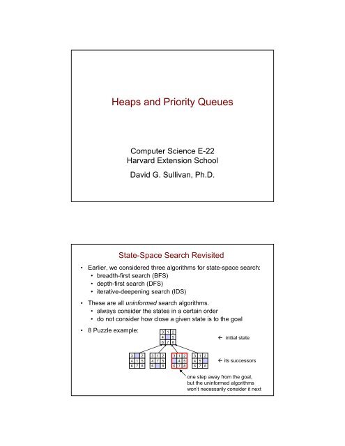
State-Space Search Revisited
• Earlier, we considered three algorithms for state-space search:
• breadth-first search (BFS)
• depth-first search (DFS)
• iterative-deepening search (IDS)
• These are all uninformed search algorithms.
• always consider the states in a certain order
• do not consider how close a given state is to the goal
• 8 Puzzle example: 3 1 2
4 5
6 7 8
initial state
3 2
4 1 5
6 7 8
3 1 2
4 7 5
6 8
3 1 2
4 5
6 7 8
3 1 2
4 5
6 7 8
its successors
one step away from the goal,
but the uninformed algorithms
won’t necessarily consider it next

Informed State-Space Search
• Informed search algorithms attempt to consider more promising
states first.
• These algorithms associate a priority with each successor state
that is generated.
• base priority on an estimate of nearness to a goal state
• when choosing the next state to consider, select the one
with the highest priority
• Use a priority queue to store the yet-to-be-considered search
nodes. Key operations:
• insert: add an item to the priority queue, ordering it
according to its priority
• remove: remove the highest priority item
• How can we efficiently implement a priority queue?
• use a type of binary tree known as a heap
Complete Binary Trees
• A binary tree of height h is complete if:
• levels 0 through h – 1 are fully occupied
• there are no “gaps” to the left of a node in level h
• Complete:
• Not complete ( = missing node):

Representing a Complete Binary Tree
• A complete binary tree has a simple array representation.
• The nodes of the tree are stored in the
array in the order in which they would be
visited by a level-order traversal
(i.e., top to bottom, left to right).
a[0]
a[1] a[2]
a[3] a[4] …
• Examples:
26
10 8 17 14 3
12
32
10
4 18
28
8
17
26 12 32 4 18 28
14 3
Navigating a Complete Binary Tree in Array Form
• The root node is in a[0]
• Given the node in a[i]:
• its left child is in a[2*i + 1]
• its right child is in a[2*i + 2]
• its parent is in a[(i – 1)/2]
(using integer division)
a[0]
a[1]
a[2]
a[3] a[4]
…
a[5]
a[6]
• Examples:
• the left child of the node in a[1] is in a[2*1 + 1] = a[3]
• the right child of the node in a[3] is in a[2*3 + 2] = a[8]
• the parent of the node in a[4] is in a[(4– 1)/2] = a[1]
• the parent of the node in a[7] is in a[(7–1)/2] = a[3]
a[7]
a[8]

Heaps
• Heap: a complete binary tree in which each interior node is
greater than or equal to its children
• Examples:
28
18
12
16
20
8
2
7 10
12 8
5
3 7
• The largest value is always at the root of the tree.
• The smallest value can be in any leaf node – there’s no
guarantee about which one it will be.
• Strictly speaking, the heaps that we will use are max-at-top
heaps. You can also define a min-at-top heap, in which every
interior node is less than or equal to its children.
An Interface for Objects That Can Be Compared
• The Comparable interface is a built-in generic Java interface:
public interface Comparable {
public int compareTo(T other);
}
• It is used when defining a class of objects that can be ordered.
• Classes that implement Comparable include a
compareTo () method that defines the ordering by returning:
• -1 if the called object "comes before" the other object
• 1 if the called object "comes after" the other object
• 0 if the two objects are equivalent in the ordering
• numeric comparison comparison using compareTo
item1 < item2 item1.compareTo(item2) < 0
item1 > item2 item1.compareTo(item2) > 0
item1 == item2 item1.compareTo(item2) == 0

A Class for Items in a Priority Queue
public class PQItem implements Comparable {
private Object data;
private double priority;
...
}
public int compareTo(PQItem other) {
// error-checking goes here…
double diff = priority – other.priority;
if (diff > 1e-6)
return 1;
else if (diff < -1e-6)
return -1;
else
return 0;
}
• We define the compareTo method to return:
• -1 if the calling object has a lower priority than the other object
• 1 if the calling object has a higher priority than the other object
• 0 if they have the same priority
Heap Implementation
public class Heap {
private T[] contents;
private int numItems;
public Heap(int maxSize) {
contents = (T[])new Comparable[maxSize];
numItems = 0;
}
…
}
28
contents
numItems 6
16 20
28 16 20 12 8 5
a Heap object
12 8 5
• Heap is another example of a generic collection class.
• as usual, T is the type of the elements
• extends Comparable specifies T must implement
Comparable
... ...
• must use Comparable (not Object) when creating the array

Heap Implementation (cont.)
public class Heap {
private T[] contents;
private int numItems;
}
…
28
16 20
12 8 5
contents
numItems 6
a Heap object
28 16 20 12 8 5
... ...
• The picture above is a heap of integers:
Heap myHeap = new Heap(20);
• works because Integer implements Comparable
• could also use String or Double
• For a priority queue, we can use objects of our PQItem class:
Heap pqueue = new Heap(50);
Removing the Largest Item from a Heap
• Remove and return the item in the root node.
• In addition, we need to move the largest remaining item to the
root, while maintaining a complete tree with each node >= children
• Algorithm:
1. make a copy of the largest item
2. move the last item in the heap
to the root
3. “sift down” the new root item
until it is >= its children (or it’s a leaf)
4. return the largest item
28
20
16 8 5
12
sift down
the 5:
5
20
20
20
12
5
12
16
12
16 8
16 8
5 8

Sifting Down an Item
• To sift down item x (i.e., the item whose key is x):
1. compare x with the larger of the item’s children, y
2. if x < y, swap x and y and repeat
• Other examples:
sift down
the 10: 10
18
7
18
7
10
3 5
8 6
3 5
8 6
sift down
the 7:
7
26
26
26
23
7
23
18
23
15 18
10
15 18
10
15 7
10
siftDown() Method
private void siftDown(int i) {
T toSift = contents[i];
int parent = i;
int child = 2 * parent + 1;
while (child < numItems) {
// If the right child is bigger, compare with it.
if (child < numItems - 1 &&
contents[child].compareTo(contents[child + 1]) < 0)
child = child + 1;
if (toSift.compareTo(contents[child]) >= 0)
break; // we’re done
// Move child up and move down one level in the tree.
contents[parent] = contents[child];
parent = child;
}
child = 2 * parent + 1;
}
contents[parent] = toSift;
• We don’t actually swap
items. We wait until the
end to put the sifted item
in place.
18
15 7
26
10
23
0 1 2 3 4 5
26 18 23 15 7 10
toSift: 7
parent child
0 1
1 3
1 4
4 9

public T remove() {
T toRemove = contents[0];
remove() Method
contents[0] = contents[numItems - 1];
numItems--;
siftDown(0);
}
return toRemove;
28
5
20
20
12
20
12
16
12
16 8
5
16 8
5 8
0 1 2 3 4 5
28 20 12 16 8 5
numItems: 6
toRemove: 28
0 1 2 3 4 5
5 20 12 16 8 5
numItems: 5
toRemove: 28
0 1 2 3 4 5
20 16 12 5 8 5
numItems: 5
toRemove: 28
Inserting an Item in a Heap
• Algorithm:
1. put the item in the next available slot (grow array if needed)
2. “sift up” the new item
until it is

insert() Method
public void insert(T item) {
if (numItems == contents.length) {
// code to grow the array goes here…
}
contents[numItems] = item;
siftUp(numItems);
numItems++;
}
20
20
35
16
12
16
12
16
20
5 8
5 8
35
5 8
12
0 1 2 3 4 5
20 16 12 5 8
numItems: 5
item: 35
0 1 2 3 4 5
20 16 12 5 8 35
numItems: 5
item: 35
0 1 2 3 4 5
35 16 20 5 8 12
numItems: 6
Converting an Arbitrary Array to a Heap
• Algorithm to convert an array with n items to a heap:
1. start with the parent of the last element:
contents[i], where i = ((n – 1) – 1)/2 = (n – 2)/2
2. sift down contents[i] and all elements to its left
• Example:
0 1 2 3 4 5 6
5 16 8 14 20 1 26
5
16
14 20
8
1 26
• Last element’s parent = contents[(7 – 2)/2] = contents[2].
Sift it down:
5
5
16
8
16
26
14 20
1 26
14 20
1 8

Converting an Array to a Heap (cont.)
• Next, sift down contents[1]:
5
5
16
26
20
26
14 20
1 8
14 16
1 8
• Finally, sift down contents[0]:
5
26
26
20
26
20
5
20
8
14 16
1 8
14 16
1 8
14 16
1 5
Creating a Heap from an Array
public class Heap {
private T[] contents;
private int numItems;
...
public Heap(T[] arr) {
// Note that we don't copy the array!
contents = arr;
numItems = arr.length;
makeHeap();
}
private void makeHeap() {
int last = contents.length - 1;
int parentOfLast = (last - 1)/2;
for (int i = parentOfLast; i >= 0; i--)
siftDown(i);
}
...
}

Time Complexity of a Heap
5
16
14 20
8
1 26
• A heap containing n items has a height

Heapsort
public class HeapSort {
public static void
heapSort(T[] arr) {
// Turn the array into a max-at-top heap.
Heap heap = new Heap(arr);
int endUnsorted = arr.length - 1;
while (endUnsorted > 0) {
// Get the largest remaining element and put it
// at the end of the unsorted portion of the array.
T largestRemaining = heap.remove();
arr[endUnsorted] = largestRemaining;
}
}
}
endUnsorted--;
• We define a generic method, with a type variable in the method
header. It goes right before the method's return type.
• T is a placeholder for the type of the array.
• can be any type T that implements Comparable.
• Sort the following array:
Heapsort Example
• Here’s the corresponding complete tree:
13
0 1 2 3 4 5 6
13 6 45 10 3 22 5
6
45
10 3
22 5
• Begin by converting it to a heap:
sift down
45
6
13
45
sift down
6
10
13
45
sift down
13
10
45
22
10 3
22 5
6 3
22 5
6 3
13 5
no change, because
45 >= its children

Heapsort Example (cont.)
• Here’s the heap in both tree and array forms:
10
45
22
0 1 2 3 4 5 6
45 10 22 6 3 13 5
endUnsorted: 6
6 3
13 5
• Remove the largest item and put it in place:
remove()
copies 45;
moves 5
to root
10
45
5
22
remove()
sifts down 5;
returns 45
10
22
heapSort() puts 45 in place;
decrements endUnsorted
13
10
22
13
6 3 13
5
6 3
5
6 3
5
toRemove: 45
0 1 2 3 4 5 6
22 10 13 6 3 5 5
endUnsorted: 6
largestRemaining: 45
0 1 2 3 4 5 6
22 10 13 6 3 5 45
endUnsorted: 5
copy 22;
move 5
to root
10
22 5
13
Heapsort Example (cont.)
sift down 5;
return 22
10
13
5
put 22
in place
10
13
5
6 3
5
6 3
6 3
copy 13;
move 3
to root
toRemove: 22
10
13 3
5
sift down 3;
return 13
0 1 2 3 4 5 6
13 10 5 6 3 5 45
endUnsorted: 5
largestRemaining: 22
6
10
5
put 13
in place
0 1 2 3 4 5 6
13 10 5 6 3 22 45
endUnsorted: 4
6
10
5
6 3
toRemove: 13
3
0 1 2 3 4 5 6
10 6 5 3 3 22 45
endUnsorted: 4
largestRemaining: 13
3
0 1 2 3 4 5 6
10 6 5 3 13 22 45
endUnsorted: 3

copy 10;
move 3
to root
6
10 3
5
Heapsort Example (cont.)
sift down 3;
return 10
6
3 5
put 10
in place
6
3 5
3
copy 6;
move 5
to root
toRemove: 10
65
3 5
sift down 5;
return 6
0 1 2 3 4 5 6
6 3 5 3 13 22 45
endUnsorted: 3
largestRemaining: 10
3
5
put 6
in place
0 1 2 3 4 5 6
6 3 5 10 13 22 45
endUnsorted: 2
3
5
toRemove: 6
0 1 2 3 4 5 6
5 3 5 10 13 22 45
endUnsorted: 2
largestRemaining: 6
0 1 2 3 4 5 6
5 3 6 10 13 22 45
endUnsorted: 1
copy 5;
move 3
to root
3
35
Heapsort Example (cont.)
sift down 3;
return 5
3 put 5
3
in place
toRemove: 5
0 1 2 3 4 5 6
3 3 6 10 13 22 45
endUnsorted: 1
largestRemaining: 5
0 1 2 3 4 5 6
3 5 6 10 13 22 45
endUnsorted: 0

How Does Heapsort Compare?
algorithm best case avg case worst case extra
memory
selection sort O(n 2 ) O(n 2 ) O(n 2 ) O(1)
insertion sort O(n) O(n 2 ) O(n 2 ) O(1)
Shell sort O(n log n) O(n 1.5 ) O(n 1.5 ) O(1)
bubble sort O(n 2 ) O(n 2 ) O(n 2 ) O(1)
quicksort O(n log n) O(n log n) O(n 2 ) O(1)
mergesort O(n log n) O(n log n) O(nlog n) O(n)
heapsort O(n log n) O(n log n) O(nlog n) O(1)
• Heapsort matches mergesort for the best worst-case time
complexity, but it has better space complexity.
• Insertion sort is still best for arrays that are almost sorted.
• heapsort will scramble an almost sorted array before sorting it
• Quicksort is still typically fastest in the average case.
State-Space Search: Estimating the Remaining Cost
• As mentioned earlier, informed search algorithms associate a
priority with each successor state that is generated.
• The priority is based in some way on the remaining cost –
i.e., the cost of getting from the state to the closest goal state.
• for the 8 puzzle, remaining cost = # of steps to closest goal
• For most problems, we can’t determine the exact remaining cost.
• if we could, we wouldn’t need to search!
• Instead, we estimate the remaining cost using a heuristic function
h(x) that takes a state x and computes a cost estimate for it.
• heuristic = rule of thumb
• To find optimal solutions, we need an admissable heuristic –
one that never overestimates the remaining cost.

Heuristic Function for the Eight Puzzle
• Manhattan distance = horizontal distance + vertical distance
• example: For the board at right, the
Manhattan distance of the 3 tile
from its position in the goal state
= 1 column + 1 row = 2
4 3 1
7 2
6 8 5
1 2
3 4 5
6 7 8
goal
• Use h(x) = sum of the Manhattan distances of the tiles in x
from their positions in the goal state
• for our example:
2 units away
2 units away
1 unit away
4 3 1
1 unit away 7 2 1 unit away
0 units away
6 8 5
1 unit away
1 unit away
h(x) = 1 + 1 + 2 + 2
+ 1 + 0 + 1 + 1 = 9
• This heuristic is admissible because each of the operators
(move blank up, move blank down, etc.) moves a single tile a
distance of 1, so it will take at least h(x) steps to reach the goal.
Greedy Search
• Priority of state x, p(x) = -1 * h(x)
• mult. by -1 so states closer to the goal have higher priorities
3 2
4 1 5
6 7 8
h = 3
p = -3
3 1 2
4 7 5
6 8
h = 3
p = -3
3 1 2
4 5
6 7 8
3 1 2
4 5
6 7 8
h = 1
p = -1
3 1 2
4 5
6 7 8
h = 3
p = -3
initial state
its successors
heuristic values and
priorities
• Greedy search would consider the highlighted successor before
the other successors, because it has the highest priority.
• Greedy search is:
• incomplete: it may not find a solution
• it could end up going down an infinite path
• not optimal: the solution it finds may not have the lowest cost
• it fails to consider the cost of getting to the current state

A* Search
• Priority of state x, p(x) = -1 * (h(x) + g(x))
where g(x) = the cost of getting from the initial state to x
3 1 2
4 5
6 7 8
3 2
4 1 5
6 7 8
h = 3
p = -(3 + 1)
3 1 2
4 7 5
6 8
h = 3
p = -(3 + 1)
3 1 2
4 5
6 7 8
h = 1
p = -(1 + 1)
3 1 2
4 5
6 7 8
h = 3
p = -(3 + 1)
3 2
4 1 5
6 7 8
h = 4
p = -(4 + 2)
3 2
4 1 5
6 7 8
h = 4
p = -(4 + 2)
• Incorporating g(x) allows A* to find an optimal solution –
one with the minimal total cost.
• It is complete and optimal.
Characteristics of A*
• provided that h(x) is admissable, and that g(x) increases or stays
the same as the depth increases
• Time and space complexity are still typically exponential in the
solution depth, d – i.e., the complexity is O(b d ) for some value b.
• However, A* typically visits far fewer states than other optimal
state-space search algorithms.
solution
depth
iterative
deepening
A* w/ Manhattan
dist. heuristic
4 112 12
8 6384 25
12 364404 73
16 did not complete 211
20 did not complete 676
Source: Russell & Norvig,
Artificial Intelligence: A Modern
Approach, Chap. 4.
The numbers shown are the
average number of search
nodes visited in 100 randomly
generated problems for each
solution depth.
The searches do not appear to
have excluded previously seen
states.
• Memory usage can be a problem, but it’s possible to address it.

Implementing Informed Search
• Add new subclasses of the abstract Searcher class.
• For example:
public class GreedySearcher extends Searcher {
private Heap nodePQueue;
public void addNode(SearchNode node) {
nodePQueue.insert(
new PQItem(node, -1 * node.getCostToGoal()));
}
…