2015-hindawe- bo quan sat nhieu-Unknown Disturbance Estimation for a PMSM with a Hybrid

188 Journal of Power Electronics, Vol. 9, No. 2, March 2009
JPE 9-2-7
Adaptive Flux Observer with On-line Inductance Estimation of an
Interior PM Synchronous Machine Considering Magnetic Saturation
Yu-Seok Jeong † and Jun-Young Lee *
†* Dept. of Electrical Eng., Myongji University, Korea
ABSTRACT
This paper presents an adaptive flux observer to estimate stator flux linkage and stator inductances of an interior
permanent-magnet synchronous machine considering magnetic saturation. The concept of static and dynamic inductances
due to saturation is introduced in the machine model to describe the relationship between current and flux linkage and the
relationship between their time derivatives. A flux observer designed in the stationary reference frame with constant
inductance is analyzed in the rotor reference frame by a frequency-response characteristic. An adaptive algorithm for an
on-line inductance estimation is proposed and a Lyapunov-based analysis is given to discuss its stability. The dynamic
inductances are estimated by using Taylor approximation based on the static inductances estimated by the adaptive method.
The simulation and experimental results show the feasibility and performance of the proposed technique.
Keywords: Adaptive flux observer, Magnetic saturation, Inductance estimation, Lyapunov-based analysis
1. Introduction
Interior permanent-magnet synchronous machines (IPM
SMs) in automotive applications are typically designed to
have a high saliency ratio under a wide range of operating
conditions [1] . The magnetic characteristics of IPMSM are
such that a lumped parameter model for these machines is
nonlinear due to the saturated dq-axis inductances [2] .
Based on the voltage equation of an IPMSM, its
electrical system can be expressed as a dual-input-dualoutput
(DIDO) system, where the inputs and outputs are
the stator voltages and the stator currents respectively. As
Manuscript received June 23, 2008; revised Dec. 18, 2008
† Corresponding Author: jeong@mju.ac.kr
Tel: +82-31-330-6363, Fax: +82-31-321-0271, Myongji Univ.
* Dept. of Electrical Eng., Myongji University, Korea
parameters in this system, the stator resistance and the
rotor-magnet flux linkage vary with temperature and the
inductances vary with currents. The motor speed has been
typically considered a slowly time-varying parameter
rather than another state variable assuming that dynamics
of the mechanical system is much slower than that of the
electrical system.
Most research done on an observer in PMSM drive
contribute to position estimation or load torque estimation
in a sensorless control [3]-[5] . The stator inductances used in
the flux observer are typically constants assuming no
saturation, or are taken from two-dimensional (2D)
look-up tables from motor characteristics to consider the
saturation effect [6] . The estimated flux for sensorless
control is processed to generate the position error in a
position observer. With a position sensor, the flux
observer can be used to estimate another machine’s

Adaptive Flux Observer with On-line Inductance Estimation of … 189
parameters rather than the rotor position. Recently, an
on-line inductance estimation scheme with a position
sensor was introduced to improve the decoupling
characteristics of a current controller designed in the rotor
reference frame for an IPMSM drive [7] . This estimation
technique is based on the voltage equation in a steady state
and utilized the inverse of speed and current, which is not
desirable when the machine operates at low speed or in
light load.
This paper proposes an adaptive flux observer with
on-line inductance estimation for an IPMSM with a
position sensor. The flux observer is designed in the
stationary reference frame rather than in the rotor
reference frame to reduce the effect of inductance
variation due to magnetic saturation on the estimation
accuracy in steady state. The estimation error in the flux
observer is transformed to that in the rotor reference frame
and utilized to identify inductance variation in real time.
2. Mathematical Model of IPMSM Considering
Magnetic Saturation
The flux linkage model of an IPMSM and its time
derivative in the rotor reference frame can be generally
written as
r r
λ
dq
= Lsidq
+ Λ , d r d r
m λ
dq
= Ldq
i
(1)
dq
dt dt
r
where λ and r dq
i denote the stator flux linkage vector
dq
and the stator current vector respectively. Static
inductances, dynamic inductances and magnet flux linkage
in (1) can be defined by
L s
L dq
⎡
r
λd
⎢
= ⎢
r
⎢λq
⎢
⎢⎣
r r
r r r r r
( i ,0) − λ ( 0,0) λd
( id
, iq
) − λd
( id
,0)
d
q
r r r r r r r
( i , i ) − λ ( 0, i ) λ ( 0, i ) − λ ( 0,0)
d
r
⎡∂λd
⎢ r
⎢
∂ id
= r
⎢∂λq
⎢ r
⎢⎣
∂ id
d
i
r
q
r
id
d
q
r
∂λ ⎤
d
r ⎥
∂iq
⎥ ,
r
∂λq
⎥
r ⎥
∂ iq
⎥⎦
q
Λ m
q
⎡ r
⎢ λd
= ⎢
⎢ r
λ
⎢
q
⎣
i
r
q
r
iq
( 0,0)
⎤
q
( )
⎥ ⎥⎥ 0,0 ⎥
⎦
⎤
⎥
⎥ ,
⎥
⎥
⎥⎦
(2)
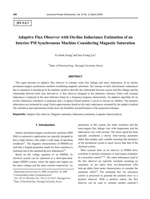
The flux linkages of a test machine in this work with
respect to the currents in the rotor reference frame are
depicted in Fig. 1, where it can be seen that the saturation
effect on the q-axis is more conspicuous than on the
d-axis.
r
λ d
( Wb)
( Wb)
0 .4
0 .4
0 .2
0 .2
0
0
− 0 .2
− 0 .2
− 0 .4
− 0 .4
0
0
− 100
300
( A ) − 200
− 300 100 200 − 100
r
r
i
− 200
d
r i
0 i q
( A )
( A )
d − 300 0
r
λ q
300
200
100
r
( A )
(a)
(b)
Fig. 1 d-q flux linkage in the rotor reference frame
(a) d-axis flux linkage (b) q-axis flux linkage
Neglecting the cross magnetization unless the current is
extremely high, the flux linkage only depends on the
corresponding axis current in the rotor reference frame
and the static and the dynamic inductances become
diagonal.
L s
where
L
qq
⎡ L
ds
= ⎢
⎣ 0
L
dλ
= .
di
r
q
r
q
0 ⎤
L
⎥
qs ⎦
λ
,
− Λ
L dq
r
d m
ds
= ,
r
id
⎡ L
dd
= ⎢
⎣ 0
L
qs
0 ⎤
L
⎥
qq ⎦
λ
= ,
i
r
q
r
q
L
dd
i q
r
d
r
d
(3)
dλ
= and
di
The stator voltage model of an IPMSM in the stationary
reference frame can be expressed by
v
s
dq
s d
R s
i
dq
+ λ
dt
=
(4)
s
dq
where R denotes the stator resistance.
s
The transformation between the stationary reference
frame and the rotor reference frame can be expressed by
cosθ
− sin θ
R θ =
.
r ⎢
⎣sin
θr
cosθr
the rotation matrix ⎡ r
r ⎤
( ) ⎥ ⎦
3. Flux Observer
A flux observer designed in the stationary reference
frame can be expressed by

190 Journal of Power Electronics, Vol. 9, No. 2, March 2009
v
s
dq
s s
( i − ˆi
)
ˆ s d s
= R idq
λˆ
s
+
dq
− K
(5)
o dq dq
dt
where the circumflex denotes an estimated parameter/
variable and K denotes an observer gain matrix.
o
The observer block diagram is depicted in Fig. 2(a) and
can be converted to its equivalent form in Fig. 2(b) by
setting K = ωo
( θr
) ˆ R −1
o
R Ls
( θr
) as a time-varying gain.
This yields
v
s
dq
= Rˆ
= Rˆ
= Rˆ
= Rˆ
i
s
s dq
i
s
s dq
i
s
s dq
i
s
s dq
d
+ λˆ
dt
d
+ λˆ
dt
d
+ λˆ
dt
d
+ λˆ
dt
s
dq
s
dq
s
dq
s
dq
− ω R
− ω R
− ω R
− ω
o
o
o
o
s s
( ) Lˆ
−1
θ
sR
( )( i ˆ
r
θr
dq
− idq
)
r r
( θ ) Lˆ
s
( i ˆ
r dq
− idq
)
s r
( ){ Lˆ
−1
θ R ( θ ) i − ( λˆ
− Λˆ
)}
r
s
s
s
[ R( ){ Lˆ
−1
θ R ( θ ) i + Λˆ
} − λˆ
]
r
s
r
r
dq
dq
dq
m
m
dq
(6)
Defining two estimated fluxes, one is from a voltage
s s s
λˆ = v − ˆ i dt and the other is from a cur-
∫
model ( )
v
dq
R s
dq
s
{ i + Λˆ
}
s
rent model λˆ R( ) Lˆ
−1
= θ R ( θ )
i
r
s
r
dq
m
. The closed-
loop estimated flux with respect to these in a frequency
domain can be expressed by
λˆ
s
dq
s s
s
λˆ
ωo
=
v
+ λˆ
(7)
i
s + ω s + ω
o
o
The estimated flux basically consists of the high-passfiltered
flux from the voltage model and the low-passfiltered
flux from the current model. Thus in steady state it
follows the current model at low frequency and the
voltage model at high frequency with the crossover
frequency ω . Since this feature makes the flux observer
o
robust to inductance variation at high frequency, the flux
observer is preferred to be designed in the stationary
reference frame rather than in the rotor reference frame [8] .
Even though the flux observer is designed in the
stationary reference frame, its dynamic characteristics in a
frequency domain can be analyzed in the rotor reference
frame. Transforming (4) and (6) to the rotor reference
frame and applying the Laplace transform yields
s
v dq
1
s
R s
Rˆ
s
1
s
s
λ dq
s
i dq
s
λˆ dq
−1
1
R ( )
( )
θ r
−1
R ( θ r
)
Λ m
L − s
Λˆ
m
1
R θ r
L − s
R( θ r
)
λˆ
r
dq
×
=
( sI
+ ω J + ω I)
−1
r
[{ I J ( I ˆ I Lˆ
−1
s + ωr
+ Rs
− Rs
+ ωo
s
) L
s
} λ
( I ˆ I Lˆ
−1
− R − R + ω ) L Λ + ω Λˆ
]
where
⎡0
−1⎤
J = .
⎢ ⎥
⎣1
0 ⎦
s
r
s
o
o
s
s
m
o
m
dq
(8)
K o
s
v dq
1
s
R s
Rˆ
s
1
s
s
λ dq
s
λˆ
v
s
i dq
(a)
−1
1
R ( )
L −
( )
θ r
Λ m
s
R θ r
−1
R ( θ r
) Lˆ
R( θ r
)
s
Λˆ
m
λˆ s dq
ω o
s
(b)
Fig. 2 Flux observer in the stationary reference frame
(a) original form (b) equivalent form
s
λˆ i
It can be seen that the transfer matrix becomes the unity
without parameter variation.
The steady-state characteristic of the flux observer can
also be analyzed by using complex vector notations.
Substituting s = 0 and in (8) and using the relationship
r
r r
r
r r
Λ
d
= 0.
5( Λ
dq
+ Λdq
) and Λ
q
= − j0.
5( Λ
dq
− Λdq
) to obtain
complex vector expression yields
Λˆ
G
r
dq
λ
= G
( jω
)
r
λ
r
r
( jω
) Λ + G ( jω
) Λ + G ( jω
)
r
dq
R ⎛
s
Rˆ
⎞ ⎛
s ⎜
1 1
⎜ ⎟
1 −
+
2 R
⎝ s ⎠ ⎝ L
ds
L
qs
=
ω
λ
r
dq
o
Λ
⎞
⎟
ω
+
⎠ 2
+ jω
r
o
r
⎛ Lˆ
⎜
⎝
L
ds
ds
Λ
m
Lˆ
+
L
qs
qs
⎞
⎟ + jω
r
⎠

Adaptive Flux Observer with On-line Inductance Estimation of … 191
G
λ
( jω
)
r
=
R
s
2
⎛ Rˆ
⎜
1 −
⎝ R
s
s
⎞ ⎛
⎟ ⎜
1
⎠ ⎝ L
ds
1
−
L
ω +
o
qs
⎞ ω ⎛
o ⎜ Lˆ
⎟ +
⎜
⎠ 2
⎝
L
jω
r
ds
ds
Lˆ
−
L
qs
qs
⎞
⎟
⎟
⎠
of the transfer function, it is analyzed using the matrix
norm of the transfer matrix in a multi-input-multi-output
(MIMO) system.
G
Λ
( jω
)
where
r
R
L
= −
r
dq
s
ds
⎛ Rˆ
⎞ ⎛
s
Lˆ
⎜ ⎟ ω ⎜
1 − +
o
R
⎝ s ⎠ ⎝ L
ω + jω
r
r
Λˆ , Λ and Λ
dq
o
dq
r
ds
ds
Λˆ
−
Λ
m
m
⎞
⎟
⎠
(9)
denote the estimated flux
vector, the actual flux vector, and the conjugate flux
vector in steady state, respectively. It should be noted that
the conjugate expression comes from the inherent saliency
of an IPMSM. The geometric interpretation of (9) in the
DQ plane is shown in Fig. 3.
The sensitivity of the flux observer to parameter
variation can be analyzed from the transfer matrix in (8).
S
S
S
Rs
Lds
Lqs
= σ
= σ
= σ
max
max
max
T
[ SR
( jω)
] = λ [ ( − jω) ( jω)
]
s
max
SR
S
s
Rs
T
[ S
L
( jω)
] = λ [ ( − jω) ( jω)
]
ds
max
SL
S
ds
Lds
T
[ S ( jω)
] = λ [ S ( − jω) S ( jω)
]
Lqs
max
Lqs
Lqs
(11)
λ max
denote the maximum singular
value and the maximum eigenvalue, respectively.
where σ max
[ ⋅ ] and [ ⋅ ]
10
S R s
S
S
S
Rs
Lds
Lqs
= R
s
= L
= L
{( s + ω ) I + ω J}
ds
qs
o
−1
{( s + ω ) I + ω J}
o
−1
−1
s
ω L
∂
∂L
∂
∂L
−1
s
−1
−1
{( s + ω ) I + ω J} ω L L
o
r
r
r
r
λ q
L
o
o
s
s
ds
qs
L
s
(10)
Magnitude (dB)
−10
− 30
− 50
10
0
15
150
1500
1
10
( r /min)
( r / min)
( r /min)
2
10
Frequency (Hz)
3
10
(a)
L
ds
+ L
2
qs
I
r
dq
L
+
G
ds
Λ
− L
2
qs
I
r
dq
( jωr
) Λm
r
Λˆ
dq
G
λ
r
( jω
) Λ
r dq
r
Λ dq
10
S ,
S
Lds L qs
G
λ
r
( jω
) Λ
r
dq
r
Λ dq
Λ m
r
λ d
Magnitude (dB)
−10
− 30
− 50
10
0
15
150
1500
1
10
( r / min)
( r / min)
( r / min)
2
10
3
10
Fig. 3 Estimated steady-state flux vector
Frequency (Hz)
(b)
While the sensitivity in a single-input-single-output
(SISO) system is typically analyzed using the magnitude
Fig. 4 Sensitivity of the flux observer to parameter variation
(a) resistance sensitivity (b) inductance sensitivity

192 Journal of Power Electronics, Vol. 9, No. 2, March 2009
For the test motor with its parameters in Table 1, the
sensitivity of the flux observer to parameter variation with
the crossover frequency ωo = 20π
rad/sec is depicted in
Fig. 4. The resistance sensitivity is shown in Fig. 4(a) and
is almost constant below the crossover frequency, reaches
its peak at the operating frequency and is declined as the
frequency increases. This feature depending on the
operating speed is based on the transformation between
the reference frames. The inductance sensitivity is shown
in Fig. 4(b) and is similar to the resistance sensitivity. A
decrease of the sensitivity to parameter variation at a high
operating speed is due to a lesser effect on the estimated
flux from the open-loop voltage model. It should be noted
that increasing the order of the transfer matrix results in
less sensitivity to resistance variation at low operating
speed but more sensitivity to inductance variation at high
operating speed [9] .
4. Inductance Estimation
The static inductance can be estimated by using the
estimation error transformed to the rotor reference frame.
The error dynamics of the flux observer can be derived
from (4) and (6).
d s
s
1
∆λdq
= −ωo∆λ
dq
+ ωoR
dt
− ∆R
i
s
s dq
+ ω R
o
−
( θr
) ∆LsR
( θr
)
( θ ) ∆Λm
r
i
s
dq
(12)
s s s
where ∆ λ
dq
= λ
dq
− λˆ
,
dq
∆ Rs
= Rs
− Rˆ
,
s
∆ Ls
= Ls
− Lˆ
,
s
and ∆ Λm
= Λm
− Λˆ
. In the left side of (12), the 1 st term
m
is related to the state variable, the 2 nd term to input, and
other terms is treated as disturbance.
A positive definite function can be defined by
s T
dq
s
dq
T −1
( ∆L
Γ ∆L
)
V = ∆λ
∆λ
+ ωo tr
(13)
s
where tr denotes a trace of a matrix, and this function
becomes a Lyapunov-like function since the input variable
in (12), i.e. the current is another state variable to be
controlled.
An input coefficient in the error dynamics is typically
estimated by the multiplication of estimation error and
input [10] . It should be noted that the estimation error of the
s
current should be used since that of the flux linkage is not
available. Therefore the adaptive law for inductance
estimation can be described by
d
dt
∆L
s
= Γ L
= Γ
= Γ
ˆ −1
s
( )( ˆ s s T
s
R θ
r
i
dq
− i
dq
) i
dq
R ( θ
r
)
T
{ ˆ r
( ˆ r ˆ r
λ
dq
− L
si
dq
+ Λ
m
)}
i
dq
r
r
r T
( ∆λ
− ∆L
i − ∆Λ
) i
dq
s dq
m
dq
(14)
where Γ denotes the adaptive gain matrix. It can be seen
that the static inductances are estimated using the
variables in the rotor reference frame. To check the
stability of this adaptive technique, differentiating (13)
yields.
dV
dt
⎛
= ⎜
⎝
= −2
− ∆R
+ ω
d
dt
+ ∆Λ
∆λ
⎪⎧
⎛
+ ω
o
tr ⎨⎜
⎪⎩ ⎝
o
r
r T r
r
ω
o
( ∆λ
dq
− ∆L
si
dq
) ( ∆λ
dq
− ∆L
si
dq
)
r T r
r T r
s
( i
dq
∆λ
dq
+ ∆λ
dq
i
dq
)
r
r T
{( ∆λ
dq
− ∆L
si
dq
) ∆Λ
m
T r
r
( ∆λ
− ∆L
i )}
m
s
dq
d
dt
⎞
⎟
⎠
dq
T
∆λ
s
dq
⎞
∆L
s ⎟
⎠
T
+ ∆λ
Γ
−1
s dq
s T
dq
∆L
+ ∆L
s
⎛
⎜
⎝
d
dt
∆λ
T
s
s
dq
Γ
⎞
⎟
⎠
−1
⎛
⎜
⎝
d
dt
∆L
s
⎞⎪⎫
⎟⎬
⎠⎪⎭
(15)
The time derivative of the Lyapunov-like function in
(13) does not become positive with actual values of the
stator resistance and the rotor magnet flux linkage, which
is hardly achievable. To prevent undesirable blow-up, the
projection method is utilized to estimate inductances with
an adaptive technique.
if Lˆ
ds
< L
or Lˆ
d
Lˆ
dt
d
Lˆ
dt
= L
= γ
= 0
, i
d ˆ r
Lds
= γd
id
dt
d
otherwise Lˆ
ds
= 0
dt
if Lˆ
< L or Lˆ
= L , i
qs
do
qo
otherwise
ds
qs
qs
qs
do
qo
i
r
q q
r
( ˆr
ˆ ˆ r
d
λd
− Λm
− Ldsid
)
( λˆ
r
− Λˆ
− ˆ r
L i )
d
r
( ˆr
ˆ r
q
λq
− Lqsiq
)
( λˆ
r
− ˆ r
L i )
q
m
qs q
ds d
≤ 0
≤ 0
(16)
The adaptive flux observer with on-line inductance esti-

Adaptive Flux Observer with On-line Inductance Estimation of … 193
s
v dq
1
s
R s
Rˆ
s
1
s
s
λ dq
s
λˆ
v
s
i dq
−1
θ r
Λ m
1
L −
s
−1
R ( )
( )
θ r
R θ r
Lˆ
s
R ( ) ×
R( θ r
)
Λˆ
ω o
s
m
s
λˆ dq
Fig. 5 On-line inductance estimation
γ
s
s
λˆ i
×
−1
R ( θ r
)
mation is depicted in Fig. 5. The estimated inductance
which is constant in the previous flux observer is now
updated in real time. It is crucial to check the condition for
persistent excitation when an adaptive scheme is used.
Dynamic inductances are defined by the relationship
between the time derivatives of current and flux linkage in
the rotor reference frame. Therefore it is impossible to
estimate dynamic inductances in steady state using the
definition in (1). An estimation method using Taylor
approximation of flux linkage is developed.
λ
r
dq
r
( i )
dq
( 0, 0)
( 0, 0)
r
⎡λd
= ⎢ r
⎢⎣
λq
r
1 ⎡i
+ ⎢ r
2 ⎢⎣
i
T
dq
T
dq
⎤ ⎡i
⎥ + ⎢
⎥⎦
⎢⎣
i
2 r
∇ λd
2 r
∇ λ
q
r T
dq
r T
dq
r
∇λ
r
∇λ
( 0, 0)
( 0, 0)
d
q
i
i
( 0, 0)
( 0, 0)
r
dq
r
dq
⎤
⎥ +
⎥⎦
⎤
⎥
⎥⎦
L
(17)
Neglecting cross magnetization and using the definition
of inductances in (3), the dynamic inductance can be
estimated from the static inductance.
Lˆ
dq
r
⎡ d λ
d
⎢ r
≈ ⎢
di
d
⎢
⎢ 0
⎣
( 0 )
0
r
d λ
q
r
di
q
⎤
⎥
⎥
⎥
⎥
⎦
( 0 )
− 1
Lˆ
5. Simulation and Experiment
2
s
(18)
The adaptive flux observer with on-line inductance
estimation has been investigated by computer simulations
and lab experiments. Simulink® was used for the
computer simulation. The IPMSM used in this simulation
and experiment is an integrated starter/alternator for
automotive applications.
Table 1 Nominal machine parameters
Symbol Description Value (Unit)
P rated Rated Power 5 (kW)
V rated Rated Voltage 30 (Vrms)
I rated Rated Current 150 (Arms)
P Pole pairs 4 (n.u.)
R s Stator resistance 13 (mΩ)
L ds D-axis inductance 90 (µH)
L qs Q-axis inductance 290 (µH)
Λ m Magnet flux linkage 11 (mV·sec)
The nominal parameters of this machine are shown in
Table 1. The test condition is the torque command of 30
Nm at three different speeds of 15 r/min, 150 r/min, and
1500 r/min which correspond to 1 Hz, 10 Hz, and 100 Hz,
respectively. The crossover frequency of the flux observer
is set to 20π rad/sec which corresponds to 10 Hz.
The simulation result for the flux observer without
inductance estimation is depicted in Fig. 6. The upper
figures in (a), (b), and (c) show the calculated flux from
the look-up table and the estimated flux from the flux
observer on d-axis. The lower figures show those on
q-axis. The estimation accuracy at low speed shown in (a)
is worse on q-axis, since magnetic saturation makes more
of an effect on q-axis. The estimation accuracy at the
crossover frequency shown in (b) becomes better on
q-axis, but worse on d-axis since it has the most
cross-coupling effect at this speed. The estimation
accuracy at high speed shown in (c) becomes better on
both axes since the flux is estimated dominantly from the
voltage model, which takes no effect from inductance
variation. The characteristic of the flux observer with
inductance estimation is depicted in Fig. 7. The estimation
accuracy is improved particularly at low speed. The
inductance estimation using the proposed adaptive law is
shown in Fig. 8.
The test setup employs a TI’s DSP-based controller
with the sampling time of 0.1ms for the current control.
The experiments under the same condition are depicted for
the flux observer without inductance estimation in Fig. 9,
for the flux observer with inductance estimation in Fig. 10,
and for the inductance estimation by the adaptive law in
Fig. 11. It matches well with the simulation results, except
for periodic ripples at high speed. These ripples having
operating frequency are caused from the periodic position
errors in synchronization with the rotation cycle of the
resolver that occur due to its structure [11] .

194 Journal of Power Electronics, Vol. 9, No. 2, March 2009
20
20
20
10
r ˆr
λ d , λ d 0
( mV sec )
−10
r
λ d
r λˆd
10
r ˆr
λ d , λ d
0
( mV sec)
−10
r λˆ
d
r
λ d
10
r ˆr
λ d , λ d
0
( mV sec )
−10
r
λ d
r
λˆ
d
− 20
− 20
− 20
60
40
r λˆ
q
60
40
λˆ
r
q
60
40
r
λˆ
q
λ r
, λ ˆr
q q
( mV sec )
20
r λ q
λ r
, λ ˆr
q q
( mV sec)
20
r λ
q
λ r
, λ ˆr
q q
( mV sec )
20
r λ
q
0
0
0
− 20
0
time(m sec )
10 0
− 20
0
ti me (msec)
10 0
− 20
0
time(mse c)
(a) (b) (c)
Fig. 6 Estimation characteristics of the flux observer without inductance estimation (simulation)
(a) 30 Nm command at 15 r/min (b) 30 Nm command at 150 r/min (c) 30 Nm command at 1500 r/min
100
20
20
20
10
10
10
r ˆr
λ d , λ d
( mV sec )
0
λˆ r
d
r
λ d
r ˆr
λ d , λ d
( mV sec )
0
λ
r
d
r
λˆd
r ˆr
λ d , λ d
( mV sec )
0
r
λ d
r λˆ d
−10
− 20
60
40
λ r
, λ ˆr
q q
20
( mV sec )
r λ
q
r
λˆq
−10
− 20
60
40
λ r
, λ ˆr
q q
20
( mV sec )
r λ
q
r
λˆq
−10
− 20
60
40
λ r
, λ ˆr
q q
20
( mV sec )
r λ
q
r
λˆq
0
0
0
− 20
0
time(mse c)
100
− 20
0
time(mse c)
100
− 20
0
time(mse c)
(a) (b) (c)
Fig. 7 Estimation characteristics of the flux observer with inductance estimation (simulation)
(a) 30 Nm command at 15 r/min (b) 30 Nm command at 150 r/min (c) 30 Nm command at 1500 r/min
100
200
200
200
100
r i q
100
r i q
100
r i q
r r
i i
q
( A)
d ,
0
r r
i i
q
( A)
d ,
0
r r
i i
q
( A)
d ,
0
−100
r
i d
−100
r
i d
−100
r
i d
− 200
− 200
− 200
400
400
400
300
300
300
Lˆ
, Lˆ
ds
( µ H)
qs
200
100
Lˆ qs
Lˆ
ds
Lˆ
, Lˆ
ds
( µ H)
qs
200
100
Lˆ qs
Lˆ
ds
Lˆ
, Lˆ
ds
( µ H)
qs
200
100
Lˆ qs
Lˆ
ds
0
0
time(mse c)
100
0
0
time(mse c)
100
0
0
time(mse c)
(a) (b) (c)
Fig. 8 On-line inductance estimation using the proposed adaptive method (simulation)
(a) 30 Nm command at 15 r/min (b) 30 Nm command at 150 r/min (c) 30 Nm command at 1500 r/min
100

Adaptive Flux Observer with On-line Inductance Estimation of … 195
20
20
20
10
λ r
, λ ˆr
d d
0
( mV sec)
−10
r
λ d
λˆ
r
d
10
λ r
, λ ˆr
d d
0
( mV sec)
−10
λˆ
r
d
r
λ d
10
λ r
, λ ˆr
d d
0
( mV sec)
−10
r
λ d
λˆ
r
d
− 20
− 20
− 20
60
40
λˆ
r
q
60
40
λˆ
r
q
60
40
λˆ
r
q
r ˆr
λ q
, λq
( mV sec)
20
r
λ q
r ˆr
λ q
, λq
( mV sec)
20
r
λ q
r ˆr
λ q
, λq
( mV sec)
20
r
λ q
0
0
0
− 20
0
time(msec)
100
− 20
0
time(msec)
100
− 20
0
time(msec)
(a) (b) (c)
Fig. 9 Estimation characteristics of the flux observer without inductance estimation (experiment)
(a) 30 Nm command at 15 r/min (b) 30 Nm command at 150 r/min (c) 30 Nm command at 1500 r/min
100
20
20
20
λ r
, λ ˆr
d d
( mV sec)
10
0
r
λ d
λˆ
r
d
λ r
, λ ˆr
d d
( mV sec)
10
0
r
λ d
λˆ
r
d
λ r
, λ ˆr
d d
( mV sec)
10
0
r
λ d
λˆ
r
d
−10
−10
−10
− 20
− 20
− 20
60
60
60
40
40
40
r ˆr
λ q
, λq
( mV sec)
20
r
λ q
λˆ
r
q
r ˆr
λ q
, λq
( mV sec)
20
r
λ q
λˆ
r
q
r ˆr
λ q
, λq
( mV sec)
20
r
λ q
λˆ
r
q
0
0
0
− 20
0
time(msec)
100
− 20
0
time(msec)
100
− 20
0
time(msec)
(a) (b) (c)
Fig. 10 Estimation characteristics of the flux observer with inductance estimation (experiment)
(a) 30 Nm command at 15 r/min (b) 30 Nm command at 150 r/min (c) 30 Nm command at 1500 r/min
100
200
200
200
100
r
i q
100
r
i q
100
r
i q
r r
i iq
( A)
d ,
0
r
i , r
d
iq
( A)
0
r
i , r
d
iq
( A)
0
−100
r
i d
−100
r
i d
−100
r
i d
− 200
− 200
− 200
400
400
400
300
300
300
Lˆ
ds,
Lˆ
qs
( µ H )
200
Lˆqs
Lˆ
ds,
Lˆ
qs
( µ H )
200
Lˆqs
Lˆ
ds,
Lˆ
qs
( µ H )
200
Lˆqs
100
Lˆds
100
Lˆds
100
Lˆds
0
0
time(msec)
100
0
0
time(msec)
100
0
0
time(msec)
(a) (b) (c)
Fig. 11 On-line inductance estimation using the proposed adaptive method (experiment)
(a) 30 Nm command at 15 r/min (b) 30 Nm command at 150 r/min (c) 30 Nm command at 1500 r/min
100

196 Journal of Power Electronics, Vol. 9, No. 2, March 2009
6. Conclusions
The paper has introduced an adaptive flux observer with
on-line inductance estimation for an IPMSM considering
magnetic saliency. The flux observer is designed in the
stationary reference frame to be robust to inductance
variation at high speed in steady state and the estimation
error of the flux observer is transformed to the rotor
reference frame and utilized to estimate static inductances.
Dynamic inductance is estimated from static inductance
by Taylor approximation. The simulation and experiment
results have demonstrated that this technique is effective
at an overall operating frequency. Even at very low speed,
the estimation accuracy is well maintained as long as a
transient occurs fast enough to utilize the voltage
information. Further work on cross magnetization and
magnet flux variation due to temperature can be helpful to
extend this research.
Acknowledgment
This work was financially supported by the advanced
human resource development program of MKE (Ministry
of Knowledge and Economy) through the Research Center
for Intelligent Microgrid in Myongji University.
Electronics, Vol. 8, No. 3, pp. 280-290, 2008.
[5] J. Ko, Y. Seo, and H. Kim, “Precision position control of
PMSM using neural observer and parameter compensator”,
Journal of Power Electronics, Vol. 8, No. 4, pp.
354-362, 2008.
[6] P. Guglielmi, M. Pastorelli, G. Pellegrino and A. Vagati,
“Position-sensorless control of permanent-magnet-assisted
synchronous reluctance motor”, IEEE Trans. Industry
Applications, Vol. 40, pp. 615-622, Mar./Apr. 2004.
[7] H. Kim and R. D. Lorenz, “Improved current regulators
for IPM machine drives using on-line parameter
estimation”, IEEE IAS annual meeting, Vol. 1, pp. 86-91,
2002.
[8] P. L. Jansen and R. D. Lorenz, “A physically insightful
approach to the design and accuracy assessment of flux
observers for field oriented induction machine drives”,
IEEE Trans. Industry Applications, Vol. 30, pp. 101-110,
Jan./Feb. 1994.
[9] Y. Jeong, “On-line minimum-copper-loss control of a
permanent- magnet synchronous machine considering
magnetic saturation”, Ph. D. dissertation, Seoul National
University, 2005.
[10] P. A. Ioannou and J. Sun, Robust Adaptive Control. New
Jersey: Prentice Hall, ch. 4, 1996.
[11] H. Yaguchi and S. Sasaki, “The motor control
technologies for high-power hybrid system”, SAE
Technical paper series, 2005.
References
[1] E. C. Lovelace, T. M. Jahns, J. L. Kirtley and J. H. Lang,
“An interior PM starter/alternator for automotive
applications”, in Proc. ICEM., Vol. 3, No. 3,
pp.1802-1808, 1998.
[2] E. C. Lovelace, T. M. Jahns, and J. H. Lang, “A saturating
lumped-parameter model for an interior PM synchronous
machine”, IEEE Trans. Industry Applications, Vol. 38, pp.
645-650, May/June 2002.
[3] Z. Chen, M. Tomita, S. Doki, and S. Okuma, “New
adaptive sliding observers for position- and
velocity-sensorless controls of brushless DC motors”,
IEEE Trans. Industrial Electronics, Vol. 47, pp. 582-591,
June 2000.
[4] P. Gaur, B. Singh, and A. P. Mittal, “Steady state and
dynamic response of a state space observer based PMSM
drive with different controllers”, Journal of Power
Yu-Seok Jeong was born in Daegu, Korea,
in 1971. He received his B.S., M.S. and Ph.D.
degrees from Seoul National University,
Seoul, Korea, in 1993, 1995, and 2005,
respectively, all in Electrical Engineering.
He joined the Kia Motors Technical Center,
Seoul, Korea, as a Research Engineer in
1995. In 2001 and 2002, he was a special student at the
University of Wisconsin, Madison. During his doctoral course,
he pursued fault-tolerant control and robust adaptive control of
IPM synchronous machine drives in collaboration with GM.
Following a one-year experience to develop a motor drive
system for HEV/FCV applications at Hyundai Motor Company
in 2005, he is currently with the Dept. of Electrical Eng.,
Myongji Univ., Gyeonggi-do, Korea. His research interests
include modeling and digital control of power electronics and
energy conversion.

Adaptive Flux Observer with On-line Inductance Estimation of … 197
Jun-Young Lee was born in Seoul, Korea in
1970. He received his B.S. degree in
Electrical Engineering from Korea
University, Seoul, in 1993 and his M.S. and
Ph.D. degrees in Electrical Engineering from
Korea Advanced Institute of Science and
Technology, Taejon, Korea, in 1996 and
2001, respectively. From 2001 to 2005, he worked as a Manager
in Plasma Display Panel Development Group, Samsung SDI
where he was involved in circuit and product development. From
2005 to 2008, he worked as a faculty member in the School of
Electronics and Computer Engineering, Dankook University,
Chungnam, Korea. In 2008, he joined the Department of
Electrical Engineering, Myongji University, Gyeonggi-do, Korea,
as an assistant professor. His research interests are in the areas of
power electronics which include AC/DC power factor correction
converter topology design, converter modeling, soft switching
techniques, display driving system, and liquid crystal display
backlight units. Dr. Lee is a member of the Korea Institute of
Electrical Engineering (KIEE), Korea Institute of Power
Electronics (KIPE), and the IEEE Industrial Electronics and
IEEE Power Electronics Societies.