D0510021029

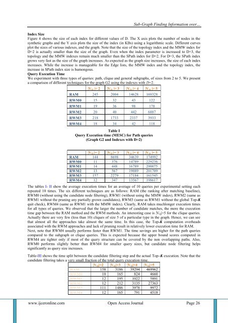
Sub-Graph Finding Information over…
Index Size
Figure 4 shows the size of each index for different values of D. The X axis plots the number of nodes in the
synthetic graphs and the Y axis plots the size of the index (in KBs) using a logarithmic scale. Different curves
plot the sizes of various indexes, and the graph. Note that the size of the topology index and the MMW index for
D=2 is actually smaller than the size of the graph. Even when the index parameter is increased to D=3, the
topology and the MMW indexes remain much smaller than the SPath index for D=2. For D=3, the SPath index
grows very fast as the size of the graph increases. As expected as the graph size increases, the size of each index
increases. While the increase is manageable for the Edge lists, the MMW index and the topology index, the
increase in SPath index size is humongous.
Query Execution Time
We experiment with three types of queries: path, clique and general subgraphs, of sizes from 2 to 5. We present
a comparison of different techniques for the graph G2 using the indexes with D=2.
|V Q |= 2 |V Q |= 3 |V Q |= 4 |V Q |= 5
RAM 245 2004 14628 169328
RWM0 15 32 43 122
RWM1 19 36 98 178
RWM2 20 40 442 6887
RWM3 218 1733 2337 3933
RWM4 18 34 42 118
Table I
Query Execution time (MESC) for Path queries
(Graph G2 and Indexes with D=2)
|V Q |= 2 |V Q |= 3 |V Q |= 4 |V Q |= 5
RAM 144 8698 34639 174992
RWM0 11 376 14789 229236
RWM1 14 448 16789 200075
RWM2 13 567 19089 201709
RWM3 157 2279 17184 161545
RWM4 12 347 13567 198617
The tables I- II show the average execution times for an average of 10 queries per experimental setting each
repeated 10 times. The six different techniques are as follows: RAM (the ranking after matching baseline),
RWM0 (without using the candidate node filtering), RWM1 (without using the MMW index), RWM2 (same as
RWM1 without the pruning any partially grown candidates), RWM3 (same as RWM1 without the global Top-K
quit check), RWM4 (same as RWM1 with the MMW index). Clearly, RAM takes muchlonger execution times
for all types of queries. We observed that the larger the number of candidate matches, the more the execution
time gap between the RAM method and the RWM methods. An interesting case is |V Q |=5 for the clique queries.
Actually there are very few (less than 10) cliques of size 5 of a particular type in the graph. Hence, we can see
that almost all the approaches take almost the same time. In this case, the Top-K computation overheads
associated with the RWM approaches and lack of pruning result in relatively lower execution time for RAM.
Next, note that RWM4 usually performs faster than RWM1. The time savings are higher for the path queries
compared to the subgraph or clique queries. This is expected because the upper bound scores computed in
RWM4 are tighter only if most of the query structure can be covered by the non overlapping paths. Also,
RWM0 performs slightly better than RWM4 for smaller query sizes, but candidate node filtering helps
significantly as query size increases.
Table-III shows the time split between the candidate filtering step and the actual Top–K execution. Note that the
candidate filtering takes a very small fraction of the total query execution time.
|V Q |=2 |V Q |=3 |V Q |=4 |V Q |=5
RAM 158 3186 39294 469962
RWM0 10 165 824 4660
RWM1 12 195 1022 5891
RWM2 12 212 3135 27363
RWM3 111 1486 3978 9972
RWM4 12 165 791 4518
www.ijceronline.com Open Access Journal Page 26