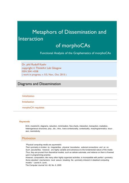
Metaphors of Dissemination and Interaction of morphoCAs

Metaphors of Dissemination and
Interaction
of morphoCAs
Functional Analysis of the Graphematics of morphoCAs
Dr. phil Rudolf Kaehr
copyright © ThinkArt Lab Glasgow
ISSN 2041-4358
( work in progress, v. 0.5, Nov., Oct. 2015 )
Diagrams and Dissemination
Initialization
Initialization
morphoCA requisites
Keywords
ECA, morphoCA, diagrams, reduction, minimization, flow charts, interaction, transaction, mediation,
heterogeneous structures, poly-, dis-, intra-, trans-contexturality, contextuality, morphogrammatics, recursion,
memristivity
Motivation
“Physical computing media are asymmetric.
Their symmetry is broken by irregularities, physical boundaries, external connections and so on.
Such peculiarities, however, are highly variable and extraneous to the fundamental nature of the media.
Thus, they are pruned from theoretical models, such as cellular automata, and reliance on them is frowned
upon in programming practice.
However, computation, like many other highly organized activities, is incompatible with perfect symmetry.
Some standard mechanisms must assure breaking the symmetry inherent in idealized computing
models.” Leonid A. Levin,
The Computer Journal Vol. 48, No. 6, 2005

2 Diagram.nb
Minimization and flow charts
It is not easy to explain how to understand the results of morphoCAs. It seems that there is a strong conflict between
the millions of visualizations, sonifications and structurations managed by the approach of claviatures and the
paradigmatic statement developed in the paper "Asymmetric Palindromes" for morphoCAs that “What you see is not
what it is”.
Instead of studying the multitude of the products of morphoCAs, another approach that is more focused on the
mechanism of the production process of morphoCAs might help to uncover the deep-structural significance of
morphogrammatic based cellular automata.
This paper offers some insights into the mechanism of production by the application of reductions (minimizations) of
the functional interpretations of the morphoCA rules and by designing the network of the actions of the morphic
automata by some flow charts.
There is not yet an algorthmic approach to reduce morphic CA functions accessible. But the distinction between
reducible and non-reducible morphoCAs is well defined.
Hence, instead of considering the multi-millions of morphoCA productions, some specific flow charts of the mechanism
of production is presented to continue the studies of morphoCAs. With that a kind of reflection a kind of a metatheory
of morphoCAs is introduced.
From this meta-theoretial point of view, morphoCAs might be involved into an introspection between Kaluzhnine-
Graph-Schemata of recursivity and poly-contextural memristivity.
A further approach to study the deep-structure of the meaning of morphoCAs will be sketched in a further paper by
an analysis of their underlying poly-contextural logics.
Contexturality vs. contextuality
The term “polycontexturality” occurs frequently in sociological studies. Often as a synonyme or replacement of
‘polycentricity’ and linguistically, modal-logically or semiotically identified with ‘contextuality’.
Polycontexturality refers to a trans-classical paradigm of thinkind and writing that is not compatible with established
concepts of science, while ‘polycentricity’ and ‘contextuality’ are parts of classical logic (say, modal logic), ontology
and semiotics.
“Polycentricity is similar to the concept of polycontexturality in logic. Polycontexturality represents a manysystem
logic, in which the classical logic systems (called contextures) interplay with each other, resulting in
a complexity that is structurally different from the sum of its components (Kaehr and Mahler 1996).”
(Rajendra Singh, Towards Information Polycentricity Theory: Investigation of a Hospital Revenue Cycle,
2011)
A similar approach, chosen out of the ‘polycentricity or centextualist movement’, is proposed e.g. by Lars Qvortrup:
“The implicit idea behind the first three theses is that we are on our way into a society, which is radically
different from the so-called modern society. It has been described as “functionally differentiated” (Luhmann
1997), as “polycontextural” (Günther 1979) or as “hypercomplex” (Qvortrup 1998), emphasising that it does
not offer one single point of observation, but a number of mutually competing observation points with each
their own social context.”
Lars Qvortrup, THE AESTHETICS OF INTERFERENCE: From anthropocentrism to polycentrism and the
reflections of digital art
http://www.hotelproforma.dk/Userfiles/File/artikler/lq.pdf
It might provoke some progress if the distinctions proposed in this paper would be applied to systems theory of intra-,
inter- and trans-contexturally mediated complex dis-contextural constellations and dynamics.
http : // memristors.memristics.com Morphospheres Asymmetric %20 Palindromes.html
http : // scholarworks.gsu.edu / cgi / viewcontent.cgi ? article = 1003 & context = ceprin_diss
More entertainment with intra-, inter- and trans-disciplinarity of inter-, poly-, trans- and dis-contexturality at: “Modular
Bolognese, Paradoxes of postmodern education” in: Short Studies 2008. Adventures in Diamond Strategies of
Change(s)
http : // works.bepress.com / cgi / viewcontent.cgi ? article = 1007 & context = thinkartlab
Three kinds of morphoCA diagrams

Diagram.nb 3
Three kinds of morphoCA diagrams
Three kinds of morphoCA diagrams have to be distinguished:
1. Mono-contextural diagrams (intra)
intra
The first kind is covered by the classical diagrams. These diagrams hold for classical ECAs as much as for monocontextural
morphoCAs of different topological complexity. Morphogrammatically, they are supported by the
‘classical’ morphograms of complexity 2.
2. Poly - contextural diagrams as interaction (inter, trans)
The second kind is based on a distribution of the diagram of at least 3 loci. This distribution is basic for the interactions
between otherwise autonomous automata. The internal structure of the memory/logic unit of the single
automata is intrinsically changed toward a chiastic, i.e. memristive behavior of internal and external events.
The interactional activity of the second kind of diagrams is supported by the morphograms of complexity 3.
In this field of interactional activity of complexity 3, two different modi might be distinguished:
• inter-actional with morphograms mg[5], mg[10] and mg[14], and head[{1,2,3}] -> i, i=1,2,3
• trans-contextural mg[11], mg[12] and mg[13] with head [{1,2}] -> 3.
3. Poly - contextural diagrams as mediation

4 Diagram.nb
The third kind is based on the second kind but is involving the whole structural complexion of the distributed morpho-
CAs. Only with this configuration the full graphematic character of morphoCAs enters the trans-classic game of
computation, interaction, reflection and mediation.
Mediative actions are supported by morphograms of the minimal complexity 4, represented by the morphogram
mg[15] with head[{1,2,3}]->4.
Poly - contextural basic component
inter
intra
trans
intra
Exam ples
Functions
intra : 0, 0, 0 → 0 : sys1, 1, 1 → sys1, 1, 1
trans : 0, 0, 1 → 2 : sys1, 1, 1 → sys3 || sys1 || sys3
inter : 1, 2, 1 → 0 : sys2, 1, 2 → sys1 || sys3 || sys1
med : 1, 0, 2 → 3 : sys1, 2, 3 → sys5 || sys4 || sys6
Action schemes
intra iteration scheme
t
C k-1 , C t t
k , C k+1
C k t+1 ≡ C k
t
inter / trans - action scheme
t
C i,k-1
t
, C i,k , C i,k+1
t
t
|| C j,k-1
t
, C j,k , C j,k+1
t+1
C i,k ⟶ C t+1 t+1
i,k ≡ C j,k
t
t
C k-1 , C t t
k , C k+1
t
C j,k-1
t
, C j,k , C j,k+1
t
C k t+1 ≡ C k
t
Morphograms

Diagram.nb 5
intra
R1 R2 R3 R4
■ ■ ■
- ■ -
■ ■ □
- ■ -
■ □ ■
- ■ -
■ □ □
- ■ -
R6 R7 R8 R9
■ ■ ■
- □ -
■ ■ □
- □ -
■ □ ■
- □ -
■ □ □
- □ -
trans
R11 R12 R13
■ ■ □
- ■ -
■ □ ■
- ■ -
■ □ □
- ■ -
inter
R5 R10 R14
■ □ ■
- ■ -
■ □ ■
- □ -
■ □ ■
- ■ -
mediation
R15
■ □ ■
- ■ -
The compound morphogram ruleDM[{1, 3, 4, 11, 15}] inscribes the deep-structure of the mediation of intra- and intercontextural
actions.
■ ■ ■
- ■ -
■ □ ■
- ■ -
■ □ □
- ■ -
■ ■ □
- ■ -
■ □ ■
- ■ -
Poly-contextural logic
Quite obviously, intra-contextural morphograms are representing the deep-structure of junctional mono- and polycontextural
operators.
As a first remark, inter- and trans-contextural morphograms are representing the deep-structures of transjunctional
poly-contextural operators.
Morphogram mg[15] represents the full differentiations of the interplay of inter- and trans-contextural poly-contextural
operators.
The proof-theoretical metaphor of polycontextural interplays is not anymore just a ‘tree’ but a ‘forrest of colored trees’.
Example: ternary 3-contextural transjunctions of ruleDCM[{1, 2, 12, 13, 5}]
{0, 0, 0} → 0, {0, 0, 1} → 0 : dis - junctions in syst1,
{0, 0, 2} → 0 : junction in syst3, "0⋀(0⋁2)≡ 0",
{2, 2, 0} → 2 : junction in syst3, "2⋀(2⋁0)≡ 2",
{0, 1, 0} → 2, {1, 0, 0} → 2 : trans - junctions from syst1 to sys2 || sys3,
{1, 2, 1} → 0 : trans - junctions from syst2 to sys1 || sys3
{0, 2, 2} → 1, {2, 0, 0} → 1 : trans - junctions from syst3 to sys1 || sys2,
{0, 1, 2} → 0, {2, 1, 0} → 2 : trans - junctions from syst1, 3, 2 to sys1 || sys3
1. Mono-contextural diagrams: ECA and morphoCA (m,2,n)

6 Diagram.nb
1. Mono-contextural diagrams: ECA and morphoCA (m,2,n)
Diagram of the ECA scheme
K. Salman’s paper “Elementary Cellular Automata (ECA) Research platform” gives an elaborated definition and
explanation of the concept of ECAs.
For the purpose of an introduction of morphoCAs it suffice to connect to some of its terms and constructions.
“For ease of illustration we let the CA evolve according to one uniform neighborhood transition function and
fixed radius which is a local function (rule) 3 0 : 4 2 r+1 ⟶ 4 where the CA evolves after a certain number of
time steps T.
In this case we have a total of 5 2 r+1 distinct rules. It follows that a 1 - D CA is a linear lattice or register of 6∈
N memory cells. Each cell is represented by C k
t , where 9 = [1: 6], 6∈ N and : = [1: ;], ;∈ Z that
describes the content of memory location at evolution time step t..” (K. Salman)
Figure 5, Detailed Structure of a typical Cellular Automaton Cell for rule 30.
http : // www.cyberjournals.com/Papers/Jun2013/02. pdf
Diagram of the CA rule in respect of input and output cells in time t to t+1
move right
http : // www.slideshare.net / ijcsit / 5413 ijcsit03
Description of the mechanism of the CA calculation
The object D k of C k
t+1
of Fig. 5 is a result of the calculation of the logical unit U, i.e. Transition Rule Logic, in relation
t t
to its inputs C k+1 and C k-1 , but it is also at the same time the initial value, Q k , in the Memory Cell, of a new calculation
of a next step of the CA.
This new calculation might happen intra-contexturally as a mapping from Q k as Q i to the logic unit U i or transcontexturally
as a mapping from Q k as Q i to the new object D k of D k
i+1
in CA 2.1 where it becomes the new value of
Q k i+1 for a calculation in CA 2.2 .
The presumption of the classical model of ECAs is certainly that all components are from the same contexture, and
having the same clock.
Mono-contextural CAs are homogeneous structures.

Diagram.nb 7
Classical Cellular Automata. Homogeneous Structures
By V. Z. Aladjev
intra iteration scheme
[Ct k-1 , C t k , Ct
k+1
C k t+1 ≡ C k
t
Ct k-1 , C t k , Ct
k+1
C k t+1
≡ C k
t
inter / trans interaction scheme
Ct
i,k-1
, Ct
i,k , Ct
i,k+1
] || Ct
j,k-1
, Ct
j,k , Ct
j,k+1
Ct+1 i,k ⟺ intertrans
C t+1 j,k ≡ Ct
j,k
intra
Ct
j,k-1
, Ct
j,k , Ct
j,k+1
inter / trans interaction network scheme
Ct
i,k-1
, Ct
i,k , Ct
i,k+1
] || Ct
j,k-1
, Ct
j,k , Ct
j,k+1 || [Ct
h,k-1 , Ct
h,k , C h,k+1
t
]
⟺
C t+1 i,k ≡ Ct
i,k
⟺ intertrans
C t+1 j,k ≡ Ct j,k ⟺ intertrans
C t+1 h,k ≡ Ct
h,k
⟺
intra
Ct
i,k-1 , Ct i,k ,
Ct
i,k+1
|| Ct
j,k-1
, Ct
j,k , Ct
j,k+1
|| Ct
h,k-1
, Ct
h,k , Ct
h,k+1
Diagram of the sub-rule definition of ECAs
A sub-rule implementation of the ECA rules might augment its computational efficiency and reduce numeric complexity
for programmable hybrid ECA compositions.
As it is well known, CAs are understood as parallel computing concepts and devices.
There is no doubt that the sketched sub-rule appoach can be concretized and implemented as a ‘hybrid’ ECA on a
hardware board like Spartan-6 FPGA Connectivity Kit or similar.
(http://www.xilinx.com/products/boards-and-kits.html)
A further step in augmenting the granularity of CAs might be achieved with the sub-rule approach for ECA rules.
Each ECA rule is defined in a sub-rule oriented approach as a composition of sub-rules. Thus all compatible subrules
can be applied in parallel to realize a single ECA rule.
Also the sub-rule approach is defining the ECA rules is not yet showing the flow chart of the interactions of the subrules
to build the ECA rule.
ECA-rule = [eca1, eca2, ..., eca8]
Example: ECA rule 210

8 Diagram.nb
t
C k-1 , C t k ,
t
C k+1
t+1
C k
: intra
ruleECA[{6, 7, 3, 9, 10, 12, 13, 15}]
{{0, 0, 0} → 1,
{0, 0, 1} → 1,
{0, 1, 0} → 0,
{0, 1, 1} → 1,
{1, 0, 0} → 0,
{1, 0, 1} → 0,
{1, 1, 0} → 1,
{1, 1, 1} → 0}
210
FromDigits[{1, 1, 0, 1, 0, 0, 1, 0}, 2]
Hence the ECA rule 210 is represented by the tuple (6,7,3,9,10,12,13,15) of ECA sub-rules.
Flow chart of the parallel realization of the 8 sub - rules of an ECA.
“If in a CA the same rule applies to all cells, then the CA is called a uniform CA; otherwise the CA is called a hybrid
CA (Fig. 1).”
Theory and Applications of Cellular Automata in Cryptography
S.Nandi, B.K.Kar and P.Pal Chaudhuri
ECA sub-rule manipulators
The method of sub-rules for ECAs is an abstraction and parametrization of the components of the rule schemes that
allows a micro-anlysis of the ECAs. The ECA sub-rule manipulator manages all ECA rules of a 1D ECA. The subrule
manipulators enables a micro-analysis of the behavior of all 2 8 ECA rules.
Each 1-D ECA rule number has a sub-rule number representation. There are just 8 disjunct pairs of sub-rules to
define a 1D ECA rule.
The results are visualized below. The combination of the 8 sub-rules covers all the 256 well known ECA rules.

Diagram.nb 9
k 1 6
l 2 7
m 3 8
n 4 9
o 5 10
p 11 12
q 13 14
r 15 16
steps 44
Mono-contextural ruleDCKF (5,2,3)
a 1111 1112
b 1121 1122
c 1211 1212
d 2111 2112
e 1221 1222
f 2121 2122
g 2212 2211
h 2221 2222
steps 22
mesh
Reduction (trivial)
ruleDCKF[{1111, 1122, 1211, 2112, 1221, 2121, 2211, 2222}]

10 Diagram.nb
intra
{1, 1, 1, 1} → 1, {0, 0, 0, 0} → 0, : Sys1
{1, 1, 1, 0} → 0, {0, 0, 0, 1} → 1,
{1, 1, 0, 1} → 1, {0, 0, 1, 0} → 0,
{1, 0, 1, 1} → 0, {0, 1, 0, 0} → 1,
{1, 1, 0, 0} → 1, {0, 0, 1, 1} → 0,
{1, 0, 1, 0} → 1, {0, 1, 0, 1} → 0,
{1, 0, 0, 1} → 1, {0, 1, 1, 0} → 0,
{1, 0, 0, 0} → 0, {0, 1, 1, 1} → 1
Random
Scheme: (r1, r2, r3, r4) ⟹ r5, r i = {0, 1}
r3
r5
r1r2
ruleDCKF
r4
2. Poly-contextural diagrams with interactions
General approach
Internal structure of the memory unit of the second kind
Following for example K. Salman’s classical modelling approach in “Elementary Cellular Automata (ECA) Research
platform“ a more explicit modelling of the mechanism of morphoCAs might be achieved.
A first crucial difference to the classical concept is the fact that the memory unit is not just passively receiving (D) and
sending data (Q) but is also actively deciding to which system of its computational environment they belong and if the
data remain in its domain or not. If not, the activity of the memory unit is deciding where that data belong and sends it
to the evoked computational unit of the complexion.
In terms of actors, the memory unit is receiving, sending and deciding about the contextures of data. Classical
memory actions are strictly intra-contextural. This holds in the same sense for multi-processor systems too. They are
acting strictly intra-contexturally, keeping their distributed data together.
Hence, the logic devices in the modified diagram, Fig. 5b, have two function towards its memory units:
1. a decision operation over the logical operations, i.e. to decide if an operation stays inside the contexture or if it
leaves trans-contexturally the contexture for another contexture on another layer of the complex poly-layered
morphoCA system.
2. the intra-contextural function of producing the junctional values for the corresponding intra-contextural memory in
the sense of ordinary logical functions, like NAND or NOR.

Diagram.nb 11
Hence, the logic devices in the modified diagram, Fig. 5b, have two function towards its memory units:
1. a decision operation over the logical operations, i.e. to decide if an operation stays inside the contexture or if it
leaves trans-contexturally the contexture for another contexture on another layer of the complex poly-layered
morphoCA system.
2. the intra-contextural function of producing the junctional values for the corresponding intra-contextural memory in
the sense of ordinary logical functions, like NAND or NOR.
The object D k of the CA diagram receives a value from the logic unit and it delivers it to Q as Q k for the new calculation
with c k of the logical unit in time t + 1.
Secondly, Q receives the value from D as a value, not for Q 1.1 in CA 1 but for Q 2.1 of the neighbor layer CA 2 . This new
value is memorized in the neighbor CA 2 as the new positive value for calculation in CA 2 , hence it is placed in
CA 2.1 and not as a genuine value of CA 2 as CA 2.2 .
The result of the application of the rule in all 3 sub-systems is delivered with the multi-layered system as a whole, i.e.
with morphoCA (3,3) and its rules R (3,3) .
Obviously, the whole automaton with its different layers has to be designed in the epistemological mode of the ‘asabstraction’,
i.e. as “A as B is C” and not in the mode of identity with “A is A”.
The modified diagram is introducing an environment to the original mono-contextural CA diagram that implies
the possibility of interactions. The environment of a CA system is the primary condition for a possible selfreflection
of the complex system of different and interacting CAs.
The logic behind this construction was first introduced by Gotthard Gunther’s “Cognition and Volition” (1970)
which gives a profound explanation of the new concept of the ‘proemial relation’.
Modified diagram Fig. 5b
Memristive properties of the memory/logic unit
Why and how is the behavior of the memory units of morphoCAs of second-order and memristive and not just
defined as first-order actions of storage and transformations? The main strategy of the whole maneuver is to avoid
‘information processing’. Interaction is prior to information exchange.
It could be said: morphoCAs without memristivity are reducible without loss to classical CAs.
internal :
external :
D k 1.1 ⟹
1.1 2.2
Q k > k
⇵ ⇵
U 1.1 → D k 1.1 ⟹
1.1
Q k > 2.2 k ⟶ 4 2.2 k : C 2.1 k → U 2.2
⇕ ⇵
Q k 1.2 ⟹ Q k
2.1
Q k 1.2 ⟹ Q k
2.1
The diagram below, Fig. 1, shows again the chiastic interaction between operators (M) and operands ‘σ’ distributed
over different loci of the kenomic matrix.
“M as σ” is obviously not the so called self-reference of “M is σ”.
Χ (M, σ) =
M 1.1 ⟹σ 2.1 M 2.2 ⟹σ 1.2
x
σ 2.2 ⟹M 1.2 σ 1.1 ⟹M 2.1
http : //
memristors.memristics.com / semi - Thue / Notes %20 on %20 semi - Thue %20 systems.html
Fig . 1 Chiasm (M, σ)

12 Diagram.nb
Explanation of Fig. 1
"The wording here is not only
" types becomes terms and terms becomes types " but
“ a type as a term becomes a term " and, at the same time,
"a type as type remains a type".
Thus, "a type as a term becomes a term and as a type it remains a type".
And the same round for terms.
Full wording for a chiasm between terms and types over two loci
Explicitly, first the green round,
"A type σ 1.1 as a term M 2.1 becomes a term M 2.1
and as a type σ 1.1 it remains a type σ 1.1 for a term M 1.1 ".
And,
"A type σ 2.2 as a term M 1.2 becomes a term M 1.2
and as a type σ 2.2 it remains a type σ 2.2 for a term M 2.2 ".
And simultaneously, mediated,
the second round in red, the same for terms:
"A term M 1.1 as a type σ 2.1 becomes a type σ 2.1
and as a term M 1.1 it remains a term M 1.1 for a type σ 1.1 ".
And,
"A term M 2.2 as a type σ 1.2 becomes a type σ 1.2
and as a term M 2.2 it remains a term M 2.2 for a type σ 2.2 ".
And finally, between terms M 1.1 and M 2.2 and types σ 1.1 and σ 2.2 ,
a categorial coincidence is realized.
While between terms and types a morphism (order relation) exists.
Fig . 2 Complete interactional scheme

Diagram.nb 13
interaction scheme
t
C i,k-1
t
, C i,k , C i,k+1
t
t
|| C j,k-1
t
, C j,k , C j,k+1
t
t+1
C i,k
⟶
C t+1 t
j,k ≡ C j,k
t
C j,k-1
t
, C j,k , C j,k+1
t
Hence, this kind of memory is a complexion of ‘memory’ and ‘logic’ as it is supposed for memristive behavior.
There are four basic components plus the clock in the interaction paradigm of morphoCAs.
Calculation :
sendreceive,
acceptreject
in generalized time
In contrast to the classical CA with its send/receive properties, there are four basic components plus the clock in the
paradigm of morphoCAs. The sens/receive or read/write mechanism is augmented in morphoCAs by a decisionmaking
(trans-logical) component of accept/reject in regard of the sub-system property.
The contrast to Konrad Zuse's conception of calculation is obvious :
“Rechnen heisst : Aus gegebenen Angaben nach einer Vorschrift neue Angaben bilden.” (Konrad Zuse)
The discontexturaliy of morphoCAs is certainly also not in hamony with Karl Hewitt’s monolithic actor approach to
computation.
A systematic deconstruction has obviously to deconstruct all 4+1 components of the diagram.
The very first deconstruction happens by parametrizing the inputs. Each input/output, i.e. send/receive action might
belong to a different contexture. Hence, the very first task of the automaton is to handle such profound diversity. This
job is obsolete for classical CAs because all data are from/in the same contexture.
This contextural embodiment of the fourth term, C k
t+1 , explains why the term is not just an extensional result of a
mapping but is structurally depending on the conceptual ‘history’ of the 3 previous actions.
This understanding of the morphoCA rules relates back to the concept of the ϵ/ν-structure of morphic objects and
actions within the concept of the proposed memristive automata.
http : // www.thinkartlab.com / pkl / media / SKIZZE - 0.9
http : // works.bepress.com / thinkartlab / 20 /
http : // transhumanism.memristics.com / Diagrammatik.ppt.htm
.5 - medium.pdf
From memristive flip-flop to memristive interactions
Finite state machines and morphoCAs
“A Cellular Automaton (CA) is an infinite, regular lattice of simple finite state machines that change their states
synchronously, according to a local update rule that specifies the new state of each cell based on the old states
of its neighbors.” (Kari)
http://users.utu.fi/jkari/ca/CAintro.pdf
“Furthermore, since the ECA is actually a finite state machine then the present state of the neighborhood
C k-1 , C t t t t+1
t
k , C k+1 of cell C k at time step t and the next state C k at time step t + 1, can be analyzed
by the state transition table and the state diagram depicted in figure 4.” (K. Salman)

14 Diagram.nb
“Furthermore, since the ECA is actually a finite state machine then the present state of the neighborhood
C k-1 , C t t t t+1
t
k , C k+1 of cell C k at time step t and the next state C k at time step t + 1, can be analyzed
by the state transition table and the state diagram depicted in figure 4.” (K. Salman)
Figure 4, state machine analysis of Rule 30
http : // www.slideshare.net / ijcsit / 5413 ijcsit03
ECA Rule 30
FromDigits[{0, 0, 0, 1, 1, 1, 1, 0}, 2]
30
FromDigits[kAryFromRuleTable[
ruleECA[{1, 2, 3, 9, 5, 11, 13, 15}]], 2]
30
ruleECA[{1, 2, 3, 9, 5, 11, 13, 15}] = rule30
rule30 111 110 101 100 011 010 001 000
1 - - - (5) : 1 (9) : 1 (3) : 1 (2) : 1 -
0 (15) : 0 (13) : 0 (11) : 0 - - - - (1) : 0
http : // memristors.memristics.com / MorphoFSM / Finite
%20 State %20 Machines %20 and %20 Morphogrammatics.html
System of elementary kenomic cellular automata rules in trito-difference form
R1 R2 R3 R4
R5
■ ■ ■
- ■ -
■ ■ □
- ■ -
■ □ ■
- ■ -
■ □ □
- ■ -
■ □ ■
- ■ -
R6 R7 R8 R9
R10
■ ■ ■
- □ -
■ ■ □
- □ -
■ □ ■
- □ -
■ □ □
- □ -
■ □ ■
- □ -
R11 R12 R13 R14 R15
■ ■ □
- ■ -
■ □ ■
- ■ -
■ □ □
- ■ -
■ □ ■
- ■ -
■ □ ■
- ■ -

Diagram.nb 15
e1 e2 e4
- e3 e5
R1 - e6
e1 e2 v4
- e3 v5
R6 - v6
e1 v2 v4
- v3 v5
R11 - v6
e1 v2 e4
- v3 e5
R2 - v6
e1 v2 v4
- v3 v5
R7 - e6
v1 e2 v4
- v3 v5
R12 - v6
v1 e2 e4
- v3 v5
R3 - e6
v1 v2 v4
- e3 e5
R8 - v6
v1 v2 e4
- v3 v5
R13 - v6
v1 v2 e4
- e3 v5
R4 - v6
v1 v2 v4
- e3 e5
R9 - e6
v1 v2 v4
- v3 e5
R14 - v6
v1 v2 v4
- e3 v5
R5 - v6
v1 v2 v4
- v3 v5
R10 - e6
v1 v2 v4
- v3 v5
R15 - v6
Interpretation
Difference scheme
The difference scheme is a scheme of differences, and not just a relational mapping from C 3 to C.
Also an evolution from [Ct k-1 , C kt , Ct
k+1 ] to Ct+1 k is defined by all previous elements of time t of the specified
CA rule there is no concrete differentiation between the new state of Ct+1 k and the previous states defined.
Hence, the new state C k
t+1 of a classical CA might incorporate any arbitrary value from a pre-given set of values
and is not retro-recursive characterized by the differences of the previous constellation it depends.
C k-1 , C t k ,
t
C k+1
t+1
C k
⟹
t
C k-1 , C t t
k , C k+1
t+1
C k
⟹
d1 d2 d4
- d3 d5
- - d6
, with d = {ϵ, ν}, ϵ = equal, ν = non-equal
FSA Example
t
d1 = diff ( C k-1 , C t k ),
t t
d2 = diff ( C k-1 , C k+1 ),
d3 = diff ( C t t
k , C k+1 ),
t
d4 = diff ( C k-1 , C t+1 k ),
t
d5 = diff ( C k+1 , C t+1 k ),
d6 = diff ( C t k , C t+1 k ).
FSA(aabc)
MorphoFSA[aabc]

16 Diagram.nb
http : // memristors.memristics.com / CA -
Overview / Short - %20 Overview %20 of %20 Cellular %20 Automata.pdf
Monomorphic prolongation
First aspect: iteration
Given a morphogram MG, which is always a localized pattern in a kenomic matrix, a prolongation (successor,
evolution) of the morphogram is achieved with the successor operator s i . To each prolongation a further prolongation
is defined by the iterated application of the operator s i .
The morphogrammatic succession MG ⟶ s i
MG is founded by its model gm ⟶ h j
gm and the morphism f, guaranteeing
the commutativity of the construction.
As a third rule, the iterability of the successor operation is arbitrary, which is characterised by the commutativity of
the diagram. Hence, the conditions for a (retrograde) recursive formalisation are given.
Second aspect: anti-dromicity
Each prolongation is realized simultaneously by an iterative progression and an antidromic retro-gression. That is,
the operation of prolongation of a morphogram is defined retro-grade by the possibilities given by the encountered
morphogram. A concrete prolongation is selecting out of those possibilities its specific successions. All successions
are to be considered as being realized at once.
Third aspect: simultaneity and interchangeability
This simultaneity of different successions defines the range of the prolongation. This definition of morphogrammatic
prolongation is not requiring an alphabet and a selection of a sign out of the alphabet. Hence, the concept of morphogrammatic
prolongation is defined by the two aspects of iteration and antidromic retro-gradeness of the successor
operation. The simultaneity of the prolongations is modeled by the interchangeability of its actions.
Fourth aspect: diamond characterization of antidromicity
Both aspects together, repeatability and antidromicity with its simultaneous and interchangeable realizations, are
covered by the diamond-theoretic concept of combination of operations and morphisms, i.e. composition and
saltisition, between morphogramatic prolongations.
The philosophical status of morphoCAs has yet to be determined.“What’s after digitalism?” might give a hint.
https : // www.academia.edu / 1 873 531 / Digital_Philosophy._Formal
_Ontology _and _Knowledge _Representation _in _Cellular _Automata
Internal structure of the morphogrammatic transition rule
Recall definitions: classical transition rule
"Rigid computations have another node parameter: location or cell. Combined with time, it designates the
event uniquely. Locations have structure or proximity edges between them. They (or their short chains)
indicate all neighbors of a node to which pointers may be directed.
“CA are a parallel rigid model. Its sequential restriction is the Turing Machine (TM). The configuration of CA
is a (possibly multi-dimensional) grid with a fixed (independent of the grid size) number of states to label
the events. The states include, among other values, pointers to the grid neighbors. At each step of the
computation, the state of each cell can change as prescribed by a transition function of the previous states
of the cell and its pointed-to neighbors. The initial state of the cells is the input for the CA. All subsequent
states are determined by the transition function (also called program)." Leonid A. Levin. Fundamentals of
Computing.

“CA are a parallel rigid model. Its sequential restriction is the Turing Machine (TM). The configuration of CA
is a (possibly multi-dimensional) grid with a fixed (independent of the grid size) number of states to label
the events. The states include, among other values, pointers to the grid neighbors. At each step of the
Diagram.nb 17
computation, the state of each cell can change as prescribed by a transition function of the previous states
of the cell and its pointed-to neighbors. The initial state of the cells is the input for the CA. All subsequent
states are determined by the transition function (also called program)." Leonid A. Levin. Fundamentals of
Computing.
http://www.cs.bu.edu/fac/lnd/toc/z/z.html
Morphogrammatic transition rule
http : // memristors.memristics.com / Memristive %20
Cellular %20 Automata / Memristive %20 Cellular %20 Automata.html
General scheme
rule set, start string
string pos = (Nr., l)
ReLabel
ReLabel (string)
↙ ↘ NextGen
NextGen (ReLabel (string))
↘ ↓ ↙ ∈ rule - set?
〈yes; no〉
apply rule
result
Example
rule set = {1, 7, 8, 4}, start string
[bcb] : string at pos (Nr., l)
ReLabel
[aba]
↙ ↘ NextGen
[abaa][abab][abac]
↘ ↓ ↙ [abaa] ∈ rule - set?
〈yes; no〉
apply : [abaa] rule7
result = [a]
NextGen is in this morphoCA context a retrograde recursive action and not to be confued by a classical recursion.
What makes the difference?
1. retro - grade recursivity
2. irreducible heterogeneity
3. interactivity and reflectionality
Morphogrammatic example
evol i (MG) :
∀ i ∈ (mg (MG)), 1 ≤ i ≤ mg (MG) + 1
second
selection
retrogression
first
choice
([mg 1 ... mg i ... mg n ] ⟶ [mg 1 ... mg i .. mg n ]) ⟶ [mg 1 ... mg i ... mg n mg n+1 ]
first
choice
⟶
progression
second
selection
http : // memristors.memristics.com / MorphoReflection / Morphogrammatics
%20 of %20 Reflection.html
Flow charts for morphoCAs
Full mediation of input

18 Diagram.nb
Basic scheme : Explanation for morphoCA (3,3)
Clock (3,3)
= synch Clock 1.1 , Clock 2.2 , Clock 3.3
Calculation (3,3) = mediation TRL1 .1, TRL2 .2, TRL3 .3 :
TRL 1 ∐ 1.2,0 TRL 2 ∐ 1.2,3 TRL 3 =
TRL 1 -
- TRL 3
TRL 2 -
intra (3,3) = ( TRL1 .1 (Ct1k, Ct1k + 1, Ct1k - 1)
∐
TRL2 .2 (Ct2k, Ct2k + 1, Ct2k - 1))
∐
TRL3 .3 ((Ct3k, Ct3k + 1, Ct3k - 1)
ENV (3,3) = [ ENV 1 ∐ ENV 2 ] ∐ ENV 3 :
Ct1k + 1 ∐ Ct3k + 1
Ct2k - 1 ∐ Ct2k + 1
Ct3k - 1 ∐ Ct3k - 1
ENV 1 ∐ 1.2,0 ENV 2 ∐ 1.2,3 ENV 3 =
ENV 1 -
- ENV 3
ENV 2 -
Arrows
directed arrows : input/output arrows,
open headed arrows : inter - and trans - action, mediation arrows
Explanation for morphoCA (4,4)

Diagram.nb 19
morphoCA (4,4) =
CA1 E E
- CA3 E
CA2 E CA6
E CA5 E
CA4 E E
::
Full interaction and mediation table for morphoCA (3,3)
S11 S11 S21, 31
S22 S22 S12, 32
S33 S33 S13, 23
S1 D11 - Q11 Q12 - D21, Q13 - D31
S2 D22 - Q22 Q21 - D12, Q23 - D32
S3 D33 - Q33 Q13 - D31, Q23 - D32
morphoCA (3,3) :
CA 1 2 3
1 CA 1.1 CA 2.1 CA 3.1
2 CA 1.2 CA 2.2 CA 3.2
3 CA 1.3 CA 2.3 CA 3.3
Discontexturality of distributed CAs

20 Diagram.nb
Poly-layered grid structure
... C1tk + 1 C1tk C1tk - 1 ...
... C2tk + 1 C2tk C2tk - 1 ...
... C3tk + 1 C3tk C3tk - 1 ...
⟹
... C1t + 1 k + 1 C1t + 1 k C1t + 1 k - 1 ...
... C2t + 1 k + 1 C2t + 1 k C2t + 1 k - 1 ...
... C3t + 1 k + 1 C3t + 1 k C3t + 1 k - 1 ...
An interpretation of the discontexturality diagram shows that the grid structure of distributed CAs of the morphoCAs
are in fact not 1-D CAs but disseminated 1-D CAs. It also shows that disseminated CAs are not necessarily 2- or 3-
dimensional or higher. What we see as a linear 1-D grid by the visualization of morphoCA actions is in fact a
composition of different parallel 1-D grids projected onto an 1-D grid of an uninterpteted output.
Hence, in functional terms, there is no mapping from {0, 1, 2, 3} 3 -> {0,1,2,3} but a composition of partial sub-maps.
Nevertheless, poly-layered grids are not multi-layered, because the layers of a multi-layered system are unified
under the umbrella of First-Order Logic with Modal logic and General Ontology (Upper Ontology). While discontexturality
implies an interplay of a multitude of irreducibly different logics, each containing their inter- and translogical
operators, additionally to the full set of intra-logicial operators too.
Multi-layerd systems are logically defined by the basic intra-logical operations only. Poly-layerd systems are
involved in an interplay of dis-contextural operations of inter- and trans-contextural actions.
This discontextural approach obviously is in strict conflict with Proposition1 of category theory and its unique
universe U:
If x ∈ U and y ⊆ x, then y ∈ U.
As usual in such fundamental situation, the proposition is circular. It presumes the uniqueness of its logical universe
to work for a definition of its unique category-theoretical universe which is taken as the base for the definition of
First-Order Logic and its unique universe of terms.
“Polycontexturality alone is not enough to realize the interwoven dynamics a new world-view is desperate
for. Gotthard Gunther introduced his proemial relationship to dynamize his contextures, albeit still restricted
to a uni-directional movement.The concept of metamorphosis as part of the diamond strategies, based on
polycontexturality and disseminated over the kenomic matrix, is a further step to realize a radical paradigm
change in our way of thinking and designing futures.”
http : // memristors.memristics.com/Polyverses/Polyverses.html
The projection marks the difference of the deep-structure and the surface structure of the productions of
morphoCAs.
It makes it clear, again, that “What you see is not what it is”. Hence, any ontologizing will fail.

Diagram.nb 21
yellow C1t + 1 k - C3tk - 1 -
red - - - C4t + 1 k
blue - C2t + 1 k - -
green - - - -
projection ⟹ C1t + 1 k C2t + 1 k C3tk - 1 C4t + 1 k
The difference between multi-layered and poly-layered systems got a conceptual sketch with the paper:
Memristics: Dynamics of Crossbar Systems
Strategies for simplified polycontextural crossbar constructions for memristive computation
“Interchangeability is part of a new axiomatics of poly-categorical diamond systems still to be developed.
Interchangeability is defined intra-contextural for composition and yuxtaposition, and trans-contextural for
interactions, like mediation, replication, iteration and transposition.”
http://www.thinkartlab.com/Memristics/Poly-Crossbars/Poly-Crossbars.pdf
Claviatures for morphoCAs
Claviature: ruleDM
k 1 6
l 2 7 11
m 3 8 12
n 4 9 13
o 5 10 14 15
steps 11

22 Diagram.nb
Claviature: Random ruleDM
k 1 6
l 2 7 11
m 3 8 12
n 4 9 13
o 5 10 14 15
steps 44

Diagram.nb 23
Claviature: ruleDCKV
a 1111 1112
b 1121 1122 1123
c 1211 1212 1213
d 1221 1222 1223
e 2121 2122 2123
f 2211 2212 2213
g 2221 2222 2223
h 2111 2112 2113
i 2131 2132 2133 2130
j 1231 1232 1233 1230
k 2231 2232 2233 2230
l 2311 2312 2313 2310
m 2321 2322 2323 2320
n 2331 2332 2333 2330
o 2301 2302 2303 2300
steps 9
mesh
save
Analysis of ruleDM[{1,11,3,9,x}]
ruleDM[{1, 11, 3, 9, 5}]
reduced ruleDM[{1, 11, 3, 9, x}]
Subrules
Subsystems
ruleDM[1] : {0, 0, 0} → 0, S1, 3 : yellow
ruleDM[3] : {0, 1, 0} → 0, S1
ruleDM[9] : {1, 0, 0} → 0, S1
ruleDM[3] : {0, 2, 0} → 0, S3
ruleDM[9] : {2, 0, 0} → 0, S3
ruleDM[11] : {0, 0, 1} → 2, S1 → S2, 3 : blue
ruleDM[11] : {0, 0, 2} → 1, S3 → S1, 2 : red

24 Diagram.nb
ruleDM[{1, 11, 3, 9, x}]
x / yz 00 10 20 01 02
0 [1] : 0 1,3 [8] : 0 1 [8] : 0 3 [11] : 2 2,3 [11] : 1 1,2
1 [9] : 0 1 - - - -
2 [9] : 0 3 - - - -
Distribution density
0 / 5 1 / 1 2 / 1
000
010
100
200
020
002 001
Flow chart for ruleDM[{1,11,3,9,x}]
Labeled interaction diagram for ruleDM[{1, 11, 3, 9, x}]
Explicit transition system table for ruleDM[{1,11,3,9,x}]
TRL1 .1 || TRL3 .3
{0, 0, 0} -> 0
: D1 .1 → Q1 .1 → TRL1 .1 || D3 .3 → Q3 .3 → TRL3. 3
TRL1 .1
{0, 1, 0} -> 0,

Diagram.nb 25
{0, 1, 0} -> 0,
{1, 0, 0} -> 0
: D1 .1 → Q1 .1 → TRL1 .1
TRL3 .3
{0, 2, 0} → 0,
{2, 0, 0} → 0
: D3 .3 → Q3 .3 → TRL3 .3
TLR2 .2 || TLR3 .3
{0, 0, 1} → 2
: Q1 .2 → Q3 .2 → TLR3 .3 || Q1 .2 -> Q2 .1 → TLR22
TLR1 .1 || TLR2 .2
{0, 0, 2} → 1
: Q3 .1 → Q1 .3 → TLR1 .1 || Q3 .2 -> Q2 .1 → Q2 .2 → TLR22
Simplified diagram
Example: ruleDM[{1, 11, 3, 9, 15}] step-wise realization
k 1 6
l 2 7 11
m 3 8 12
n 4 9 13
o 5 10 14 15
cell
initial
start (init) : yellow, red

26 Diagram.nb
,
step 37 : {0, 0, 0} → 0, {0, 1, 0} → 0, {1, 0, 0} → 0 :
TRL1 .1 || TRL3 .3
{0, 0, 0} -> 0
: D1 .1 → Q1 .1 → TRL1 .1 || D3 .3 → Q3 .3 → TRL3 .3
TRL1 .1
{0, 1, 0} -> 0, : D1 .1 → Q1 .1 → TRL1 .1
{1, 0, 0} -> 0
Start of the morphoCA with init {{1}, 0} producing the entry “red” with an environment “yellow” with the properties
defined at step 37 by the rules:
{0,0,0}→0 of sys1||sys3 and {0,1,0}→0, {1,0,0}→0 of sys1.
construction: blue, yellow, red, yellow
step 44 : {0, 0, 1} → 2 :
TLR2 .2 || TLR3 .3
{0, 0, 1} → 2
Q1 .2 → Q3 .2 → TLR3 .3 || Q1 .2 -> Q2 .1 → TLR22
At step 44, the memory decides that the received value “2” doesn’t belong to its range, i.e. the system 1, defined by
the values {0,1}.
The value “2” of system 3 defines a new start at the system 3 with the properties of {0,0,2}→1, {0,2,0}→0, {2,0,0}→0.
step 66 : {0, 0, 2} → 1 :
TLR2 .2 || TLR3 .3
{0, 0, 1} → 2
Q1 .2 → Q3 .2 → TLR3 .3 || Q1 .2 -> Q2 .1 → TLR22
TRL3 .3
{0, 2, 0} → 0, : D3 .3 → Q3 .3 → TRL3 .3
{2, 0, 0} → 0
Again, at the step 66, the decider of the memory unit of system 3 decides that the value “1” doesn’t belong to its
range, i.e. the system 3, defined by the values {0,2}.
The value “1” of memory 3 defines a continuation in the system 1 with the background properties of {0,2,0}→0,
{2,0,0}→0.
The background is symbolized numerically by 0, i.e. yellow. But “0” belongs to 2 different sub-systems defined by {0,
1} and {0, 3}.
What counts is not just the value in a system but its contextual relation or difference to other values. Hence the
presupposed rule: {0,0,0} -> 0, holds in general but its significance depend on its context.
iteration of construction

Diagram.nb 27
step 88 : {0, 0, 1} → 2 :
TLR2 .2 || TLR3 .3
{0, 0, 1} → 2
Q1 .2 → Q3 .2 → TLR3 .3 || Q1 .2 -> Q2 .1 → TLR22
At step 88, the memory decides that the received value “2” doesn’t belong to its range, i.e. the system 1, defined by
the values {0,1}.
The value “2” of system 3 defines a new start at the system 3 with the properties of {0,0,2}→1, {0,2,0}→0, {2,0,0}→0.
step 110 : {0, 0, 2} → 1, {0, 2, 0} → 0, {2, 0, 0} → 0,
TLR1 .1 || TLR2 .2
{0, 0, 2} → 1
Q3 .1 → Q1 .3 → TLR1 .1 || Q3 .2 -> Q2 .1 → Q2 .2 → TLR22
TRL3 .3
{0, 2, 0} → 0, : D3 .3 → Q3 .3 → TRL3 .3
{2, 0, 0} → 0
Again, at the step 110, the decider of the memory unit of system 3 decides that the value “1” doesn’t belong to its
range, i.e. the system 3, defined by the values {0,2}. The value “1” of memory 3 defines a continuation in the system
1 and in system 2 with the properties of {0,1,0}→0, {1,0,0}→0.
And so on.
Unfortunately it is necessary to go through these tedious phenomenological interpretations of the mechanism of
morphoCAs because without this kind of modelling it isn’t possible to understand the nature of their outcome. Just to
enjoy interesting pictures and listening to unheard sounds is not yet enough to understand the novelty of the morphogrammatic
approach towards cellular automata and automata in general.
The switch from one automaton to the net of automata is not just ruled by the clock but also by the logic of the unit. If
there is a transjunctional result of the logical unit, the calculations have to switch to another automaton. Different
types of polycontextural transjunctions are ruling such interactions. Otherwise, without a switch, it stays inside the
domain of the automaton for further intra-contextural calculations.
http://www.thinkartlab.com/pkl/media/Dynamic%20 Semantic %20 Web.pdf
http : // memristors.memristics.com/Notes %20 on %20 Polycontextural %20 Logics/Notes %20 on %20 Polycontextural
%20 Logics.pdf
PCA, programmable CAs
“As the matter of fact, PCA are essentially a modified CA structure. It employs some control signals on a CA structure.
By specifying certain values of control signals at run time, a PCA can implement various functions dynamically
in terms of different rules.”
http://infonomics-society.ie/wp-content/uploads/ijicr/published-papers/volume-3-2012/Security-of-Telemedical-
Applications-over-the-Internet-using-Programmable-Cellular-Automata.pdf
For morphoCAs, the range of reconfiguring processors is not limited to the range of classical CAs but spans over a
wide range of trans-classical paradigms of morphoCAs also including classical CAs.
The specification of morphoCAs shows clearly the paradigmatical difference between morphoCAs, ECAs and PCAs.
Concerning the sub-rule approach, morphoCAs might be seen as ‘hybrid’ CAs with transjunctional functions and
mediation to be considered.
3. PCL diagrams for morphoCA (3,3) with interaction and
mediation

28 Diagram.nb
3. PCL diagrams for morphoCA (3,3) with interaction and
mediation
Analysis of minimized ruleDCM[{1, 2, 12, 13, 5}]
ArrayPlot[CellularAutomaton[
{
{0, 0, 0} → 0,
{0, 0, 1} → 0, {0, 0, 2} → 0, {2, 2, 0} → 2,
{1, 2, 1} → 0, {0, 1, 0} → 2,
{0, 2, 2} → 1, {1, 0, 0} → 2, {2, 0, 0} → 1,
{0, 1, 2} → 0, {2, 1, 0} → 2
},
{{1}, 0}, 11],
ColorRules -> {1 -> Red, 0 -> Yellow, 2 → Blue, 3 → Green},
Mesh → True, ImageSize → 100]
Analysis
ruleDM[{1, 11, 3, 9, x}]
x / yz 00 10 12 01 02
0 [1] : 0 1,3 [12] : 2 1 [5] : 0 [11] : 0 [11] : 0 1,2
1 [13] : 2 1 - - - -
2 [13] : 1 3 [5] : 2 - - -
Distribution density
22
[13] : 1 3
-
-
The distribution density of a morphoCA constellation gives a simple measure for classification and comparison of
morphoCAs.
It holds for reduced and non-reduced morphoCA constellations.
0 / 7 1 / 2 2 / 2
000
010
001
002
012
200
022
010
210
S1 S1 S3
S3 S3 -
S2, 1, 2 - S1, 3, 1
S1, 3, 2 - S1, 1, 3
Analysis of the interaction patterns
{0, 0, 0} → 0, : sys1
{0, 0, 1} → 0,
: intra
{0, 0, 2} → 0, : sys3
{2, 2, 0} → 2,
{0, 0, 0} → 0

Diagram.nb 29
{1, 2, 1} → 0, : sys2, 1, 2 → sys1 || sys3 || sys1
{0, 1, 0} → 2, : sys1, 1, 1 → sys3 || sys2 || sys3
{1, 0, 0} → 2, : sys1, 1, 1 → sys2 || sys3 || sys3
{0, 2, 2} → 1, : sys3, 3, 3 → sys1 || sys2 || sys2
{2, 0, 0} → 1, : sys3, 3, 3 → sys2 || sys1 || sys1
: inter
{0, 1, 2} → 0, : sys1, 3, 2 → sys1 || sys3 || sys1
{2, 1, 0} → 2 : sys2, 3, 1 → sys3 || sys3 || sys2 : trans
Diagram scheme for ruleDCM[{1, 2, 12, 13, 5}]
Simplified diagram of interactions and mediation for morphoCA (3,3)
Simplified diagram of interactions and mediation for morphoCA (3,3)
Analysis of ruleDM[{1, 2, 12, 13, 5}]
ruleDM[{1, 2, 12, 13, 5}]

30 Diagram.nb
Analysis
intra + inter + trans
ruleDM[{1, 2, 12, 13, 5}]
x / yz 00 01 02 03 10 20 21 22
0 0 0 0 0 2 E 0 3
1 2 E E E E E 0 E
2 1 E E E 2 2 E E
3 E E E E E E 3 0
Distribution density
0 / 7 1 / 1 2 / 3 3 / 1
000
001
002
003
021
121
322
200 100
010
210
321
Analysis of the interaction patterns
0, 0, 0 → 0, : sys1
0, 0, 1 → 0,
: intra
0, 0, 2 → 0, : sys3
2, 2, 0 → 2,
0, 0, 0 → 0
0, 0, 3 → 0, : sys6
0, 0, 0 → 0
1, 2, 1 → 0, : sys2, 2, 2 → sys1 || sys3 || sys1
0, 1, 0 → 2, : sys1, 1, 1 → sys3 || sys2 || sys3
1, 0, 0 → 2, : sys1, 1, 1 → sys2 || sys3 || sys3
0, 2, 2 → 3, : sys3, 3, 3 → sys1 || sys2 || sys2
2, 0, 0 → 1, : sys3, 3, 3 → sys2 || sys1 || sys1
: inter
3, 2, 2 → 0, : sys4, 4, 4 → sys6 || sys3 || sys3

Diagram.nb 31
0, 2, 1 → 0, : sys3, 1, 2 → sys1 || sys3 || sys1
2, 1, 0 → 2 : sys2, 3, 1 → sys3 || sys3 || sys2
0, 3, 2 → 0, : sys6, 3, 4 → sys4 || sys6 || sys3
3, 2, 1 → 3 : sys4, 5, 2 → sys3 || sys4 || sys5
: trans
0, 1 = sys1, 1, 2 = sys2, 2, 3 = sys4
0, 2 = sys3, 1, 3 = sys5,
0, 3 = sys6
4. PCL diagrams with interactions and mediations:
morphoCA (4,3,3)
Analysis of ruleDM[{1,11,3,4,15}]
ruleDM[{1, 11, 3, 4, 15}]
Reduced
{1}
{2, 0, 1}
{1, 0, 3, 0, 1}
{2, 0, 2, 0, 2, 0, 1}
{1, 0, 2, 0, 2, 0, 3, 0, 1}
{2, 0, 3, 0, 2, 0, 1, 0, 2, 0, 1}
{1, 0, 1, 0, 1, 0, 3, 0, 3, 0, 3, 0, 1}
{2, 0, 1, 0, 1, 0, 2, 0, 3, 0, 3, 0, 2, 0, 1}
{1, 0, 3, 0, 1, 0, 3, 0, 1, 0, 3, 0, 1, 0, 3, 0, 1}
{2, 0, 2, 0, 2, 0, 2, 0, 2, 0, 2, 0, 2, 0, 2, 0, 2, 0, 1}
{1, 0, 2, 0, 2, 0, 2, 0, 2, 0, 2, 0, 2, 0, 2, 0, 2, 0, 3, 0, 1}
{2, 0, 3, 0, 2, 0, 2, 0, 2, 0, 2, 0, 2, 0, 2, 0, 2, 0, 1, 0, 2, 0, 1}

32 Diagram.nb
Random (restricted by reduction)
Analysis
Analysis of ruleDM[{1,11,3,4,15}]
Distribution density
ruleDM1, 11, 3, 4, 15
x / yz 00 01 10 02 03 20 30
0 0; sys1, 3 2; sys2, 3 0; sys1 1; syss1, 3 - 0; sys2 0; sys3
1 1; sys1 1; sys1 - 3; sys2, 3 2; sys - -
2 - 3; sys - 2; sys2 1; sys2, 4 - -
3 - 2; sys - 2; sys 3; sys3 - -
ruleDM[{1, 11, 3, 4, 15}]
x / yz 00 01 10 02 03 20 30
0 0 2 0 1 - 0 0
1 1 1 - 3 2 - -
2 - 3 - 2 1 - -
3 - 2 - 2 3 - -
0 4 1 / 5 2 4 3 3
000
010
020
030
101
100
002
203
302
001
202
103
301
303
102
201
{1}
{2, 0, 1}
{1, 0, 3, 0, 1}
{2, 0, 2, 0, 2, 0, 1}
Analysis of the interaction patterns
Calculation: intra-contextural action
{0, 0, 0} → 0, : sys1
{0, 1, 0} → 0,
{1, 0, 1} → 1,
{1, 0, 0} → 1,
{0, 2, 0} → 0, : sys3
{2, 0, 2} → 2,
{0, 0, 0} → 0
{0, 3, 0} → 0, : sys6
{3, 0, 3} → 3,
{0, 0, 0} → 0
Alternation: trans-contextural action from sys1 to sys2||sys3 and from sys3 to sys2||sys1

Diagram.nb 33
{0, 0, 1} → 2 : sys1 → sys3 || sys1 || sys3
{0, 0, 2} → 1 : sys3 → sys1 || sys2 || sys1
Mediation: poly-layered action
{1, 0, 2} → 3 : sys1, 2, 3 → sys5 || sys6 || sys4
{1, 0, 3} → 2 : sys1, 6, 5 → sys2 || sys3 || sys4
{2, 0, 3} → 1 : sys3, 6, 4 → sys2 || sys1 || sys5
{2, 0, 1} → 3 : sys3, 6, 4 → sys2 || sys1 || sys5
{3, 0, 1} → 2 : sys6, 5, 1 → sys4 || sys1 || sys3
{3, 0, 2} → 1 : sys6, 4, 3 → sys5 || sys2 || sys1
Interpretation of mediation
{1, 0, 2} → 3 : sys1, 2, 3 → sys5 || sys4 || sys6
{1, 0, 3} → 2 : sys1, 5, 6 → sys2 || sys4 || sys3
{0, 1} = sys1, {1, 2} = sys2, {2, 3} = sys4
{0, 2} = sys3, {1, 3} = sys5,
{0, 3} = sys6
Transition system table for ruleDM[{1,11,3,4,15}]
S1 S1 S2, 3
S2 S2 -
S3 S3 S1, 2
S1, 2, 3 S5, 6, 4
S1, 6, 5 S2, 3, 4
S3, 6, 4 S2, 1, 5
Diagram scheme for ruleDM[{1, 11, 3, 4, 15}]
Diagram for ruleDM[{1, 11, 3, 4, 15}]
The rules placed in the first half are the rules of intra-contextural actions. They don’t refer to other contextures. The
rules in the upper part represent the trans-contextural actions between different contextures depicted as directed
arrows.

34 Diagram.nb
The rules placed in the first half are the rules of intra-contextural actions. They don’t refer to other contextures. The
rules in the upper part represent the trans-contextural actions between different contextures depicted as directed
arrows.
The compound morphogram of ruleDM[{1, 3, 4, 11, 15}] reflects the mediation of intra- and inter-contextural actions
of the flow chart. It is the morphogram compound of the flow chart of the actions of the morphoCA ruleDM[{1, 3, 4,
11, 15}] .
■ ■ ■
- ■ -
■ □ ■
- ■ -
■ □ □
- ■ -
■ ■ □
- ■ -
■ □ ■
- ■ -
Non-reducible examples
Non-reducible automata definitions might be used as complete irreducible building-blocs for complex morphoCAs.
For complete irreducible building-blocs, all entries of the transition table are occupied. In other terminology, all intra-,
inter- and trans-contextural sections of the flow-chart scheme are occupied.
Irreducible rules are playing the same role for morphoCAs as the irreducible binary functions like NAND, XOR for
binary reductions. With NAND or NOR, all other two-valued binary function are defined. Because they are not
reducible they are used as elementary devies in electronic circuit consturctions.
Unfortunately, there is not yet an algorithmic procedure to minimize (reduce) the functional representation of morphoCA
rules.
The question for morphic patterns arises: How many irreducible patterns exist for morphoCA (3,3) ?
In analogy:
“No logic simplification is possible for the above diagram. This sometimes happens. Neither the methods of Karnaugh
maps nor Boolean algebra can simplify this logic further. [..] Since it is not possible to simplify the Exclusive-
OR logic and it is widely used, it is provided by manufacturers as a basic integrated circuit (7486).”
http://www.allaboutcircuits.com
http : // memristors.memristics.com // Reduction %20 and %20 Mediation/Reduction %20 and %20 Mediation.pdf
Example : ruleDM[{1, 2,12,4,15}]
reducible to steps 22
ruleDM[{1, 2, 12, 4, 15}]
Reducts
{1, 1, 3} → 1, {3, 3, 0} → 3, {0, 2, 0} → 1,
{1, 0, 1} → 2, {3, 1, 3} → 2,
{2, 1, 1} → 2 {3, 0, 0} → 3, {3, 2, 2} → 3

Diagram.nb 35
Not reduced
ruleDM[{1, 2, 12, 4, 15}]
Random
Analysis
Analysis of the interaction patterns

36 Diagram.nb
Computation: intra-contextural actions
{0, 0, 0} → 0, : sys1
{0, 0, 1} → 0,
{0, 1, 1} → 0,
{1, 0, 0} → 1,
{1, 1, 0} → 1,
{1, 1, 1} → 1,
{1, 1, 1} → 1, : Sys2
{1, 1, 2} → 1,
{1, 2, 2} → 1,
{2, 1, 1} → 2,
{2, 2, 1} → 2,
{2, 2, 2} → 2
{0, 0, 0} → 0, : Sys3
{0, 0, 2} → 0,
{0, 2, 2} → 0,
{2, 2, 0} → 2,
{2, 0, 0} → 2,
{2, 2, 2} → 2
{2, 2, 2} → 2, : Sys4
{2, 2, 3} → 2,
{2, 3, 3} → 2,
{3, 2, 2} → 3,
{3, 3, 2} → 3,
{3, 3, 3} → 3
{1, 1, 1} → 1, : Sys5
{1, 1, 3} → 1,
{1, 3, 3} → 1,
{3, 1, 1} → 3,
{3, 3, 1} → 3,
{3, 3, 3} → 3
{0, 0, 0} → 0, : Sys6
{0, 0, 3} → 0,
{0, 3, 3} → 0,
{3, 0, 0} → 3,
{3, 3, 0} → 3,
{3, 3, 3} → 3
Alternation: inter-contextural actions

Diagram.nb 37
{0, 1, 0} → 2, : sys1 → sys2 || sys3
{1, 0, 1} → 2 : sys1 → sys3 || sys2
{0, 0, 2} → 1 : sys3 → sys1 || sys2
{2, 2, 0} → 1,
{0, 2, 0} → 1,
{2, 0, 2} → 1,
{0, 0, 3} → 2, : sys6 → sys3 || sys4
{3, 3, 0} → 2,
{0, 3, 0} → 2,
{3, 0, 3} → 1,
{1, 2, 1} → 0,
{2, 1, 2} → 0, : sys2 → sys1 || sys3
{2, 2, 3} → 0, : sys4 → sys3 || sys6
{3, 3, 2} → 1, : sys4 → sys5 || sys2
{2, 3, 2} → 1,
{3, 2, 3} → 1,
{1, 1, 3} → 2, : sys5 → sys2 || sys4
{3, 3, 1} → 0, : sys5 → sys6 || sys1
{3, 1, 3} → 2,
{1, 3, 1} → 2,
Mediation: poly-layered trans-contextural action
{0, 2, 1} → 3,
{0, 1, 2} → 3,
{1, 0, 2} → 3,
{1, 2, 0} → 3,
{2, 0, 1} → 3,
{2, 1, 0} → 3 : sys1, 2, 3 → sys5 || sys6 || sys4
{0, 3, 1} → 2,
{0, 1, 3} → 2,
{1, 0, 3} → 2,
{1, 3, 0} → 2,
{3, 1, 0} → 2,
{3, 0, 1} → 2 : sys1, 6, 5 → sys2 || sys3 || sys4
{0, 2, 3} → 1,
{0, 3, 2} → 1,
{2, 3, 0} → 1,
{2, 0, 3} → 1,
{3, 0, 2} → 1,
{3, 2, 0} → 1 : sys3, 6, 4 → sys2 || sys1 || sys5
{1, 2, 3} → 0,
{1, 3, 2} → 0,
{2, 1, 3} → 0,
{2, 3, 1} → 0,
{3, 1, 2} → 0,
{3, 2, 1} → 0 : sys4, 5, 2 → sys6 || sys3 || sys1
Example: ruleDM[{1, 11, 12, 9, 15}]
ruleDM[{1, 11, 12, 9, 15}] : reducible with {3,3,3}-> 3 for steps

38 Diagram.nb
Non - reducible for steps >22
Random
Example : ruleDM[{1, 11, 12, 4, 15}]

Diagram.nb 39
Random
Analysis
ruleDM[{1, 11, 12, 4, 15}]
x / yz 00 01 02 03 10 20 30 11 12 13 21 22 23 31 32 33
0 0 2 1 2 2 1 2 0 3 2 3 0 1 2 1 0
1 1 2 3 2 2 3 2 1 1 2 0 1 0 2 0 1
2 2 3 1 1 3 1 1 2 0 0 0 2 0 0 1 2
3 3 2 1 1 2 1 2 3 0 1 0 3 1 2 1 3
Distribution density
0 / 14 1 / 18 2 / 15 3 / 10
000
011
212
312
213
121
221
321
022
123
223
231
132
033
100
002
202
302
203
303
020
220
320
230
111
112
313
122
023
323
032
133
200
001
101
003
103
010
130
211
013
113
222
031
131
331
233
300
201
102
210
120
311
012
021
322
333
DistrDense (ruleDM[{1, 11, 12, 4, 15}]) = (14, 18, 15, 10)
Analysis of the interaction patterns

40 Diagram.nb
Computation: intra-contextural actions
{0, 0, 0} → 0, : sys1
{0, 1, 1} → 0
{1, 0, 0} → 1,
{1, 0, 0} → 1,
{1, 1, 1} → 1,
{1, 1, 1} → 1, : Sys2
{1, 2, 1} → 2,
{1, 2, 2} → 1,
{2, 1, 1} → 2,
{2, 2, 2} → 2
{0, 0, 0} → 0, : Sys3
{0, 2, 2} → 0,
{2, 0, 0} → 2,
{2, 2, 2} → 2
{2, 2, 2} → 2, : Sys4
{2, 3, 3} → 2,
{3, 2, 2} → 3,
{3, 3, 3} → 3
{1, 1, 1} → 1, : Sys5
{1, 3, 3} → 1,
{3, 1, 1} → 3,
{3, 3, 3} → 3
{0, 0, 0} → 0, : Sys6
{0, 3, 3} → 0,
{3, 0, 0} → 3,
{3, 3, 3} → 3
Alternation: inter-contextural actions
{0, 0, 1} → 2 : sys1 → sys2 || sys3
{1, 1, 0} → 2 : sys1 → sys3 || sys2
{0, 1, 0} → 2,
{1, 0, 1} → 2,
{0, 0, 2} → 1 : sys3 → sys1 || sys2
{2, 2, 0} → 1,
{2, 0, 2} → 1,
{0, 2, 0} → 1,
{0, 0, 3} → 2, : sys6 → sys3 || sys4
{3, 3, 0} → 2,
{0, 3, 0} → 2,
{3, 0, 3} → 1,
{1, 1, 2} → 0, : sys2 → sys1 || sys3
{2, 2, 1} → 0,
{1, 2, 1} → 0,
{2, 1, 2} → 0,
{2, 2, 3} → 0, : sys4 → sys3 || sys6
{3, 3, 2} → 1, : sys4 → sys5 || sys2
{2, 3, 2} → 1,
{3, 2, 3} → 1,
{1, 1, 3} → 2, : sys5 → sys2 || sys4
{3, 3, 1} → 0, : sys5 → sys6 || sys1
{3, 1, 3} → 2,
{1, 3, 1} → 2,

Diagram.nb 41
Mediation: poly-layered trans-contextural action
{0, 2, 1} → 3,
{0, 1, 2} → 3,
{1, 0, 2} → 3,
{1, 2, 0} → 3,
{2, 0, 1} → 3,
{2, 1, 0} → 3 : sys1, 2, 3 → sys5 || sys6 || sys4
{0, 3, 1} → 2,
{0, 1, 3} → 2,
{1, 0, 3} → 2,
{1, 3, 0} → 2,
{3, 1, 0} → 2,
{3, 0, 1} → 2 : sys1, 6, 5 → sys2 || sys3 || sys4
{0, 2, 3} → 1,
{0, 3, 2} → 1,
{2, 3, 0} → 1,
{2, 0, 3} → 1,
{3, 0, 2} → 1,
{3, 2, 0} → 1 : sys3, 6, 4 → sys2 || sys1 || sys5
{1, 2, 3} → 0,
{1, 3, 2} → 0,
{2, 1, 3} → 0,
{2, 3, 1} → 0,
{3, 1, 2} → 0,
{3, 2, 1} → 0 : sys4, 5, 2 → sys6 || sys3 || sys1
Example : ruleDM[{1, 11, 8, 4, 15}]
ruleDM[{1, 11, 8, 4, 15}]
Random
Analysis

42 Diagram.nb
ruleDM[{1, 11, 8, 4, 15}]
x / yz 00 01 02 03 10 20 30 11 12 13 21 22 23 31 32 33
0 0 2 1 2 1 2 3 0 3 2 3 0 1 2 1 0
1 1 0 3 2 2 3 2 1 1 2 2 1 0 3 0 1
2 2 3 2 1 3 1 1 2 1 0 0 2 0 0 3 2
3 3 2 1 0 2 1 2 3 0 1 0 3 2 0 1 3
Analysis of the interaction patterns
Computation: intra-contextural action
{0, 0, 0} → 0, : sys1
{0, 1, 0} → 0,
{0, 1, 1} → 0
{1, 0, 0} → 1,
{1, 0, 1} → 1,
{1, 1, 1} → 1,
{1, 1, 1} → 1, : Sys2
{1, 2, 1} → 2,
{1, 2, 2} → 1,
{2, 1, 2} → 1,
{2, 1, 1} → 2,
{2, 2, 2} → 2
{0, 0, 0} → 0, : Sys3
{0, 2, 2} → 0,
{0, 2, 0} → 2,
{2, 0, 0} → 2,
{2, 0, 2} → 0,
{2, 2, 2} → 2
{2, 2, 2} → 2, : Sys4
{2, 3, 2} → 3,
{2, 3, 3} → 2,
{3, 2, 2} → 3,
{3, 2, 3} → 2,
{3, 3, 3} → 3
{1, 1, 1} → 1, : Sys5
{1, 3, 1} → 3,
{1, 3, 3} → 1,
{3, 1, 1} → 3,
{3, 1, 3} → 1
{3, 3, 3} → 3
{0, 0, 0} → 0, : Sys6
{0, 3, 0} → 3,
{0, 3, 3} → 0,
{3, 0, 0} → 3,
{3, 0, 3} → 0,
{3, 3, 3} → 3
Alternation: inter-contextural actions

Diagram.nb 43
{0, 0, 1} → 2 : sys1 → sys2 || sys3
{1, 1, 0} → 2 : sys1 → sys3 || sys2
{0, 0, 2} → 1 : sys3 → sys1 || sys2
{2, 2, 0} → 1,
{0, 0, 3} → 2, : sys6 → sys3 || sys4
{3, 3, 0} → 2,
{1, 1, 2} → 0, : sys2 → sys1 || sys3
{2, 2, 1} → 0,
{2, 2, 3} → 0, : sys4 → sys3 || sys6
{3, 3, 2} → 1, : sys4 → sys5 || sys2
{1, 1, 3} → 2, : sys5 → sys2 || sys4
{3, 3, 1} → 0, : sys5 → sys6 || sys1
Mediation: poly-layered trans-contextural action
{0, 2, 1} → 3,
{0, 1, 2} → 3,
{1, 0, 2} → 3,
{1, 2, 0} → 3,
{2, 0, 1} → 3,
{2, 1, 0} → 3 : sys1, 2, 3 → sys4 || sys5 || sys6
{0, 3, 1} → 2,
{0, 1, 3} → 2,
{1, 0, 3} → 2,
{1, 3, 0} → 2,
{3, 1, 0} → 2,
{3, 0, 1} → 2, : sys1, 6, 5 → sys4 || sys3 || sys2
{0, 2, 3} → 1,
{0, 3, 2} → 1,
{2, 3, 0} → 1,
{2, 0, 3} → 1,
{3, 0, 2} → 1,
{3, 2, 0} → 1 : sys3, 6, 4 → sys5 || sys2 || sys1
{1, 2, 3} → 0,
{1, 3, 2} → 0,
{2, 1, 3} → 0,
{2, 3, 1} → 0,
{3, 1, 2} → 0,
{3, 2, 1} → 0 : sys4, 5, 2 → sys6 || sys3 || sys1

44 Diagram.nb
ruleDCKV reduction examples
ruleDCKV51111, 1121, 1213, 1223, 1231, 2111, 2121, 2131, 2211,
2223, 2234, 2311, 2321, 2331, 2344
Analysis
ruleDCKV5[{ ...}]
x / yz 000 001 002 010 020 101 100 102 201 200 202 203 300
0 0 0 0 2 1 0 0 0 0 0 0 0 0
1 3 E E E 1 E E E E E E E E
2 3 E E E 2 E E E E E E E E
3 2 E E E E E E E E E E E E
distribution - type (reduced)
0 / 11 1 / 2 2 / 4 3 / 2
0, 0, 2, 0
1, 0, 2, 0
0, 0, 0, 0
0, 0, 0, 1
0, 1, 0, 0
0, 1, 0, 1
0, 2, 0, 2
0, 2, 0, 0
0, 0, 0, 2
0, 3, 0, 0
0, 1, 0, 2
0, 2, 0, 1
0, 2, 0, 3
2, 0, 2, 0
0, 0, 1, 0
0, 0, 1, 0
3, 0, 0, 0
1, 0, 0, 0
2, 0, 0, 0
DitrDense (ruleDCKV5[{1111, 1121, 1213, 1223, 1231, 2111, 2121, 2131, 2211,
2223, 2234, 2311, 2321, 2331, 2344}]) = (11, 2, 4, 2)
Analysis of the interaction patterns
{0, 0, 0, 0} → 0, Sys1
{0, 0, 0, 1} → 0,
{0, 1, 0, 0} → 0,
{0, 1, 0, 1} → 0,
{0, 2, 0, 2} → 0, Sys2
{0, 2, 0, 0} → 0,
{0, 0, 0, 2} → 0,
{2, 0, 2, 0} → 2,
: intra
{0, 3, 0, 0} → 0 : Sys3
{0, 0, 1, 0} → 2, : sys1 → sys2 || sys3
{0, 0, 2, 0} → 1 : sys3 → sys1 || sys2
: inter

Diagram.nb 45
{1, 0, 0, 0} → 3, : sys1 → sys5 || sys6
{2, 0, 0, 0} → 3, : sys3 → sys4 || sys6
{3, 0, 0, 0} → 2 : sys6 → sys4 || sys3
: trans
{0, 1, 0, 2} → 0,
{0, 2, 0, 1} → 0,
{1, 0, 2, 0} → 1,
{2, 0, 1, 0} → 2,
: mediation
{0, 2, 0, 3} → 0,
{2, 0, 3, 0} → 2
Further example: non-reducible
ruleDCKV5[{1111, 1121, 1213, 1223, 1232,
2111, 2121, 2133, 2211, 2223, 2230, 2311, 2323, 2332, 2300}]
{1, 1, 1, 1} → 1, {2, 2, 2, 2} → 2, {3, 3, 3, 3} → 3,
Not reduced
Random

46 Diagram.nb
Layers of morphoCA sub-systems of ruleDM[{1,11,3,4,15}]

All together
Diagram.nb 47

48 Diagram.nb
Step - wise developments of ruleDM[{1,11,3,4,15}]
k 1 6
l 2 7 11
m 3 8 12
n 4 9 13
o 5 10 14 15
cell
initial
22 : red
66 : blue 68 : red
110 : red 112 : green 114 : red
154 : blue 156 : blue 158 : blue 160 : red
198 : red 200 : blue 202 : blue 204 : green 206 : red
Transition graphs of reduced ruleDM[{1,11,3,4,15}]
Additionally to the difference of reduced and non-reduced morphoCA rule in respect to their seed structure, there is
also an interesting difference between ArrayPlot visualizations and transition graph representations by the Graph-
Plot of reduced morphoCA rules to observe. All reductions are conserving the full visualization of the original, while
the transition structure is significantly reduced.
ruleDM[{1, 11, 3, 4, 15}]
Reduction steps

Diagram.nb 49
¨
Full pattern
Without {1, 1, 1} -> 1, {2, 2, 2} -> 2, {3, 3, 3} -> 3,
Without :
{0, 0, 3} → 2,
{1, 1, 0} → 2, {1, 1, 2} → 0, {1, 1, 3} → 2, {2, 2, 3} → 0,
{2, 2, 0} → 1, {2, 2, 1} → 0, {3, 3, 2} → 1, {3, 3, 0} → 2, {3, 3, 1} → 0,
{3, 2, 0} → 1, {3, 1, 2} → 0, {1, 2, 3} → 0
Fully reduced

50 Diagram.nb