Metaphors of Dissemination and Interaction of morphoCAs
Meta-theoretical considerations about the behavior of morphic cellular automata are sketched. Different types of flow diagrams for morphoCAs are distinguished: 1. mono-contextural, 2. interactional/transactional and 3. mediational poly-contextural types. Those thematizations are offering a better understanding of the nature of morphic cellular automata.
Meta-theoretical considerations about the behavior of morphic cellular automata are sketched. Different types of flow diagrams for morphoCAs are distinguished: 1. mono-contextural, 2. interactional/transactional and 3. mediational poly-contextural types. Those thematizations are offering a better understanding of the nature of morphic cellular automata.

Create successful ePaper yourself
Turn your PDF publications into a flip-book with our unique Google optimized e-Paper software.
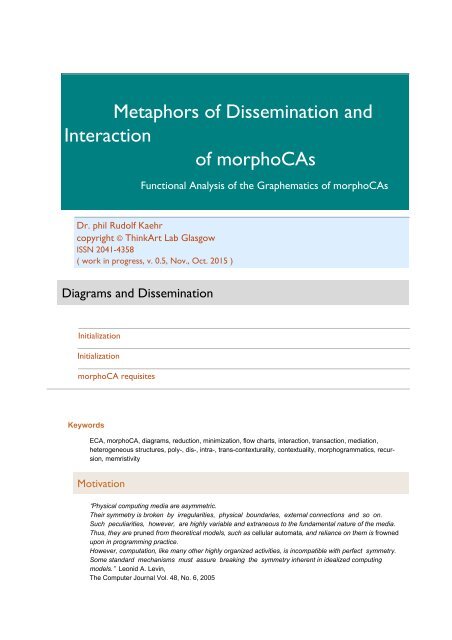
<strong>Metaphors</strong> <strong>of</strong> <strong>Dissemination</strong> <strong>and</strong><br />
<strong>Interaction</strong><br />
<strong>of</strong> <strong>morphoCAs</strong><br />
Functional Analysis <strong>of</strong> the Graphematics <strong>of</strong> <strong>morphoCAs</strong><br />
Dr. phil Rudolf Kaehr<br />
copyright © ThinkArt Lab Glasgow<br />
ISSN 2041-4358<br />
( work in progress, v. 0.5, Nov., Oct. 2015 )<br />
Diagrams <strong>and</strong> <strong>Dissemination</strong><br />
Initialization<br />
Initialization<br />
morphoCA requisites<br />
Keywords<br />
ECA, morphoCA, diagrams, reduction, minimization, flow charts, interaction, transaction, mediation,<br />
heterogeneous structures, poly-, dis-, intra-, trans-contexturality, contextuality, morphogrammatics, recursion,<br />
memristivity<br />
Motivation<br />
“Physical computing media are asymmetric.<br />
Their symmetry is broken by irregularities, physical boundaries, external connections <strong>and</strong> so on.<br />
Such peculiarities, however, are highly variable <strong>and</strong> extraneous to the fundamental nature <strong>of</strong> the media.<br />
Thus, they are pruned from theoretical models, such as cellular automata, <strong>and</strong> reliance on them is frowned<br />
upon in programming practice.<br />
However, computation, like many other highly organized activities, is incompatible with perfect symmetry.<br />
Some st<strong>and</strong>ard mechanisms must assure breaking the symmetry inherent in idealized computing<br />
models.” Leonid A. Levin,<br />
The Computer Journal Vol. 48, No. 6, 2005
2 Diagram.nb<br />
Minimization <strong>and</strong> flow charts<br />
It is not easy to explain how to underst<strong>and</strong> the results <strong>of</strong> <strong>morphoCAs</strong>. It seems that there is a strong conflict between<br />
the millions <strong>of</strong> visualizations, sonifications <strong>and</strong> structurations managed by the approach <strong>of</strong> claviatures <strong>and</strong> the<br />
paradigmatic statement developed in the paper "Asymmetric Palindromes" for <strong>morphoCAs</strong> that “What you see is not<br />
what it is”.<br />
Instead <strong>of</strong> studying the multitude <strong>of</strong> the products <strong>of</strong> <strong>morphoCAs</strong>, another approach that is more focused on the<br />
mechanism <strong>of</strong> the production process <strong>of</strong> <strong>morphoCAs</strong> might help to uncover the deep-structural significance <strong>of</strong><br />
morphogrammatic based cellular automata.<br />
This paper <strong>of</strong>fers some insights into the mechanism <strong>of</strong> production by the application <strong>of</strong> reductions (minimizations) <strong>of</strong><br />
the functional interpretations <strong>of</strong> the morphoCA rules <strong>and</strong> by designing the network <strong>of</strong> the actions <strong>of</strong> the morphic<br />
automata by some flow charts.<br />
There is not yet an algorthmic approach to reduce morphic CA functions accessible. But the distinction between<br />
reducible <strong>and</strong> non-reducible <strong>morphoCAs</strong> is well defined.<br />
Hence, instead <strong>of</strong> considering the multi-millions <strong>of</strong> morphoCA productions, some specific flow charts <strong>of</strong> the mechanism<br />
<strong>of</strong> production is presented to continue the studies <strong>of</strong> <strong>morphoCAs</strong>. With that a kind <strong>of</strong> reflection a kind <strong>of</strong> a metatheory<br />
<strong>of</strong> <strong>morphoCAs</strong> is introduced.<br />
From this meta-theoretial point <strong>of</strong> view, <strong>morphoCAs</strong> might be involved into an introspection between Kaluzhnine-<br />
Graph-Schemata <strong>of</strong> recursivity <strong>and</strong> poly-contextural memristivity.<br />
A further approach to study the deep-structure <strong>of</strong> the meaning <strong>of</strong> <strong>morphoCAs</strong> will be sketched in a further paper by<br />
an analysis <strong>of</strong> their underlying poly-contextural logics.<br />
Contexturality vs. contextuality<br />
The term “polycontexturality” occurs frequently in sociological studies. Often as a synonyme or replacement <strong>of</strong><br />
‘polycentricity’ <strong>and</strong> linguistically, modal-logically or semiotically identified with ‘contextuality’.<br />
Polycontexturality refers to a trans-classical paradigm <strong>of</strong> thinkind <strong>and</strong> writing that is not compatible with established<br />
concepts <strong>of</strong> science, while ‘polycentricity’ <strong>and</strong> ‘contextuality’ are parts <strong>of</strong> classical logic (say, modal logic), ontology<br />
<strong>and</strong> semiotics.<br />
“Polycentricity is similar to the concept <strong>of</strong> polycontexturality in logic. Polycontexturality represents a manysystem<br />
logic, in which the classical logic systems (called contextures) interplay with each other, resulting in<br />
a complexity that is structurally different from the sum <strong>of</strong> its components (Kaehr <strong>and</strong> Mahler 1996).”<br />
(Rajendra Singh, Towards Information Polycentricity Theory: Investigation <strong>of</strong> a Hospital Revenue Cycle,<br />
2011)<br />
A similar approach, chosen out <strong>of</strong> the ‘polycentricity or centextualist movement’, is proposed e.g. by Lars Qvortrup:<br />
“The implicit idea behind the first three theses is that we are on our way into a society, which is radically<br />
different from the so-called modern society. It has been described as “functionally differentiated” (Luhmann<br />
1997), as “polycontextural” (Günther 1979) or as “hypercomplex” (Qvortrup 1998), emphasising that it does<br />
not <strong>of</strong>fer one single point <strong>of</strong> observation, but a number <strong>of</strong> mutually competing observation points with each<br />
their own social context.”<br />
Lars Qvortrup, THE AESTHETICS OF INTERFERENCE: From anthropocentrism to polycentrism <strong>and</strong> the<br />
reflections <strong>of</strong> digital art<br />
http://www.hotelpr<strong>of</strong>orma.dk/Userfiles/File/artikler/lq.pdf<br />
It might provoke some progress if the distinctions proposed in this paper would be applied to systems theory <strong>of</strong> intra-,<br />
inter- <strong>and</strong> trans-contexturally mediated complex dis-contextural constellations <strong>and</strong> dynamics.<br />
http : // memristors.memristics.com Morphospheres Asymmetric %20 Palindromes.html<br />
http : // scholarworks.gsu.edu / cgi / viewcontent.cgi ? article = 1003 & context = ceprin_diss<br />
More entertainment with intra-, inter- <strong>and</strong> trans-disciplinarity <strong>of</strong> inter-, poly-, trans- <strong>and</strong> dis-contexturality at: “Modular<br />
Bolognese, Paradoxes <strong>of</strong> postmodern education” in: Short Studies 2008. Adventures in Diamond Strategies <strong>of</strong><br />
Change(s)<br />
http : // works.bepress.com / cgi / viewcontent.cgi ? article = 1007 & context = thinkartlab<br />
Three kinds <strong>of</strong> morphoCA diagrams
Diagram.nb 3<br />
Three kinds <strong>of</strong> morphoCA diagrams<br />
Three kinds <strong>of</strong> morphoCA diagrams have to be distinguished:<br />
1. Mono-contextural diagrams (intra)<br />
intra<br />
The first kind is covered by the classical diagrams. These diagrams hold for classical ECAs as much as for monocontextural<br />
<strong>morphoCAs</strong> <strong>of</strong> different topological complexity. Morphogrammatically, they are supported by the<br />
‘classical’ morphograms <strong>of</strong> complexity 2.<br />
2. Poly - contextural diagrams as interaction (inter, trans)<br />
The second kind is based on a distribution <strong>of</strong> the diagram <strong>of</strong> at least 3 loci. This distribution is basic for the interactions<br />
between otherwise autonomous automata. The internal structure <strong>of</strong> the memory/logic unit <strong>of</strong> the single<br />
automata is intrinsically changed toward a chiastic, i.e. memristive behavior <strong>of</strong> internal <strong>and</strong> external events.<br />
The interactional activity <strong>of</strong> the second kind <strong>of</strong> diagrams is supported by the morphograms <strong>of</strong> complexity 3.<br />
In this field <strong>of</strong> interactional activity <strong>of</strong> complexity 3, two different modi might be distinguished:<br />
• inter-actional with morphograms mg[5], mg[10] <strong>and</strong> mg[14], <strong>and</strong> head[{1,2,3}] -> i, i=1,2,3<br />
• trans-contextural mg[11], mg[12] <strong>and</strong> mg[13] with head [{1,2}] -> 3.<br />
3. Poly - contextural diagrams as mediation
4 Diagram.nb<br />
The third kind is based on the second kind but is involving the whole structural complexion <strong>of</strong> the distributed morpho-<br />
CAs. Only with this configuration the full graphematic character <strong>of</strong> <strong>morphoCAs</strong> enters the trans-classic game <strong>of</strong><br />
computation, interaction, reflection <strong>and</strong> mediation.<br />
Mediative actions are supported by morphograms <strong>of</strong> the minimal complexity 4, represented by the morphogram<br />
mg[15] with head[{1,2,3}]->4.<br />
Poly - contextural basic component<br />
inter<br />
intra<br />
trans<br />
intra<br />
Exam ples<br />
Functions<br />
intra : 0, 0, 0 → 0 : sys1, 1, 1 → sys1, 1, 1<br />
trans : 0, 0, 1 → 2 : sys1, 1, 1 → sys3 || sys1 || sys3<br />
inter : 1, 2, 1 → 0 : sys2, 1, 2 → sys1 || sys3 || sys1<br />
med : 1, 0, 2 → 3 : sys1, 2, 3 → sys5 || sys4 || sys6<br />
Action schemes<br />
intra iteration scheme<br />
t<br />
C k-1 , C t t<br />
k , C k+1<br />
C k t+1 ≡ C k<br />
t<br />
inter / trans - action scheme<br />
t<br />
C i,k-1<br />
t<br />
, C i,k , C i,k+1<br />
t<br />
t<br />
|| C j,k-1<br />
t<br />
, C j,k , C j,k+1 <br />
t+1<br />
C i,k ⟶ C t+1 t+1<br />
i,k ≡ C j,k<br />
t<br />
t<br />
C k-1 , C t t<br />
k , C k+1<br />
t<br />
C j,k-1<br />
t<br />
, C j,k , C j,k+1 <br />
t<br />
C k t+1 ≡ C k<br />
t<br />
Morphograms
Diagram.nb 5<br />
intra<br />
R1 R2 R3 R4<br />
■ ■ ■<br />
- ■ -<br />
■ ■ □<br />
- ■ -<br />
■ □ ■<br />
- ■ -<br />
■ □ □<br />
- ■ -<br />
R6 R7 R8 R9<br />
■ ■ ■<br />
- □ -<br />
■ ■ □<br />
- □ -<br />
■ □ ■<br />
- □ -<br />
■ □ □<br />
- □ -<br />
trans<br />
R11 R12 R13<br />
■ ■ □<br />
- ■ -<br />
■ □ ■<br />
- ■ -<br />
■ □ □<br />
- ■ -<br />
inter<br />
R5 R10 R14<br />
■ □ ■<br />
- ■ -<br />
■ □ ■<br />
- □ -<br />
■ □ ■<br />
- ■ -<br />
mediation<br />
R15<br />
■ □ ■<br />
- ■ -<br />
The compound morphogram ruleDM[{1, 3, 4, 11, 15}] inscribes the deep-structure <strong>of</strong> the mediation <strong>of</strong> intra- <strong>and</strong> intercontextural<br />
actions.<br />
■ ■ ■<br />
- ■ -<br />
■ □ ■<br />
- ■ -<br />
■ □ □<br />
- ■ -<br />
■ ■ □<br />
- ■ -<br />
■ □ ■<br />
- ■ -<br />
Poly-contextural logic<br />
Quite obviously, intra-contextural morphograms are representing the deep-structure <strong>of</strong> junctional mono- <strong>and</strong> polycontextural<br />
operators.<br />
As a first remark, inter- <strong>and</strong> trans-contextural morphograms are representing the deep-structures <strong>of</strong> transjunctional<br />
poly-contextural operators.<br />
Morphogram mg[15] represents the full differentiations <strong>of</strong> the interplay <strong>of</strong> inter- <strong>and</strong> trans-contextural poly-contextural<br />
operators.<br />
The pro<strong>of</strong>-theoretical metaphor <strong>of</strong> polycontextural interplays is not anymore just a ‘tree’ but a ‘forrest <strong>of</strong> colored trees’.<br />
Example: ternary 3-contextural transjunctions <strong>of</strong> ruleDCM[{1, 2, 12, 13, 5}]<br />
{0, 0, 0} → 0, {0, 0, 1} → 0 : dis - junctions in syst1,<br />
{0, 0, 2} → 0 : junction in syst3, "0⋀(0⋁2)≡ 0",<br />
{2, 2, 0} → 2 : junction in syst3, "2⋀(2⋁0)≡ 2",<br />
{0, 1, 0} → 2, {1, 0, 0} → 2 : trans - junctions from syst1 to sys2 || sys3,<br />
{1, 2, 1} → 0 : trans - junctions from syst2 to sys1 || sys3<br />
{0, 2, 2} → 1, {2, 0, 0} → 1 : trans - junctions from syst3 to sys1 || sys2,<br />
{0, 1, 2} → 0, {2, 1, 0} → 2 : trans - junctions from syst1, 3, 2 to sys1 || sys3<br />
1. Mono-contextural diagrams: ECA <strong>and</strong> morphoCA (m,2,n)
6 Diagram.nb<br />
1. Mono-contextural diagrams: ECA <strong>and</strong> morphoCA (m,2,n)<br />
Diagram <strong>of</strong> the ECA scheme<br />
K. Salman’s paper “Elementary Cellular Automata (ECA) Research platform” gives an elaborated definition <strong>and</strong><br />
explanation <strong>of</strong> the concept <strong>of</strong> ECAs.<br />
For the purpose <strong>of</strong> an introduction <strong>of</strong> <strong>morphoCAs</strong> it suffice to connect to some <strong>of</strong> its terms <strong>and</strong> constructions.<br />
“For ease <strong>of</strong> illustration we let the CA evolve according to one uniform neighborhood transition function <strong>and</strong><br />
fixed radius which is a local function (rule) 3 0 : 4 2 r+1 ⟶ 4 where the CA evolves after a certain number <strong>of</strong><br />
time steps T.<br />
In this case we have a total <strong>of</strong> 5 2 r+1 distinct rules. It follows that a 1 - D CA is a linear lattice or register <strong>of</strong> 6∈<br />
N memory cells. Each cell is represented by C k<br />
t , where 9 = [1: 6], 6∈ N <strong>and</strong> : = [1: ;], ;∈ Z that<br />
describes the content <strong>of</strong> memory location at evolution time step t..” (K. Salman)<br />
Figure 5, Detailed Structure <strong>of</strong> a typical Cellular Automaton Cell for rule 30.<br />
http : // www.cyberjournals.com/Papers/Jun2013/02. pdf<br />
Diagram <strong>of</strong> the CA rule in respect <strong>of</strong> input <strong>and</strong> output cells in time t to t+1<br />
move right<br />
http : // www.slideshare.net / ijcsit / 5413 ijcsit03<br />
Description <strong>of</strong> the mechanism <strong>of</strong> the CA calculation<br />
The object D k <strong>of</strong> C k<br />
t+1<br />
<strong>of</strong> Fig. 5 is a result <strong>of</strong> the calculation <strong>of</strong> the logical unit U, i.e. Transition Rule Logic, in relation<br />
t t<br />
to its inputs C k+1 <strong>and</strong> C k-1 , but it is also at the same time the initial value, Q k , in the Memory Cell, <strong>of</strong> a new calculation<br />
<strong>of</strong> a next step <strong>of</strong> the CA.<br />
This new calculation might happen intra-contexturally as a mapping from Q k as Q i to the logic unit U i or transcontexturally<br />
as a mapping from Q k as Q i to the new object D k <strong>of</strong> D k<br />
i+1<br />
in CA 2.1 where it becomes the new value <strong>of</strong><br />
Q k i+1 for a calculation in CA 2.2 .<br />
The presumption <strong>of</strong> the classical model <strong>of</strong> ECAs is certainly that all components are from the same contexture, <strong>and</strong><br />
having the same clock.<br />
Mono-contextural CAs are homogeneous structures.
Diagram.nb 7<br />
Classical Cellular Automata. Homogeneous Structures<br />
By V. Z. Aladjev<br />
intra iteration scheme<br />
[Ct k-1 , C t k , Ct<br />
k+1<br />
C k t+1 ≡ C k<br />
t<br />
Ct k-1 , C t k , Ct<br />
k+1<br />
C k t+1<br />
≡ C k<br />
t<br />
inter / trans interaction scheme<br />
Ct<br />
i,k-1<br />
, Ct<br />
i,k , Ct<br />
i,k+1<br />
] || Ct<br />
j,k-1<br />
, Ct<br />
j,k , Ct<br />
j,k+1 <br />
Ct+1 i,k ⟺ intertrans<br />
C t+1 j,k ≡ Ct<br />
j,k<br />
intra<br />
Ct<br />
j,k-1<br />
, Ct<br />
j,k , Ct<br />
j,k+1<br />
<br />
inter / trans interaction network scheme<br />
Ct<br />
i,k-1<br />
, Ct<br />
i,k , Ct<br />
i,k+1<br />
] || Ct<br />
j,k-1<br />
, Ct<br />
j,k , Ct<br />
j,k+1 || [Ct<br />
h,k-1 , Ct<br />
h,k , C h,k+1<br />
t<br />
]<br />
⟺<br />
C t+1 i,k ≡ Ct<br />
i,k<br />
⟺ intertrans<br />
C t+1 j,k ≡ Ct j,k ⟺ intertrans<br />
C t+1 h,k ≡ Ct<br />
h,k<br />
⟺<br />
intra<br />
Ct<br />
i,k-1 , Ct i,k ,<br />
Ct<br />
i,k+1<br />
|| Ct<br />
j,k-1<br />
, Ct<br />
j,k , Ct<br />
j,k+1<br />
|| Ct<br />
h,k-1<br />
, Ct<br />
h,k , Ct<br />
h,k+1<br />
<br />
Diagram <strong>of</strong> the sub-rule definition <strong>of</strong> ECAs<br />
A sub-rule implementation <strong>of</strong> the ECA rules might augment its computational efficiency <strong>and</strong> reduce numeric complexity<br />
for programmable hybrid ECA compositions.<br />
As it is well known, CAs are understood as parallel computing concepts <strong>and</strong> devices.<br />
There is no doubt that the sketched sub-rule appoach can be concretized <strong>and</strong> implemented as a ‘hybrid’ ECA on a<br />
hardware board like Spartan-6 FPGA Connectivity Kit or similar.<br />
(http://www.xilinx.com/products/boards-<strong>and</strong>-kits.html)<br />
A further step in augmenting the granularity <strong>of</strong> CAs might be achieved with the sub-rule approach for ECA rules.<br />
Each ECA rule is defined in a sub-rule oriented approach as a composition <strong>of</strong> sub-rules. Thus all compatible subrules<br />
can be applied in parallel to realize a single ECA rule.<br />
Also the sub-rule approach is defining the ECA rules is not yet showing the flow chart <strong>of</strong> the interactions <strong>of</strong> the subrules<br />
to build the ECA rule.<br />
ECA-rule = [eca1, eca2, ..., eca8]<br />
Example: ECA rule 210
8 Diagram.nb<br />
t<br />
C k-1 , C t k ,<br />
t<br />
C k+1<br />
t+1<br />
C k<br />
: intra<br />
ruleECA[{6, 7, 3, 9, 10, 12, 13, 15}]<br />
{{0, 0, 0} → 1,<br />
{0, 0, 1} → 1,<br />
{0, 1, 0} → 0,<br />
{0, 1, 1} → 1,<br />
{1, 0, 0} → 0,<br />
{1, 0, 1} → 0,<br />
{1, 1, 0} → 1,<br />
{1, 1, 1} → 0}<br />
210<br />
FromDigits[{1, 1, 0, 1, 0, 0, 1, 0}, 2]<br />
Hence the ECA rule 210 is represented by the tuple (6,7,3,9,10,12,13,15) <strong>of</strong> ECA sub-rules.<br />
Flow chart <strong>of</strong> the parallel realization <strong>of</strong> the 8 sub - rules <strong>of</strong> an ECA.<br />
“If in a CA the same rule applies to all cells, then the CA is called a uniform CA; otherwise the CA is called a hybrid<br />
CA (Fig. 1).”<br />
Theory <strong>and</strong> Applications <strong>of</strong> Cellular Automata in Cryptography<br />
S.N<strong>and</strong>i, B.K.Kar <strong>and</strong> P.Pal Chaudhuri<br />
ECA sub-rule manipulators<br />
The method <strong>of</strong> sub-rules for ECAs is an abstraction <strong>and</strong> parametrization <strong>of</strong> the components <strong>of</strong> the rule schemes that<br />
allows a micro-anlysis <strong>of</strong> the ECAs. The ECA sub-rule manipulator manages all ECA rules <strong>of</strong> a 1D ECA. The subrule<br />
manipulators enables a micro-analysis <strong>of</strong> the behavior <strong>of</strong> all 2 8 ECA rules.<br />
Each 1-D ECA rule number has a sub-rule number representation. There are just 8 disjunct pairs <strong>of</strong> sub-rules to<br />
define a 1D ECA rule.<br />
The results are visualized below. The combination <strong>of</strong> the 8 sub-rules covers all the 256 well known ECA rules.
Diagram.nb 9<br />
k 1 6<br />
l 2 7<br />
m 3 8<br />
n 4 9<br />
o 5 10<br />
p 11 12<br />
q 13 14<br />
r 15 16<br />
steps 44<br />
Mono-contextural ruleDCKF (5,2,3)<br />
a 1111 1112<br />
b 1121 1122<br />
c 1211 1212<br />
d 2111 2112<br />
e 1221 1222<br />
f 2121 2122<br />
g 2212 2211<br />
h 2221 2222<br />
steps 22<br />
mesh<br />
Reduction (trivial)<br />
ruleDCKF[{1111, 1122, 1211, 2112, 1221, 2121, 2211, 2222}]
10 Diagram.nb<br />
intra<br />
{1, 1, 1, 1} → 1, {0, 0, 0, 0} → 0, : Sys1<br />
{1, 1, 1, 0} → 0, {0, 0, 0, 1} → 1,<br />
{1, 1, 0, 1} → 1, {0, 0, 1, 0} → 0,<br />
{1, 0, 1, 1} → 0, {0, 1, 0, 0} → 1,<br />
{1, 1, 0, 0} → 1, {0, 0, 1, 1} → 0,<br />
{1, 0, 1, 0} → 1, {0, 1, 0, 1} → 0,<br />
{1, 0, 0, 1} → 1, {0, 1, 1, 0} → 0,<br />
{1, 0, 0, 0} → 0, {0, 1, 1, 1} → 1<br />
R<strong>and</strong>om<br />
Scheme: (r1, r2, r3, r4) ⟹ r5, r i = {0, 1}<br />
r3<br />
r5<br />
r1r2<br />
ruleDCKF<br />
r4<br />
2. Poly-contextural diagrams with interactions<br />
General approach<br />
Internal structure <strong>of</strong> the memory unit <strong>of</strong> the second kind<br />
Following for example K. Salman’s classical modelling approach in “Elementary Cellular Automata (ECA) Research<br />
platform“ a more explicit modelling <strong>of</strong> the mechanism <strong>of</strong> <strong>morphoCAs</strong> might be achieved.<br />
A first crucial difference to the classical concept is the fact that the memory unit is not just passively receiving (D) <strong>and</strong><br />
sending data (Q) but is also actively deciding to which system <strong>of</strong> its computational environment they belong <strong>and</strong> if the<br />
data remain in its domain or not. If not, the activity <strong>of</strong> the memory unit is deciding where that data belong <strong>and</strong> sends it<br />
to the evoked computational unit <strong>of</strong> the complexion.<br />
In terms <strong>of</strong> actors, the memory unit is receiving, sending <strong>and</strong> deciding about the contextures <strong>of</strong> data. Classical<br />
memory actions are strictly intra-contextural. This holds in the same sense for multi-processor systems too. They are<br />
acting strictly intra-contexturally, keeping their distributed data together.<br />
Hence, the logic devices in the modified diagram, Fig. 5b, have two function towards its memory units:<br />
1. a decision operation over the logical operations, i.e. to decide if an operation stays inside the contexture or if it<br />
leaves trans-contexturally the contexture for another contexture on another layer <strong>of</strong> the complex poly-layered<br />
morphoCA system.<br />
2. the intra-contextural function <strong>of</strong> producing the junctional values for the corresponding intra-contextural memory in<br />
the sense <strong>of</strong> ordinary logical functions, like NAND or NOR.
Diagram.nb 11<br />
Hence, the logic devices in the modified diagram, Fig. 5b, have two function towards its memory units:<br />
1. a decision operation over the logical operations, i.e. to decide if an operation stays inside the contexture or if it<br />
leaves trans-contexturally the contexture for another contexture on another layer <strong>of</strong> the complex poly-layered<br />
morphoCA system.<br />
2. the intra-contextural function <strong>of</strong> producing the junctional values for the corresponding intra-contextural memory in<br />
the sense <strong>of</strong> ordinary logical functions, like NAND or NOR.<br />
The object D k <strong>of</strong> the CA diagram receives a value from the logic unit <strong>and</strong> it delivers it to Q as Q k for the new calculation<br />
with c k <strong>of</strong> the logical unit in time t + 1.<br />
Secondly, Q receives the value from D as a value, not for Q 1.1 in CA 1 but for Q 2.1 <strong>of</strong> the neighbor layer CA 2 . This new<br />
value is memorized in the neighbor CA 2 as the new positive value for calculation in CA 2 , hence it is placed in<br />
CA 2.1 <strong>and</strong> not as a genuine value <strong>of</strong> CA 2 as CA 2.2 .<br />
The result <strong>of</strong> the application <strong>of</strong> the rule in all 3 sub-systems is delivered with the multi-layered system as a whole, i.e.<br />
with morphoCA (3,3) <strong>and</strong> its rules R (3,3) .<br />
Obviously, the whole automaton with its different layers has to be designed in the epistemological mode <strong>of</strong> the ‘asabstraction’,<br />
i.e. as “A as B is C” <strong>and</strong> not in the mode <strong>of</strong> identity with “A is A”.<br />
The modified diagram is introducing an environment to the original mono-contextural CA diagram that implies<br />
the possibility <strong>of</strong> interactions. The environment <strong>of</strong> a CA system is the primary condition for a possible selfreflection<br />
<strong>of</strong> the complex system <strong>of</strong> different <strong>and</strong> interacting CAs.<br />
The logic behind this construction was first introduced by Gotthard Gunther’s “Cognition <strong>and</strong> Volition” (1970)<br />
which gives a pr<strong>of</strong>ound explanation <strong>of</strong> the new concept <strong>of</strong> the ‘proemial relation’.<br />
Modified diagram Fig. 5b<br />
Memristive properties <strong>of</strong> the memory/logic unit<br />
Why <strong>and</strong> how is the behavior <strong>of</strong> the memory units <strong>of</strong> <strong>morphoCAs</strong> <strong>of</strong> second-order <strong>and</strong> memristive <strong>and</strong> not just<br />
defined as first-order actions <strong>of</strong> storage <strong>and</strong> transformations? The main strategy <strong>of</strong> the whole maneuver is to avoid<br />
‘information processing’. <strong>Interaction</strong> is prior to information exchange.<br />
It could be said: <strong>morphoCAs</strong> without memristivity are reducible without loss to classical CAs.<br />
internal :<br />
external :<br />
D k 1.1 ⟹<br />
1.1 2.2<br />
Q k > k<br />
⇵ ⇵<br />
U 1.1 → D k 1.1 ⟹<br />
1.1<br />
Q k > 2.2 k ⟶ 4 2.2 k : C 2.1 k → U 2.2<br />
⇕ ⇵<br />
Q k 1.2 ⟹ Q k<br />
2.1<br />
Q k 1.2 ⟹ Q k<br />
2.1<br />
The diagram below, Fig. 1, shows again the chiastic interaction between operators (M) <strong>and</strong> oper<strong>and</strong>s ‘σ’ distributed<br />
over different loci <strong>of</strong> the kenomic matrix.<br />
“M as σ” is obviously not the so called self-reference <strong>of</strong> “M is σ”.<br />
Χ (M, σ) =<br />
M 1.1 ⟹σ 2.1 M 2.2 ⟹σ 1.2<br />
x<br />
σ 2.2 ⟹M 1.2 σ 1.1 ⟹M 2.1<br />
http : //<br />
memristors.memristics.com / semi - Thue / Notes %20 on %20 semi - Thue %20 systems.html<br />
Fig . 1 Chiasm (M, σ)
12 Diagram.nb<br />
Explanation <strong>of</strong> Fig. 1<br />
"The wording here is not only<br />
" types becomes terms <strong>and</strong> terms becomes types " but<br />
“ a type as a term becomes a term " <strong>and</strong>, at the same time,<br />
"a type as type remains a type".<br />
Thus, "a type as a term becomes a term <strong>and</strong> as a type it remains a type".<br />
And the same round for terms.<br />
Full wording for a chiasm between terms <strong>and</strong> types over two loci<br />
Explicitly, first the green round,<br />
"A type σ 1.1 as a term M 2.1 becomes a term M 2.1<br />
<strong>and</strong> as a type σ 1.1 it remains a type σ 1.1 for a term M 1.1 ".<br />
And,<br />
"A type σ 2.2 as a term M 1.2 becomes a term M 1.2<br />
<strong>and</strong> as a type σ 2.2 it remains a type σ 2.2 for a term M 2.2 ".<br />
And simultaneously, mediated,<br />
the second round in red, the same for terms:<br />
"A term M 1.1 as a type σ 2.1 becomes a type σ 2.1<br />
<strong>and</strong> as a term M 1.1 it remains a term M 1.1 for a type σ 1.1 ".<br />
And,<br />
"A term M 2.2 as a type σ 1.2 becomes a type σ 1.2<br />
<strong>and</strong> as a term M 2.2 it remains a term M 2.2 for a type σ 2.2 ".<br />
And finally, between terms M 1.1 <strong>and</strong> M 2.2 <strong>and</strong> types σ 1.1 <strong>and</strong> σ 2.2 ,<br />
a categorial coincidence is realized.<br />
While between terms <strong>and</strong> types a morphism (order relation) exists.<br />
Fig . 2 Complete interactional scheme
Diagram.nb 13<br />
interaction scheme<br />
t<br />
C i,k-1<br />
t<br />
, C i,k , C i,k+1<br />
t<br />
t<br />
|| C j,k-1<br />
t<br />
, C j,k , C j,k+1 <br />
t<br />
t+1<br />
C i,k<br />
⟶<br />
C t+1 t<br />
j,k ≡ C j,k<br />
t<br />
C j,k-1<br />
t<br />
, C j,k , C j,k+1<br />
<br />
t<br />
Hence, this kind <strong>of</strong> memory is a complexion <strong>of</strong> ‘memory’ <strong>and</strong> ‘logic’ as it is supposed for memristive behavior.<br />
There are four basic components plus the clock in the interaction paradigm <strong>of</strong> <strong>morphoCAs</strong>.<br />
Calculation :<br />
sendreceive,<br />
acceptreject<br />
in generalized time<br />
In contrast to the classical CA with its send/receive properties, there are four basic components plus the clock in the<br />
paradigm <strong>of</strong> <strong>morphoCAs</strong>. The sens/receive or read/write mechanism is augmented in <strong>morphoCAs</strong> by a decisionmaking<br />
(trans-logical) component <strong>of</strong> accept/reject in regard <strong>of</strong> the sub-system property.<br />
The contrast to Konrad Zuse's conception <strong>of</strong> calculation is obvious :<br />
“Rechnen heisst : Aus gegebenen Angaben nach einer Vorschrift neue Angaben bilden.” (Konrad Zuse)<br />
The discontexturaliy <strong>of</strong> <strong>morphoCAs</strong> is certainly also not in hamony with Karl Hewitt’s monolithic actor approach to<br />
computation.<br />
A systematic deconstruction has obviously to deconstruct all 4+1 components <strong>of</strong> the diagram.<br />
The very first deconstruction happens by parametrizing the inputs. Each input/output, i.e. send/receive action might<br />
belong to a different contexture. Hence, the very first task <strong>of</strong> the automaton is to h<strong>and</strong>le such pr<strong>of</strong>ound diversity. This<br />
job is obsolete for classical CAs because all data are from/in the same contexture.<br />
This contextural embodiment <strong>of</strong> the fourth term, C k<br />
t+1 , explains why the term is not just an extensional result <strong>of</strong> a<br />
mapping but is structurally depending on the conceptual ‘history’ <strong>of</strong> the 3 previous actions.<br />
This underst<strong>and</strong>ing <strong>of</strong> the morphoCA rules relates back to the concept <strong>of</strong> the ϵ/ν-structure <strong>of</strong> morphic objects <strong>and</strong><br />
actions within the concept <strong>of</strong> the proposed memristive automata.<br />
http : // www.thinkartlab.com / pkl / media / SKIZZE - 0.9<br />
http : // works.bepress.com / thinkartlab / 20 /<br />
http : // transhumanism.memristics.com / Diagrammatik.ppt.htm<br />
.5 - medium.pdf<br />
From memristive flip-flop to memristive interactions<br />
Finite state machines <strong>and</strong> <strong>morphoCAs</strong><br />
“A Cellular Automaton (CA) is an infinite, regular lattice <strong>of</strong> simple finite state machines that change their states<br />
synchronously, according to a local update rule that specifies the new state <strong>of</strong> each cell based on the old states<br />
<strong>of</strong> its neighbors.” (Kari)<br />
http://users.utu.fi/jkari/ca/CAintro.pdf<br />
“Furthermore, since the ECA is actually a finite state machine then the present state <strong>of</strong> the neighborhood<br />
C k-1 , C t t t t+1<br />
t<br />
k , C k+1 <strong>of</strong> cell C k at time step t <strong>and</strong> the next state C k at time step t + 1, can be analyzed<br />
by the state transition table <strong>and</strong> the state diagram depicted in figure 4.” (K. Salman)
14 Diagram.nb<br />
“Furthermore, since the ECA is actually a finite state machine then the present state <strong>of</strong> the neighborhood<br />
C k-1 , C t t t t+1<br />
t<br />
k , C k+1 <strong>of</strong> cell C k at time step t <strong>and</strong> the next state C k at time step t + 1, can be analyzed<br />
by the state transition table <strong>and</strong> the state diagram depicted in figure 4.” (K. Salman)<br />
Figure 4, state machine analysis <strong>of</strong> Rule 30<br />
http : // www.slideshare.net / ijcsit / 5413 ijcsit03<br />
ECA Rule 30<br />
FromDigits[{0, 0, 0, 1, 1, 1, 1, 0}, 2]<br />
30<br />
FromDigits[kAryFromRuleTable[<br />
ruleECA[{1, 2, 3, 9, 5, 11, 13, 15}]], 2]<br />
30<br />
ruleECA[{1, 2, 3, 9, 5, 11, 13, 15}] = rule30<br />
rule30 111 110 101 100 011 010 001 000<br />
1 - - - (5) : 1 (9) : 1 (3) : 1 (2) : 1 -<br />
0 (15) : 0 (13) : 0 (11) : 0 - - - - (1) : 0<br />
http : // memristors.memristics.com / MorphoFSM / Finite<br />
%20 State %20 Machines %20 <strong>and</strong> %20 Morphogrammatics.html<br />
System <strong>of</strong> elementary kenomic cellular automata rules in trito-difference form<br />
R1 R2 R3 R4<br />
R5<br />
■ ■ ■<br />
- ■ -<br />
■ ■ □<br />
- ■ -<br />
■ □ ■<br />
- ■ -<br />
■ □ □<br />
- ■ -<br />
■ □ ■<br />
- ■ -<br />
R6 R7 R8 R9<br />
R10<br />
■ ■ ■<br />
- □ -<br />
■ ■ □<br />
- □ -<br />
■ □ ■<br />
- □ -<br />
■ □ □<br />
- □ -<br />
■ □ ■<br />
- □ -<br />
R11 R12 R13 R14 R15<br />
■ ■ □<br />
- ■ -<br />
■ □ ■<br />
- ■ -<br />
■ □ □<br />
- ■ -<br />
■ □ ■<br />
- ■ -<br />
■ □ ■<br />
- ■ -
Diagram.nb 15<br />
e1 e2 e4<br />
- e3 e5<br />
R1 - e6<br />
e1 e2 v4<br />
- e3 v5<br />
R6 - v6<br />
e1 v2 v4<br />
- v3 v5<br />
R11 - v6<br />
e1 v2 e4<br />
- v3 e5<br />
R2 - v6<br />
e1 v2 v4<br />
- v3 v5<br />
R7 - e6<br />
v1 e2 v4<br />
- v3 v5<br />
R12 - v6<br />
v1 e2 e4<br />
- v3 v5<br />
R3 - e6<br />
v1 v2 v4<br />
- e3 e5<br />
R8 - v6<br />
v1 v2 e4<br />
- v3 v5<br />
R13 - v6<br />
v1 v2 e4<br />
- e3 v5<br />
R4 - v6<br />
v1 v2 v4<br />
- e3 e5<br />
R9 - e6<br />
v1 v2 v4<br />
- v3 e5<br />
R14 - v6<br />
v1 v2 v4<br />
- e3 v5<br />
R5 - v6<br />
v1 v2 v4<br />
- v3 v5<br />
R10 - e6<br />
v1 v2 v4<br />
- v3 v5<br />
R15 - v6<br />
Interpretation<br />
Difference scheme<br />
The difference scheme is a scheme <strong>of</strong> differences, <strong>and</strong> not just a relational mapping from C 3 to C.<br />
Also an evolution from [Ct k-1 , C kt , Ct<br />
k+1 ] to Ct+1 k is defined by all previous elements <strong>of</strong> time t <strong>of</strong> the specified<br />
CA rule there is no concrete differentiation between the new state <strong>of</strong> Ct+1 k <strong>and</strong> the previous states defined.<br />
Hence, the new state C k<br />
t+1 <strong>of</strong> a classical CA might incorporate any arbitrary value from a pre-given set <strong>of</strong> values<br />
<strong>and</strong> is not retro-recursive characterized by the differences <strong>of</strong> the previous constellation it depends.<br />
C k-1 , C t k ,<br />
t<br />
C k+1<br />
t+1<br />
C k<br />
⟹<br />
t<br />
C k-1 , C t t<br />
k , C k+1<br />
t+1<br />
C k<br />
⟹<br />
d1 d2 d4<br />
- d3 d5<br />
- - d6<br />
, with d = {ϵ, ν}, ϵ = equal, ν = non-equal<br />
FSA Example<br />
t<br />
d1 = diff ( C k-1 , C t k ),<br />
t t<br />
d2 = diff ( C k-1 , C k+1 ),<br />
d3 = diff ( C t t<br />
k , C k+1 ),<br />
t<br />
d4 = diff ( C k-1 , C t+1 k ),<br />
t<br />
d5 = diff ( C k+1 , C t+1 k ),<br />
d6 = diff ( C t k , C t+1 k ).<br />
FSA(aabc)<br />
MorphoFSA[aabc]
16 Diagram.nb<br />
http : // memristors.memristics.com / CA -<br />
Overview / Short - %20 Overview %20 <strong>of</strong> %20 Cellular %20 Automata.pdf<br />
Monomorphic prolongation<br />
First aspect: iteration<br />
Given a morphogram MG, which is always a localized pattern in a kenomic matrix, a prolongation (successor,<br />
evolution) <strong>of</strong> the morphogram is achieved with the successor operator s i . To each prolongation a further prolongation<br />
is defined by the iterated application <strong>of</strong> the operator s i .<br />
The morphogrammatic succession MG ⟶ s i<br />
MG is founded by its model gm ⟶ h j<br />
gm <strong>and</strong> the morphism f, guaranteeing<br />
the commutativity <strong>of</strong> the construction.<br />
As a third rule, the iterability <strong>of</strong> the successor operation is arbitrary, which is characterised by the commutativity <strong>of</strong><br />
the diagram. Hence, the conditions for a (retrograde) recursive formalisation are given.<br />
Second aspect: anti-dromicity<br />
Each prolongation is realized simultaneously by an iterative progression <strong>and</strong> an antidromic retro-gression. That is,<br />
the operation <strong>of</strong> prolongation <strong>of</strong> a morphogram is defined retro-grade by the possibilities given by the encountered<br />
morphogram. A concrete prolongation is selecting out <strong>of</strong> those possibilities its specific successions. All successions<br />
are to be considered as being realized at once.<br />
Third aspect: simultaneity <strong>and</strong> interchangeability<br />
This simultaneity <strong>of</strong> different successions defines the range <strong>of</strong> the prolongation. This definition <strong>of</strong> morphogrammatic<br />
prolongation is not requiring an alphabet <strong>and</strong> a selection <strong>of</strong> a sign out <strong>of</strong> the alphabet. Hence, the concept <strong>of</strong> morphogrammatic<br />
prolongation is defined by the two aspects <strong>of</strong> iteration <strong>and</strong> antidromic retro-gradeness <strong>of</strong> the successor<br />
operation. The simultaneity <strong>of</strong> the prolongations is modeled by the interchangeability <strong>of</strong> its actions.<br />
Fourth aspect: diamond characterization <strong>of</strong> antidromicity<br />
Both aspects together, repeatability <strong>and</strong> antidromicity with its simultaneous <strong>and</strong> interchangeable realizations, are<br />
covered by the diamond-theoretic concept <strong>of</strong> combination <strong>of</strong> operations <strong>and</strong> morphisms, i.e. composition <strong>and</strong><br />
saltisition, between morphogramatic prolongations.<br />
The philosophical status <strong>of</strong> <strong>morphoCAs</strong> has yet to be determined.“What’s after digitalism?” might give a hint.<br />
https : // www.academia.edu / 1 873 531 / Digital_Philosophy._Formal<br />
_Ontology _<strong>and</strong> _Knowledge _Representation _in _Cellular _Automata<br />
Internal structure <strong>of</strong> the morphogrammatic transition rule<br />
Recall definitions: classical transition rule<br />
"Rigid computations have another node parameter: location or cell. Combined with time, it designates the<br />
event uniquely. Locations have structure or proximity edges between them. They (or their short chains)<br />
indicate all neighbors <strong>of</strong> a node to which pointers may be directed.<br />
“CA are a parallel rigid model. Its sequential restriction is the Turing Machine (TM). The configuration <strong>of</strong> CA<br />
is a (possibly multi-dimensional) grid with a fixed (independent <strong>of</strong> the grid size) number <strong>of</strong> states to label<br />
the events. The states include, among other values, pointers to the grid neighbors. At each step <strong>of</strong> the<br />
computation, the state <strong>of</strong> each cell can change as prescribed by a transition function <strong>of</strong> the previous states<br />
<strong>of</strong> the cell <strong>and</strong> its pointed-to neighbors. The initial state <strong>of</strong> the cells is the input for the CA. All subsequent<br />
states are determined by the transition function (also called program)." Leonid A. Levin. Fundamentals <strong>of</strong><br />
Computing.
“CA are a parallel rigid model. Its sequential restriction is the Turing Machine (TM). The configuration <strong>of</strong> CA<br />
is a (possibly multi-dimensional) grid with a fixed (independent <strong>of</strong> the grid size) number <strong>of</strong> states to label<br />
the events. The states include, among other values, pointers to the grid neighbors. At each step <strong>of</strong> the<br />
Diagram.nb 17<br />
computation, the state <strong>of</strong> each cell can change as prescribed by a transition function <strong>of</strong> the previous states<br />
<strong>of</strong> the cell <strong>and</strong> its pointed-to neighbors. The initial state <strong>of</strong> the cells is the input for the CA. All subsequent<br />
states are determined by the transition function (also called program)." Leonid A. Levin. Fundamentals <strong>of</strong><br />
Computing.<br />
http://www.cs.bu.edu/fac/lnd/toc/z/z.html<br />
Morphogrammatic transition rule<br />
http : // memristors.memristics.com / Memristive %20<br />
Cellular %20 Automata / Memristive %20 Cellular %20 Automata.html<br />
General scheme<br />
rule set, start string<br />
string pos = (Nr., l)<br />
ReLabel<br />
ReLabel (string)<br />
↙ ↘ NextGen<br />
NextGen (ReLabel (string))<br />
↘ ↓ ↙ ∈ rule - set?<br />
〈yes; no〉<br />
apply rule<br />
result<br />
Example<br />
rule set = {1, 7, 8, 4}, start string<br />
[bcb] : string at pos (Nr., l)<br />
ReLabel<br />
[aba]<br />
↙ ↘ NextGen<br />
[abaa][abab][abac]<br />
↘ ↓ ↙ [abaa] ∈ rule - set?<br />
〈yes; no〉<br />
apply : [abaa] rule7<br />
result = [a]<br />
NextGen is in this morphoCA context a retrograde recursive action <strong>and</strong> not to be confued by a classical recursion.<br />
What makes the difference?<br />
1. retro - grade recursivity<br />
2. irreducible heterogeneity<br />
3. interactivity <strong>and</strong> reflectionality<br />
Morphogrammatic example<br />
evol i (MG) :<br />
∀ i ∈ (mg (MG)), 1 ≤ i ≤ mg (MG) + 1<br />
second<br />
selection<br />
retrogression<br />
first<br />
choice<br />
([mg 1 ... mg i ... mg n ] ⟶ [mg 1 ... mg i .. mg n ]) ⟶ [mg 1 ... mg i ... mg n mg n+1 ]<br />
first<br />
choice<br />
⟶<br />
progression<br />
second<br />
selection<br />
http : // memristors.memristics.com / MorphoReflection / Morphogrammatics<br />
%20 <strong>of</strong> %20 Reflection.html<br />
Flow charts for <strong>morphoCAs</strong><br />
Full mediation <strong>of</strong> input
18 Diagram.nb<br />
Basic scheme : Explanation for morphoCA (3,3)<br />
Clock (3,3)<br />
= synch Clock 1.1 , Clock 2.2 , Clock 3.3 <br />
Calculation (3,3) = mediation TRL1 .1, TRL2 .2, TRL3 .3 :<br />
TRL 1 ∐ 1.2,0 TRL 2 ∐ 1.2,3 TRL 3 =<br />
TRL 1 -<br />
- TRL 3<br />
TRL 2 -<br />
intra (3,3) = ( TRL1 .1 (Ct1k, Ct1k + 1, Ct1k - 1)<br />
∐<br />
TRL2 .2 (Ct2k, Ct2k + 1, Ct2k - 1))<br />
∐<br />
TRL3 .3 ((Ct3k, Ct3k + 1, Ct3k - 1)<br />
ENV (3,3) = [ ENV 1 ∐ ENV 2 ] ∐ ENV 3 :<br />
Ct1k + 1 ∐ Ct3k + 1<br />
Ct2k - 1 ∐ Ct2k + 1<br />
Ct3k - 1 ∐ Ct3k - 1<br />
ENV 1 ∐ 1.2,0 ENV 2 ∐ 1.2,3 ENV 3 =<br />
ENV 1 -<br />
- ENV 3<br />
ENV 2 -<br />
Arrows<br />
directed arrows : input/output arrows,<br />
open headed arrows : inter - <strong>and</strong> trans - action, mediation arrows<br />
Explanation for morphoCA (4,4)
Diagram.nb 19<br />
morphoCA (4,4) =<br />
CA1 E E<br />
- CA3 E<br />
CA2 E CA6<br />
E CA5 E<br />
CA4 E E<br />
::<br />
Full interaction <strong>and</strong> mediation table for morphoCA (3,3)<br />
S11 S11 S21, 31<br />
S22 S22 S12, 32<br />
S33 S33 S13, 23<br />
S1 D11 - Q11 Q12 - D21, Q13 - D31<br />
S2 D22 - Q22 Q21 - D12, Q23 - D32<br />
S3 D33 - Q33 Q13 - D31, Q23 - D32<br />
morphoCA (3,3) :<br />
CA 1 2 3<br />
1 CA 1.1 CA 2.1 CA 3.1<br />
2 CA 1.2 CA 2.2 CA 3.2<br />
3 CA 1.3 CA 2.3 CA 3.3<br />
Discontexturality <strong>of</strong> distributed CAs
20 Diagram.nb<br />
Poly-layered grid structure<br />
... C1tk + 1 C1tk C1tk - 1 ...<br />
... C2tk + 1 C2tk C2tk - 1 ...<br />
... C3tk + 1 C3tk C3tk - 1 ...<br />
⟹<br />
... C1t + 1 k + 1 C1t + 1 k C1t + 1 k - 1 ...<br />
... C2t + 1 k + 1 C2t + 1 k C2t + 1 k - 1 ...<br />
... C3t + 1 k + 1 C3t + 1 k C3t + 1 k - 1 ...<br />
An interpretation <strong>of</strong> the discontexturality diagram shows that the grid structure <strong>of</strong> distributed CAs <strong>of</strong> the <strong>morphoCAs</strong><br />
are in fact not 1-D CAs but disseminated 1-D CAs. It also shows that disseminated CAs are not necessarily 2- or 3-<br />
dimensional or higher. What we see as a linear 1-D grid by the visualization <strong>of</strong> morphoCA actions is in fact a<br />
composition <strong>of</strong> different parallel 1-D grids projected onto an 1-D grid <strong>of</strong> an uninterpteted output.<br />
Hence, in functional terms, there is no mapping from {0, 1, 2, 3} 3 -> {0,1,2,3} but a composition <strong>of</strong> partial sub-maps.<br />
Nevertheless, poly-layered grids are not multi-layered, because the layers <strong>of</strong> a multi-layered system are unified<br />
under the umbrella <strong>of</strong> First-Order Logic with Modal logic <strong>and</strong> General Ontology (Upper Ontology). While discontexturality<br />
implies an interplay <strong>of</strong> a multitude <strong>of</strong> irreducibly different logics, each containing their inter- <strong>and</strong> translogical<br />
operators, additionally to the full set <strong>of</strong> intra-logicial operators too.<br />
Multi-layerd systems are logically defined by the basic intra-logical operations only. Poly-layerd systems are<br />
involved in an interplay <strong>of</strong> dis-contextural operations <strong>of</strong> inter- <strong>and</strong> trans-contextural actions.<br />
This discontextural approach obviously is in strict conflict with Proposition1 <strong>of</strong> category theory <strong>and</strong> its unique<br />
universe U:<br />
If x ∈ U <strong>and</strong> y ⊆ x, then y ∈ U.<br />
As usual in such fundamental situation, the proposition is circular. It presumes the uniqueness <strong>of</strong> its logical universe<br />
to work for a definition <strong>of</strong> its unique category-theoretical universe which is taken as the base for the definition <strong>of</strong><br />
First-Order Logic <strong>and</strong> its unique universe <strong>of</strong> terms.<br />
“Polycontexturality alone is not enough to realize the interwoven dynamics a new world-view is desperate<br />
for. Gotthard Gunther introduced his proemial relationship to dynamize his contextures, albeit still restricted<br />
to a uni-directional movement.The concept <strong>of</strong> metamorphosis as part <strong>of</strong> the diamond strategies, based on<br />
polycontexturality <strong>and</strong> disseminated over the kenomic matrix, is a further step to realize a radical paradigm<br />
change in our way <strong>of</strong> thinking <strong>and</strong> designing futures.”<br />
http : // memristors.memristics.com/Polyverses/Polyverses.html<br />
The projection marks the difference <strong>of</strong> the deep-structure <strong>and</strong> the surface structure <strong>of</strong> the productions <strong>of</strong><br />
<strong>morphoCAs</strong>.<br />
It makes it clear, again, that “What you see is not what it is”. Hence, any ontologizing will fail.
Diagram.nb 21<br />
yellow C1t + 1 k - C3tk - 1 -<br />
red - - - C4t + 1 k<br />
blue - C2t + 1 k - -<br />
green - - - -<br />
projection ⟹ C1t + 1 k C2t + 1 k C3tk - 1 C4t + 1 k<br />
The difference between multi-layered <strong>and</strong> poly-layered systems got a conceptual sketch with the paper:<br />
Memristics: Dynamics <strong>of</strong> Crossbar Systems<br />
Strategies for simplified polycontextural crossbar constructions for memristive computation<br />
“Interchangeability is part <strong>of</strong> a new axiomatics <strong>of</strong> poly-categorical diamond systems still to be developed.<br />
Interchangeability is defined intra-contextural for composition <strong>and</strong> yuxtaposition, <strong>and</strong> trans-contextural for<br />
interactions, like mediation, replication, iteration <strong>and</strong> transposition.”<br />
http://www.thinkartlab.com/Memristics/Poly-Crossbars/Poly-Crossbars.pdf<br />
Claviatures for <strong>morphoCAs</strong><br />
Claviature: ruleDM<br />
k 1 6<br />
l 2 7 11<br />
m 3 8 12<br />
n 4 9 13<br />
o 5 10 14 15<br />
steps 11
22 Diagram.nb<br />
Claviature: R<strong>and</strong>om ruleDM<br />
k 1 6<br />
l 2 7 11<br />
m 3 8 12<br />
n 4 9 13<br />
o 5 10 14 15<br />
steps 44
Diagram.nb 23<br />
Claviature: ruleDCKV<br />
a 1111 1112<br />
b 1121 1122 1123<br />
c 1211 1212 1213<br />
d 1221 1222 1223<br />
e 2121 2122 2123<br />
f 2211 2212 2213<br />
g 2221 2222 2223<br />
h 2111 2112 2113<br />
i 2131 2132 2133 2130<br />
j 1231 1232 1233 1230<br />
k 2231 2232 2233 2230<br />
l 2311 2312 2313 2310<br />
m 2321 2322 2323 2320<br />
n 2331 2332 2333 2330<br />
o 2301 2302 2303 2300<br />
steps 9<br />
mesh<br />
save<br />
Analysis <strong>of</strong> ruleDM[{1,11,3,9,x}]<br />
ruleDM[{1, 11, 3, 9, 5}]<br />
reduced ruleDM[{1, 11, 3, 9, x}]<br />
Subrules<br />
Subsystems<br />
ruleDM[1] : {0, 0, 0} → 0, S1, 3 : yellow<br />
ruleDM[3] : {0, 1, 0} → 0, S1<br />
ruleDM[9] : {1, 0, 0} → 0, S1<br />
ruleDM[3] : {0, 2, 0} → 0, S3<br />
ruleDM[9] : {2, 0, 0} → 0, S3<br />
ruleDM[11] : {0, 0, 1} → 2, S1 → S2, 3 : blue<br />
ruleDM[11] : {0, 0, 2} → 1, S3 → S1, 2 : red
24 Diagram.nb<br />
ruleDM[{1, 11, 3, 9, x}]<br />
x / yz 00 10 20 01 02<br />
0 [1] : 0 1,3 [8] : 0 1 [8] : 0 3 [11] : 2 2,3 [11] : 1 1,2<br />
1 [9] : 0 1 - - - -<br />
2 [9] : 0 3 - - - -<br />
Distribution density<br />
0 / 5 1 / 1 2 / 1<br />
000<br />
010<br />
100<br />
200<br />
020<br />
002 001<br />
Flow chart for ruleDM[{1,11,3,9,x}]<br />
Labeled interaction diagram for ruleDM[{1, 11, 3, 9, x}]<br />
Explicit transition system table for ruleDM[{1,11,3,9,x}]<br />
TRL1 .1 || TRL3 .3<br />
{0, 0, 0} -> 0<br />
: D1 .1 → Q1 .1 → TRL1 .1 || D3 .3 → Q3 .3 → TRL3. 3<br />
TRL1 .1<br />
{0, 1, 0} -> 0,
Diagram.nb 25<br />
{0, 1, 0} -> 0,<br />
{1, 0, 0} -> 0<br />
: D1 .1 → Q1 .1 → TRL1 .1<br />
TRL3 .3<br />
{0, 2, 0} → 0,<br />
{2, 0, 0} → 0<br />
: D3 .3 → Q3 .3 → TRL3 .3<br />
TLR2 .2 || TLR3 .3<br />
{0, 0, 1} → 2<br />
: Q1 .2 → Q3 .2 → TLR3 .3 || Q1 .2 -> Q2 .1 → TLR22<br />
TLR1 .1 || TLR2 .2<br />
{0, 0, 2} → 1<br />
: Q3 .1 → Q1 .3 → TLR1 .1 || Q3 .2 -> Q2 .1 → Q2 .2 → TLR22<br />
Simplified diagram<br />
Example: ruleDM[{1, 11, 3, 9, 15}] step-wise realization<br />
k 1 6<br />
l 2 7 11<br />
m 3 8 12<br />
n 4 9 13<br />
o 5 10 14 15<br />
cell<br />
initial<br />
start (init) : yellow, red
26 Diagram.nb<br />
,<br />
step 37 : {0, 0, 0} → 0, {0, 1, 0} → 0, {1, 0, 0} → 0 :<br />
TRL1 .1 || TRL3 .3<br />
{0, 0, 0} -> 0<br />
: D1 .1 → Q1 .1 → TRL1 .1 || D3 .3 → Q3 .3 → TRL3 .3<br />
TRL1 .1<br />
{0, 1, 0} -> 0, : D1 .1 → Q1 .1 → TRL1 .1<br />
{1, 0, 0} -> 0<br />
Start <strong>of</strong> the morphoCA with init {{1}, 0} producing the entry “red” with an environment “yellow” with the properties<br />
defined at step 37 by the rules:<br />
{0,0,0}→0 <strong>of</strong> sys1||sys3 <strong>and</strong> {0,1,0}→0, {1,0,0}→0 <strong>of</strong> sys1.<br />
construction: blue, yellow, red, yellow<br />
step 44 : {0, 0, 1} → 2 :<br />
TLR2 .2 || TLR3 .3<br />
{0, 0, 1} → 2<br />
Q1 .2 → Q3 .2 → TLR3 .3 || Q1 .2 -> Q2 .1 → TLR22<br />
At step 44, the memory decides that the received value “2” doesn’t belong to its range, i.e. the system 1, defined by<br />
the values {0,1}.<br />
The value “2” <strong>of</strong> system 3 defines a new start at the system 3 with the properties <strong>of</strong> {0,0,2}→1, {0,2,0}→0, {2,0,0}→0.<br />
step 66 : {0, 0, 2} → 1 :<br />
TLR2 .2 || TLR3 .3<br />
{0, 0, 1} → 2<br />
Q1 .2 → Q3 .2 → TLR3 .3 || Q1 .2 -> Q2 .1 → TLR22<br />
TRL3 .3<br />
{0, 2, 0} → 0, : D3 .3 → Q3 .3 → TRL3 .3<br />
{2, 0, 0} → 0<br />
Again, at the step 66, the decider <strong>of</strong> the memory unit <strong>of</strong> system 3 decides that the value “1” doesn’t belong to its<br />
range, i.e. the system 3, defined by the values {0,2}.<br />
The value “1” <strong>of</strong> memory 3 defines a continuation in the system 1 with the background properties <strong>of</strong> {0,2,0}→0,<br />
{2,0,0}→0.<br />
The background is symbolized numerically by 0, i.e. yellow. But “0” belongs to 2 different sub-systems defined by {0,<br />
1} <strong>and</strong> {0, 3}.<br />
What counts is not just the value in a system but its contextual relation or difference to other values. Hence the<br />
presupposed rule: {0,0,0} -> 0, holds in general but its significance depend on its context.<br />
iteration <strong>of</strong> construction
Diagram.nb 27<br />
step 88 : {0, 0, 1} → 2 :<br />
TLR2 .2 || TLR3 .3<br />
{0, 0, 1} → 2<br />
Q1 .2 → Q3 .2 → TLR3 .3 || Q1 .2 -> Q2 .1 → TLR22<br />
At step 88, the memory decides that the received value “2” doesn’t belong to its range, i.e. the system 1, defined by<br />
the values {0,1}.<br />
The value “2” <strong>of</strong> system 3 defines a new start at the system 3 with the properties <strong>of</strong> {0,0,2}→1, {0,2,0}→0, {2,0,0}→0.<br />
step 110 : {0, 0, 2} → 1, {0, 2, 0} → 0, {2, 0, 0} → 0,<br />
TLR1 .1 || TLR2 .2<br />
{0, 0, 2} → 1<br />
Q3 .1 → Q1 .3 → TLR1 .1 || Q3 .2 -> Q2 .1 → Q2 .2 → TLR22<br />
TRL3 .3<br />
{0, 2, 0} → 0, : D3 .3 → Q3 .3 → TRL3 .3<br />
{2, 0, 0} → 0<br />
Again, at the step 110, the decider <strong>of</strong> the memory unit <strong>of</strong> system 3 decides that the value “1” doesn’t belong to its<br />
range, i.e. the system 3, defined by the values {0,2}. The value “1” <strong>of</strong> memory 3 defines a continuation in the system<br />
1 <strong>and</strong> in system 2 with the properties <strong>of</strong> {0,1,0}→0, {1,0,0}→0.<br />
And so on.<br />
Unfortunately it is necessary to go through these tedious phenomenological interpretations <strong>of</strong> the mechanism <strong>of</strong><br />
<strong>morphoCAs</strong> because without this kind <strong>of</strong> modelling it isn’t possible to underst<strong>and</strong> the nature <strong>of</strong> their outcome. Just to<br />
enjoy interesting pictures <strong>and</strong> listening to unheard sounds is not yet enough to underst<strong>and</strong> the novelty <strong>of</strong> the morphogrammatic<br />
approach towards cellular automata <strong>and</strong> automata in general.<br />
The switch from one automaton to the net <strong>of</strong> automata is not just ruled by the clock but also by the logic <strong>of</strong> the unit. If<br />
there is a transjunctional result <strong>of</strong> the logical unit, the calculations have to switch to another automaton. Different<br />
types <strong>of</strong> polycontextural transjunctions are ruling such interactions. Otherwise, without a switch, it stays inside the<br />
domain <strong>of</strong> the automaton for further intra-contextural calculations.<br />
http://www.thinkartlab.com/pkl/media/Dynamic%20 Semantic %20 Web.pdf<br />
http : // memristors.memristics.com/Notes %20 on %20 Polycontextural %20 Logics/Notes %20 on %20 Polycontextural<br />
%20 Logics.pdf<br />
PCA, programmable CAs<br />
“As the matter <strong>of</strong> fact, PCA are essentially a modified CA structure. It employs some control signals on a CA structure.<br />
By specifying certain values <strong>of</strong> control signals at run time, a PCA can implement various functions dynamically<br />
in terms <strong>of</strong> different rules.”<br />
http://infonomics-society.ie/wp-content/uploads/ijicr/published-papers/volume-3-2012/Security-<strong>of</strong>-Telemedical-<br />
Applications-over-the-Internet-using-Programmable-Cellular-Automata.pdf<br />
For <strong>morphoCAs</strong>, the range <strong>of</strong> reconfiguring processors is not limited to the range <strong>of</strong> classical CAs but spans over a<br />
wide range <strong>of</strong> trans-classical paradigms <strong>of</strong> <strong>morphoCAs</strong> also including classical CAs.<br />
The specification <strong>of</strong> <strong>morphoCAs</strong> shows clearly the paradigmatical difference between <strong>morphoCAs</strong>, ECAs <strong>and</strong> PCAs.<br />
Concerning the sub-rule approach, <strong>morphoCAs</strong> might be seen as ‘hybrid’ CAs with transjunctional functions <strong>and</strong><br />
mediation to be considered.<br />
3. PCL diagrams for morphoCA (3,3) with interaction <strong>and</strong><br />
mediation
28 Diagram.nb<br />
3. PCL diagrams for morphoCA (3,3) with interaction <strong>and</strong><br />
mediation<br />
Analysis <strong>of</strong> minimized ruleDCM[{1, 2, 12, 13, 5}]<br />
ArrayPlot[CellularAutomaton[<br />
{<br />
{0, 0, 0} → 0,<br />
{0, 0, 1} → 0, {0, 0, 2} → 0, {2, 2, 0} → 2,<br />
{1, 2, 1} → 0, {0, 1, 0} → 2,<br />
{0, 2, 2} → 1, {1, 0, 0} → 2, {2, 0, 0} → 1,<br />
{0, 1, 2} → 0, {2, 1, 0} → 2<br />
},<br />
{{1}, 0}, 11],<br />
ColorRules -> {1 -> Red, 0 -> Yellow, 2 → Blue, 3 → Green},<br />
Mesh → True, ImageSize → 100]<br />
Analysis<br />
ruleDM[{1, 11, 3, 9, x}]<br />
x / yz 00 10 12 01 02<br />
0 [1] : 0 1,3 [12] : 2 1 [5] : 0 [11] : 0 [11] : 0 1,2<br />
1 [13] : 2 1 - - - -<br />
2 [13] : 1 3 [5] : 2 - - -<br />
Distribution density<br />
22<br />
[13] : 1 3<br />
-<br />
-<br />
The distribution density <strong>of</strong> a morphoCA constellation gives a simple measure for classification <strong>and</strong> comparison <strong>of</strong><br />
<strong>morphoCAs</strong>.<br />
It holds for reduced <strong>and</strong> non-reduced morphoCA constellations.<br />
0 / 7 1 / 2 2 / 2<br />
000<br />
010<br />
001<br />
002<br />
012<br />
200<br />
022<br />
010<br />
210<br />
S1 S1 S3<br />
S3 S3 -<br />
S2, 1, 2 - S1, 3, 1<br />
S1, 3, 2 - S1, 1, 3<br />
Analysis <strong>of</strong> the interaction patterns<br />
{0, 0, 0} → 0, : sys1<br />
{0, 0, 1} → 0,<br />
: intra<br />
{0, 0, 2} → 0, : sys3<br />
{2, 2, 0} → 2,<br />
{0, 0, 0} → 0
Diagram.nb 29<br />
{1, 2, 1} → 0, : sys2, 1, 2 → sys1 || sys3 || sys1<br />
{0, 1, 0} → 2, : sys1, 1, 1 → sys3 || sys2 || sys3<br />
{1, 0, 0} → 2, : sys1, 1, 1 → sys2 || sys3 || sys3<br />
{0, 2, 2} → 1, : sys3, 3, 3 → sys1 || sys2 || sys2<br />
{2, 0, 0} → 1, : sys3, 3, 3 → sys2 || sys1 || sys1<br />
: inter<br />
{0, 1, 2} → 0, : sys1, 3, 2 → sys1 || sys3 || sys1<br />
{2, 1, 0} → 2 : sys2, 3, 1 → sys3 || sys3 || sys2 : trans<br />
Diagram scheme for ruleDCM[{1, 2, 12, 13, 5}]<br />
Simplified diagram <strong>of</strong> interactions <strong>and</strong> mediation for morphoCA (3,3)<br />
Simplified diagram <strong>of</strong> interactions <strong>and</strong> mediation for morphoCA (3,3)<br />
Analysis <strong>of</strong> ruleDM[{1, 2, 12, 13, 5}]<br />
ruleDM[{1, 2, 12, 13, 5}]
30 Diagram.nb<br />
Analysis<br />
intra + inter + trans<br />
ruleDM[{1, 2, 12, 13, 5}]<br />
x / yz 00 01 02 03 10 20 21 22<br />
0 0 0 0 0 2 E 0 3<br />
1 2 E E E E E 0 E<br />
2 1 E E E 2 2 E E<br />
3 E E E E E E 3 0<br />
Distribution density<br />
0 / 7 1 / 1 2 / 3 3 / 1<br />
000<br />
001<br />
002<br />
003<br />
021<br />
121<br />
322<br />
200 100<br />
010<br />
210<br />
321<br />
Analysis <strong>of</strong> the interaction patterns<br />
0, 0, 0 → 0, : sys1<br />
0, 0, 1 → 0,<br />
: intra<br />
0, 0, 2 → 0, : sys3<br />
2, 2, 0 → 2,<br />
0, 0, 0 → 0<br />
0, 0, 3 → 0, : sys6<br />
0, 0, 0 → 0<br />
1, 2, 1 → 0, : sys2, 2, 2 → sys1 || sys3 || sys1<br />
0, 1, 0 → 2, : sys1, 1, 1 → sys3 || sys2 || sys3<br />
1, 0, 0 → 2, : sys1, 1, 1 → sys2 || sys3 || sys3<br />
0, 2, 2 → 3, : sys3, 3, 3 → sys1 || sys2 || sys2<br />
2, 0, 0 → 1, : sys3, 3, 3 → sys2 || sys1 || sys1<br />
: inter<br />
3, 2, 2 → 0, : sys4, 4, 4 → sys6 || sys3 || sys3
Diagram.nb 31<br />
0, 2, 1 → 0, : sys3, 1, 2 → sys1 || sys3 || sys1<br />
2, 1, 0 → 2 : sys2, 3, 1 → sys3 || sys3 || sys2<br />
0, 3, 2 → 0, : sys6, 3, 4 → sys4 || sys6 || sys3<br />
3, 2, 1 → 3 : sys4, 5, 2 → sys3 || sys4 || sys5<br />
: trans<br />
0, 1 = sys1, 1, 2 = sys2, 2, 3 = sys4<br />
0, 2 = sys3, 1, 3 = sys5,<br />
0, 3 = sys6<br />
4. PCL diagrams with interactions <strong>and</strong> mediations:<br />
morphoCA (4,3,3)<br />
Analysis <strong>of</strong> ruleDM[{1,11,3,4,15}]<br />
ruleDM[{1, 11, 3, 4, 15}]<br />
Reduced<br />
{1}<br />
{2, 0, 1}<br />
{1, 0, 3, 0, 1}<br />
{2, 0, 2, 0, 2, 0, 1}<br />
{1, 0, 2, 0, 2, 0, 3, 0, 1}<br />
{2, 0, 3, 0, 2, 0, 1, 0, 2, 0, 1}<br />
{1, 0, 1, 0, 1, 0, 3, 0, 3, 0, 3, 0, 1}<br />
{2, 0, 1, 0, 1, 0, 2, 0, 3, 0, 3, 0, 2, 0, 1}<br />
{1, 0, 3, 0, 1, 0, 3, 0, 1, 0, 3, 0, 1, 0, 3, 0, 1}<br />
{2, 0, 2, 0, 2, 0, 2, 0, 2, 0, 2, 0, 2, 0, 2, 0, 2, 0, 1}<br />
{1, 0, 2, 0, 2, 0, 2, 0, 2, 0, 2, 0, 2, 0, 2, 0, 2, 0, 3, 0, 1}<br />
{2, 0, 3, 0, 2, 0, 2, 0, 2, 0, 2, 0, 2, 0, 2, 0, 2, 0, 1, 0, 2, 0, 1}
32 Diagram.nb<br />
R<strong>and</strong>om (restricted by reduction)<br />
Analysis<br />
Analysis <strong>of</strong> ruleDM[{1,11,3,4,15}]<br />
Distribution density<br />
ruleDM1, 11, 3, 4, 15<br />
x / yz 00 01 10 02 03 20 30<br />
0 0; sys1, 3 2; sys2, 3 0; sys1 1; syss1, 3 - 0; sys2 0; sys3<br />
1 1; sys1 1; sys1 - 3; sys2, 3 2; sys - -<br />
2 - 3; sys - 2; sys2 1; sys2, 4 - -<br />
3 - 2; sys - 2; sys 3; sys3 - -<br />
ruleDM[{1, 11, 3, 4, 15}]<br />
x / yz 00 01 10 02 03 20 30<br />
0 0 2 0 1 - 0 0<br />
1 1 1 - 3 2 - -<br />
2 - 3 - 2 1 - -<br />
3 - 2 - 2 3 - -<br />
0 4 1 / 5 2 4 3 3<br />
000<br />
010<br />
020<br />
030<br />
101<br />
100<br />
002<br />
203<br />
302<br />
001<br />
202<br />
103<br />
301<br />
303<br />
102<br />
201<br />
{1}<br />
{2, 0, 1}<br />
{1, 0, 3, 0, 1}<br />
{2, 0, 2, 0, 2, 0, 1}<br />
Analysis <strong>of</strong> the interaction patterns<br />
Calculation: intra-contextural action<br />
{0, 0, 0} → 0, : sys1<br />
{0, 1, 0} → 0,<br />
{1, 0, 1} → 1,<br />
{1, 0, 0} → 1,<br />
{0, 2, 0} → 0, : sys3<br />
{2, 0, 2} → 2,<br />
{0, 0, 0} → 0<br />
{0, 3, 0} → 0, : sys6<br />
{3, 0, 3} → 3,<br />
{0, 0, 0} → 0<br />
Alternation: trans-contextural action from sys1 to sys2||sys3 <strong>and</strong> from sys3 to sys2||sys1
Diagram.nb 33<br />
{0, 0, 1} → 2 : sys1 → sys3 || sys1 || sys3<br />
{0, 0, 2} → 1 : sys3 → sys1 || sys2 || sys1<br />
Mediation: poly-layered action<br />
{1, 0, 2} → 3 : sys1, 2, 3 → sys5 || sys6 || sys4<br />
{1, 0, 3} → 2 : sys1, 6, 5 → sys2 || sys3 || sys4<br />
{2, 0, 3} → 1 : sys3, 6, 4 → sys2 || sys1 || sys5<br />
{2, 0, 1} → 3 : sys3, 6, 4 → sys2 || sys1 || sys5<br />
{3, 0, 1} → 2 : sys6, 5, 1 → sys4 || sys1 || sys3<br />
{3, 0, 2} → 1 : sys6, 4, 3 → sys5 || sys2 || sys1<br />
Interpretation <strong>of</strong> mediation<br />
{1, 0, 2} → 3 : sys1, 2, 3 → sys5 || sys4 || sys6<br />
{1, 0, 3} → 2 : sys1, 5, 6 → sys2 || sys4 || sys3<br />
{0, 1} = sys1, {1, 2} = sys2, {2, 3} = sys4<br />
{0, 2} = sys3, {1, 3} = sys5,<br />
{0, 3} = sys6<br />
Transition system table for ruleDM[{1,11,3,4,15}]<br />
S1 S1 S2, 3<br />
S2 S2 -<br />
S3 S3 S1, 2<br />
S1, 2, 3 S5, 6, 4<br />
S1, 6, 5 S2, 3, 4<br />
S3, 6, 4 S2, 1, 5<br />
Diagram scheme for ruleDM[{1, 11, 3, 4, 15}]<br />
Diagram for ruleDM[{1, 11, 3, 4, 15}]<br />
The rules placed in the first half are the rules <strong>of</strong> intra-contextural actions. They don’t refer to other contextures. The<br />
rules in the upper part represent the trans-contextural actions between different contextures depicted as directed<br />
arrows.
34 Diagram.nb<br />
The rules placed in the first half are the rules <strong>of</strong> intra-contextural actions. They don’t refer to other contextures. The<br />
rules in the upper part represent the trans-contextural actions between different contextures depicted as directed<br />
arrows.<br />
The compound morphogram <strong>of</strong> ruleDM[{1, 3, 4, 11, 15}] reflects the mediation <strong>of</strong> intra- <strong>and</strong> inter-contextural actions<br />
<strong>of</strong> the flow chart. It is the morphogram compound <strong>of</strong> the flow chart <strong>of</strong> the actions <strong>of</strong> the morphoCA ruleDM[{1, 3, 4,<br />
11, 15}] .<br />
■ ■ ■<br />
- ■ -<br />
■ □ ■<br />
- ■ -<br />
■ □ □<br />
- ■ -<br />
■ ■ □<br />
- ■ -<br />
■ □ ■<br />
- ■ -<br />
Non-reducible examples<br />
Non-reducible automata definitions might be used as complete irreducible building-blocs for complex <strong>morphoCAs</strong>.<br />
For complete irreducible building-blocs, all entries <strong>of</strong> the transition table are occupied. In other terminology, all intra-,<br />
inter- <strong>and</strong> trans-contextural sections <strong>of</strong> the flow-chart scheme are occupied.<br />
Irreducible rules are playing the same role for <strong>morphoCAs</strong> as the irreducible binary functions like NAND, XOR for<br />
binary reductions. With NAND or NOR, all other two-valued binary function are defined. Because they are not<br />
reducible they are used as elementary devies in electronic circuit consturctions.<br />
Unfortunately, there is not yet an algorithmic procedure to minimize (reduce) the functional representation <strong>of</strong> morphoCA<br />
rules.<br />
The question for morphic patterns arises: How many irreducible patterns exist for morphoCA (3,3) ?<br />
In analogy:<br />
“No logic simplification is possible for the above diagram. This sometimes happens. Neither the methods <strong>of</strong> Karnaugh<br />
maps nor Boolean algebra can simplify this logic further. [..] Since it is not possible to simplify the Exclusive-<br />
OR logic <strong>and</strong> it is widely used, it is provided by manufacturers as a basic integrated circuit (7486).”<br />
http://www.allaboutcircuits.com<br />
http : // memristors.memristics.com // Reduction %20 <strong>and</strong> %20 Mediation/Reduction %20 <strong>and</strong> %20 Mediation.pdf<br />
Example : ruleDM[{1, 2,12,4,15}]<br />
reducible to steps 22<br />
ruleDM[{1, 2, 12, 4, 15}]<br />
Reducts<br />
{1, 1, 3} → 1, {3, 3, 0} → 3, {0, 2, 0} → 1,<br />
{1, 0, 1} → 2, {3, 1, 3} → 2,<br />
{2, 1, 1} → 2 {3, 0, 0} → 3, {3, 2, 2} → 3
Diagram.nb 35<br />
Not reduced<br />
ruleDM[{1, 2, 12, 4, 15}]<br />
R<strong>and</strong>om<br />
Analysis<br />
Analysis <strong>of</strong> the interaction patterns
36 Diagram.nb<br />
Computation: intra-contextural actions<br />
{0, 0, 0} → 0, : sys1<br />
{0, 0, 1} → 0,<br />
{0, 1, 1} → 0,<br />
{1, 0, 0} → 1,<br />
{1, 1, 0} → 1,<br />
{1, 1, 1} → 1,<br />
{1, 1, 1} → 1, : Sys2<br />
{1, 1, 2} → 1,<br />
{1, 2, 2} → 1,<br />
{2, 1, 1} → 2,<br />
{2, 2, 1} → 2,<br />
{2, 2, 2} → 2<br />
{0, 0, 0} → 0, : Sys3<br />
{0, 0, 2} → 0,<br />
{0, 2, 2} → 0,<br />
{2, 2, 0} → 2,<br />
{2, 0, 0} → 2,<br />
{2, 2, 2} → 2<br />
{2, 2, 2} → 2, : Sys4<br />
{2, 2, 3} → 2,<br />
{2, 3, 3} → 2,<br />
{3, 2, 2} → 3,<br />
{3, 3, 2} → 3,<br />
{3, 3, 3} → 3<br />
{1, 1, 1} → 1, : Sys5<br />
{1, 1, 3} → 1,<br />
{1, 3, 3} → 1,<br />
{3, 1, 1} → 3,<br />
{3, 3, 1} → 3,<br />
{3, 3, 3} → 3<br />
{0, 0, 0} → 0, : Sys6<br />
{0, 0, 3} → 0,<br />
{0, 3, 3} → 0,<br />
{3, 0, 0} → 3,<br />
{3, 3, 0} → 3,<br />
{3, 3, 3} → 3<br />
Alternation: inter-contextural actions
Diagram.nb 37<br />
{0, 1, 0} → 2, : sys1 → sys2 || sys3<br />
{1, 0, 1} → 2 : sys1 → sys3 || sys2<br />
{0, 0, 2} → 1 : sys3 → sys1 || sys2<br />
{2, 2, 0} → 1,<br />
{0, 2, 0} → 1,<br />
{2, 0, 2} → 1,<br />
{0, 0, 3} → 2, : sys6 → sys3 || sys4<br />
{3, 3, 0} → 2,<br />
{0, 3, 0} → 2,<br />
{3, 0, 3} → 1,<br />
{1, 2, 1} → 0,<br />
{2, 1, 2} → 0, : sys2 → sys1 || sys3<br />
{2, 2, 3} → 0, : sys4 → sys3 || sys6<br />
{3, 3, 2} → 1, : sys4 → sys5 || sys2<br />
{2, 3, 2} → 1,<br />
{3, 2, 3} → 1,<br />
{1, 1, 3} → 2, : sys5 → sys2 || sys4<br />
{3, 3, 1} → 0, : sys5 → sys6 || sys1<br />
{3, 1, 3} → 2,<br />
{1, 3, 1} → 2,<br />
Mediation: poly-layered trans-contextural action<br />
{0, 2, 1} → 3,<br />
{0, 1, 2} → 3,<br />
{1, 0, 2} → 3,<br />
{1, 2, 0} → 3,<br />
{2, 0, 1} → 3,<br />
{2, 1, 0} → 3 : sys1, 2, 3 → sys5 || sys6 || sys4<br />
{0, 3, 1} → 2,<br />
{0, 1, 3} → 2,<br />
{1, 0, 3} → 2,<br />
{1, 3, 0} → 2,<br />
{3, 1, 0} → 2,<br />
{3, 0, 1} → 2 : sys1, 6, 5 → sys2 || sys3 || sys4<br />
{0, 2, 3} → 1,<br />
{0, 3, 2} → 1,<br />
{2, 3, 0} → 1,<br />
{2, 0, 3} → 1,<br />
{3, 0, 2} → 1,<br />
{3, 2, 0} → 1 : sys3, 6, 4 → sys2 || sys1 || sys5<br />
{1, 2, 3} → 0,<br />
{1, 3, 2} → 0,<br />
{2, 1, 3} → 0,<br />
{2, 3, 1} → 0,<br />
{3, 1, 2} → 0,<br />
{3, 2, 1} → 0 : sys4, 5, 2 → sys6 || sys3 || sys1<br />
Example: ruleDM[{1, 11, 12, 9, 15}]<br />
ruleDM[{1, 11, 12, 9, 15}] : reducible with {3,3,3}-> 3 for steps
38 Diagram.nb<br />
Non - reducible for steps >22<br />
R<strong>and</strong>om<br />
Example : ruleDM[{1, 11, 12, 4, 15}]
Diagram.nb 39<br />
R<strong>and</strong>om<br />
Analysis<br />
ruleDM[{1, 11, 12, 4, 15}]<br />
x / yz 00 01 02 03 10 20 30 11 12 13 21 22 23 31 32 33<br />
0 0 2 1 2 2 1 2 0 3 2 3 0 1 2 1 0<br />
1 1 2 3 2 2 3 2 1 1 2 0 1 0 2 0 1<br />
2 2 3 1 1 3 1 1 2 0 0 0 2 0 0 1 2<br />
3 3 2 1 1 2 1 2 3 0 1 0 3 1 2 1 3<br />
Distribution density<br />
0 / 14 1 / 18 2 / 15 3 / 10<br />
000<br />
011<br />
212<br />
312<br />
213<br />
121<br />
221<br />
321<br />
022<br />
123<br />
223<br />
231<br />
132<br />
033<br />
100<br />
002<br />
202<br />
302<br />
203<br />
303<br />
020<br />
220<br />
320<br />
230<br />
111<br />
112<br />
313<br />
122<br />
023<br />
323<br />
032<br />
133<br />
200<br />
001<br />
101<br />
003<br />
103<br />
010<br />
130<br />
211<br />
013<br />
113<br />
222<br />
031<br />
131<br />
331<br />
233<br />
300<br />
201<br />
102<br />
210<br />
120<br />
311<br />
012<br />
021<br />
322<br />
333<br />
DistrDense (ruleDM[{1, 11, 12, 4, 15}]) = (14, 18, 15, 10)<br />
Analysis <strong>of</strong> the interaction patterns
40 Diagram.nb<br />
Computation: intra-contextural actions<br />
{0, 0, 0} → 0, : sys1<br />
{0, 1, 1} → 0<br />
{1, 0, 0} → 1,<br />
{1, 0, 0} → 1,<br />
{1, 1, 1} → 1,<br />
{1, 1, 1} → 1, : Sys2<br />
{1, 2, 1} → 2,<br />
{1, 2, 2} → 1,<br />
{2, 1, 1} → 2,<br />
{2, 2, 2} → 2<br />
{0, 0, 0} → 0, : Sys3<br />
{0, 2, 2} → 0,<br />
{2, 0, 0} → 2,<br />
{2, 2, 2} → 2<br />
{2, 2, 2} → 2, : Sys4<br />
{2, 3, 3} → 2,<br />
{3, 2, 2} → 3,<br />
{3, 3, 3} → 3<br />
{1, 1, 1} → 1, : Sys5<br />
{1, 3, 3} → 1,<br />
{3, 1, 1} → 3,<br />
{3, 3, 3} → 3<br />
{0, 0, 0} → 0, : Sys6<br />
{0, 3, 3} → 0,<br />
{3, 0, 0} → 3,<br />
{3, 3, 3} → 3<br />
Alternation: inter-contextural actions<br />
{0, 0, 1} → 2 : sys1 → sys2 || sys3<br />
{1, 1, 0} → 2 : sys1 → sys3 || sys2<br />
{0, 1, 0} → 2,<br />
{1, 0, 1} → 2,<br />
{0, 0, 2} → 1 : sys3 → sys1 || sys2<br />
{2, 2, 0} → 1,<br />
{2, 0, 2} → 1,<br />
{0, 2, 0} → 1,<br />
{0, 0, 3} → 2, : sys6 → sys3 || sys4<br />
{3, 3, 0} → 2,<br />
{0, 3, 0} → 2,<br />
{3, 0, 3} → 1,<br />
{1, 1, 2} → 0, : sys2 → sys1 || sys3<br />
{2, 2, 1} → 0,<br />
{1, 2, 1} → 0,<br />
{2, 1, 2} → 0,<br />
{2, 2, 3} → 0, : sys4 → sys3 || sys6<br />
{3, 3, 2} → 1, : sys4 → sys5 || sys2<br />
{2, 3, 2} → 1,<br />
{3, 2, 3} → 1,<br />
{1, 1, 3} → 2, : sys5 → sys2 || sys4<br />
{3, 3, 1} → 0, : sys5 → sys6 || sys1<br />
{3, 1, 3} → 2,<br />
{1, 3, 1} → 2,
Diagram.nb 41<br />
Mediation: poly-layered trans-contextural action<br />
{0, 2, 1} → 3,<br />
{0, 1, 2} → 3,<br />
{1, 0, 2} → 3,<br />
{1, 2, 0} → 3,<br />
{2, 0, 1} → 3,<br />
{2, 1, 0} → 3 : sys1, 2, 3 → sys5 || sys6 || sys4<br />
{0, 3, 1} → 2,<br />
{0, 1, 3} → 2,<br />
{1, 0, 3} → 2,<br />
{1, 3, 0} → 2,<br />
{3, 1, 0} → 2,<br />
{3, 0, 1} → 2 : sys1, 6, 5 → sys2 || sys3 || sys4<br />
{0, 2, 3} → 1,<br />
{0, 3, 2} → 1,<br />
{2, 3, 0} → 1,<br />
{2, 0, 3} → 1,<br />
{3, 0, 2} → 1,<br />
{3, 2, 0} → 1 : sys3, 6, 4 → sys2 || sys1 || sys5<br />
{1, 2, 3} → 0,<br />
{1, 3, 2} → 0,<br />
{2, 1, 3} → 0,<br />
{2, 3, 1} → 0,<br />
{3, 1, 2} → 0,<br />
{3, 2, 1} → 0 : sys4, 5, 2 → sys6 || sys3 || sys1<br />
Example : ruleDM[{1, 11, 8, 4, 15}]<br />
ruleDM[{1, 11, 8, 4, 15}]<br />
R<strong>and</strong>om<br />
Analysis
42 Diagram.nb<br />
ruleDM[{1, 11, 8, 4, 15}]<br />
x / yz 00 01 02 03 10 20 30 11 12 13 21 22 23 31 32 33<br />
0 0 2 1 2 1 2 3 0 3 2 3 0 1 2 1 0<br />
1 1 0 3 2 2 3 2 1 1 2 2 1 0 3 0 1<br />
2 2 3 2 1 3 1 1 2 1 0 0 2 0 0 3 2<br />
3 3 2 1 0 2 1 2 3 0 1 0 3 2 0 1 3<br />
Analysis <strong>of</strong> the interaction patterns<br />
Computation: intra-contextural action<br />
{0, 0, 0} → 0, : sys1<br />
{0, 1, 0} → 0,<br />
{0, 1, 1} → 0<br />
{1, 0, 0} → 1,<br />
{1, 0, 1} → 1,<br />
{1, 1, 1} → 1,<br />
{1, 1, 1} → 1, : Sys2<br />
{1, 2, 1} → 2,<br />
{1, 2, 2} → 1,<br />
{2, 1, 2} → 1,<br />
{2, 1, 1} → 2,<br />
{2, 2, 2} → 2<br />
{0, 0, 0} → 0, : Sys3<br />
{0, 2, 2} → 0,<br />
{0, 2, 0} → 2,<br />
{2, 0, 0} → 2,<br />
{2, 0, 2} → 0,<br />
{2, 2, 2} → 2<br />
{2, 2, 2} → 2, : Sys4<br />
{2, 3, 2} → 3,<br />
{2, 3, 3} → 2,<br />
{3, 2, 2} → 3,<br />
{3, 2, 3} → 2,<br />
{3, 3, 3} → 3<br />
{1, 1, 1} → 1, : Sys5<br />
{1, 3, 1} → 3,<br />
{1, 3, 3} → 1,<br />
{3, 1, 1} → 3,<br />
{3, 1, 3} → 1<br />
{3, 3, 3} → 3<br />
{0, 0, 0} → 0, : Sys6<br />
{0, 3, 0} → 3,<br />
{0, 3, 3} → 0,<br />
{3, 0, 0} → 3,<br />
{3, 0, 3} → 0,<br />
{3, 3, 3} → 3<br />
Alternation: inter-contextural actions
Diagram.nb 43<br />
{0, 0, 1} → 2 : sys1 → sys2 || sys3<br />
{1, 1, 0} → 2 : sys1 → sys3 || sys2<br />
{0, 0, 2} → 1 : sys3 → sys1 || sys2<br />
{2, 2, 0} → 1,<br />
{0, 0, 3} → 2, : sys6 → sys3 || sys4<br />
{3, 3, 0} → 2,<br />
{1, 1, 2} → 0, : sys2 → sys1 || sys3<br />
{2, 2, 1} → 0,<br />
{2, 2, 3} → 0, : sys4 → sys3 || sys6<br />
{3, 3, 2} → 1, : sys4 → sys5 || sys2<br />
{1, 1, 3} → 2, : sys5 → sys2 || sys4<br />
{3, 3, 1} → 0, : sys5 → sys6 || sys1<br />
Mediation: poly-layered trans-contextural action<br />
{0, 2, 1} → 3,<br />
{0, 1, 2} → 3,<br />
{1, 0, 2} → 3,<br />
{1, 2, 0} → 3,<br />
{2, 0, 1} → 3,<br />
{2, 1, 0} → 3 : sys1, 2, 3 → sys4 || sys5 || sys6<br />
{0, 3, 1} → 2,<br />
{0, 1, 3} → 2,<br />
{1, 0, 3} → 2,<br />
{1, 3, 0} → 2,<br />
{3, 1, 0} → 2,<br />
{3, 0, 1} → 2, : sys1, 6, 5 → sys4 || sys3 || sys2<br />
{0, 2, 3} → 1,<br />
{0, 3, 2} → 1,<br />
{2, 3, 0} → 1,<br />
{2, 0, 3} → 1,<br />
{3, 0, 2} → 1,<br />
{3, 2, 0} → 1 : sys3, 6, 4 → sys5 || sys2 || sys1<br />
{1, 2, 3} → 0,<br />
{1, 3, 2} → 0,<br />
{2, 1, 3} → 0,<br />
{2, 3, 1} → 0,<br />
{3, 1, 2} → 0,<br />
{3, 2, 1} → 0 : sys4, 5, 2 → sys6 || sys3 || sys1
44 Diagram.nb<br />
ruleDCKV reduction examples<br />
ruleDCKV51111, 1121, 1213, 1223, 1231, 2111, 2121, 2131, 2211,<br />
2223, 2234, 2311, 2321, 2331, 2344<br />
Analysis<br />
ruleDCKV5[{ ...}]<br />
x / yz 000 001 002 010 020 101 100 102 201 200 202 203 300<br />
0 0 0 0 2 1 0 0 0 0 0 0 0 0<br />
1 3 E E E 1 E E E E E E E E<br />
2 3 E E E 2 E E E E E E E E<br />
3 2 E E E E E E E E E E E E<br />
distribution - type (reduced)<br />
0 / 11 1 / 2 2 / 4 3 / 2<br />
0, 0, 2, 0<br />
1, 0, 2, 0<br />
0, 0, 0, 0<br />
0, 0, 0, 1<br />
0, 1, 0, 0<br />
0, 1, 0, 1<br />
0, 2, 0, 2<br />
0, 2, 0, 0<br />
0, 0, 0, 2<br />
0, 3, 0, 0<br />
0, 1, 0, 2<br />
0, 2, 0, 1<br />
0, 2, 0, 3<br />
2, 0, 2, 0<br />
0, 0, 1, 0<br />
0, 0, 1, 0<br />
3, 0, 0, 0<br />
1, 0, 0, 0<br />
2, 0, 0, 0<br />
DitrDense (ruleDCKV5[{1111, 1121, 1213, 1223, 1231, 2111, 2121, 2131, 2211,<br />
2223, 2234, 2311, 2321, 2331, 2344}]) = (11, 2, 4, 2)<br />
Analysis <strong>of</strong> the interaction patterns<br />
{0, 0, 0, 0} → 0, Sys1<br />
{0, 0, 0, 1} → 0,<br />
{0, 1, 0, 0} → 0,<br />
{0, 1, 0, 1} → 0,<br />
{0, 2, 0, 2} → 0, Sys2<br />
{0, 2, 0, 0} → 0,<br />
{0, 0, 0, 2} → 0,<br />
{2, 0, 2, 0} → 2,<br />
: intra<br />
{0, 3, 0, 0} → 0 : Sys3<br />
{0, 0, 1, 0} → 2, : sys1 → sys2 || sys3<br />
{0, 0, 2, 0} → 1 : sys3 → sys1 || sys2<br />
: inter
Diagram.nb 45<br />
{1, 0, 0, 0} → 3, : sys1 → sys5 || sys6<br />
{2, 0, 0, 0} → 3, : sys3 → sys4 || sys6<br />
{3, 0, 0, 0} → 2 : sys6 → sys4 || sys3<br />
: trans<br />
{0, 1, 0, 2} → 0,<br />
{0, 2, 0, 1} → 0,<br />
{1, 0, 2, 0} → 1,<br />
{2, 0, 1, 0} → 2,<br />
: mediation<br />
{0, 2, 0, 3} → 0,<br />
{2, 0, 3, 0} → 2<br />
Further example: non-reducible<br />
ruleDCKV5[{1111, 1121, 1213, 1223, 1232,<br />
2111, 2121, 2133, 2211, 2223, 2230, 2311, 2323, 2332, 2300}]<br />
{1, 1, 1, 1} → 1, {2, 2, 2, 2} → 2, {3, 3, 3, 3} → 3,<br />
Not reduced<br />
R<strong>and</strong>om
46 Diagram.nb<br />
Layers <strong>of</strong> morphoCA sub-systems <strong>of</strong> ruleDM[{1,11,3,4,15}]
All together<br />
Diagram.nb 47
48 Diagram.nb<br />
Step - wise developments <strong>of</strong> ruleDM[{1,11,3,4,15}]<br />
k 1 6<br />
l 2 7 11<br />
m 3 8 12<br />
n 4 9 13<br />
o 5 10 14 15<br />
cell<br />
initial<br />
22 : red<br />
66 : blue 68 : red<br />
110 : red 112 : green 114 : red<br />
154 : blue 156 : blue 158 : blue 160 : red<br />
198 : red 200 : blue 202 : blue 204 : green 206 : red<br />
Transition graphs <strong>of</strong> reduced ruleDM[{1,11,3,4,15}]<br />
Additionally to the difference <strong>of</strong> reduced <strong>and</strong> non-reduced morphoCA rule in respect to their seed structure, there is<br />
also an interesting difference between ArrayPlot visualizations <strong>and</strong> transition graph representations by the Graph-<br />
Plot <strong>of</strong> reduced morphoCA rules to observe. All reductions are conserving the full visualization <strong>of</strong> the original, while<br />
the transition structure is significantly reduced.<br />
ruleDM[{1, 11, 3, 4, 15}]<br />
Reduction steps
Diagram.nb 49<br />
¨<br />
Full pattern<br />
Without {1, 1, 1} -> 1, {2, 2, 2} -> 2, {3, 3, 3} -> 3,<br />
Without :<br />
{0, 0, 3} → 2,<br />
{1, 1, 0} → 2, {1, 1, 2} → 0, {1, 1, 3} → 2, {2, 2, 3} → 0,<br />
{2, 2, 0} → 1, {2, 2, 1} → 0, {3, 3, 2} → 1, {3, 3, 0} → 2, {3, 3, 1} → 0,<br />
{3, 2, 0} → 1, {3, 1, 2} → 0, {1, 2, 3} → 0<br />
Fully reduced
50 Diagram.nb