

ECONOMETRIC METHODS II TA session 1 MATLAB Intro ...
ECONOMETRIC METHODS II TA session 1 MATLAB Intro ...
ECONOMETRIC METHODS II TA session 1 MATLAB Intro ...

You also want an ePaper? Increase the reach of your titles
YUMPU automatically turns print PDFs into web optimized ePapers that Google loves.
<strong>ECONOMETRIC</strong> <strong>METHODS</strong> <strong>II</strong> <strong>TA</strong> Session 1<br />
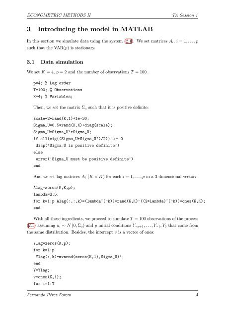
3 <strong>Intro</strong>ducing the model in <strong>MATLAB</strong><br />
In this section we simulate data using the system (2:1). We set matrices Ai, i = 1; : : : ; p<br />
such that the VAR(p) is stationary.<br />
3.1 Data simulation<br />
We set K = 4, p = 2 and the number of observations T = 100.<br />
p=4; % Lag-order<br />
T=100; % Observations<br />
K=4; % Variables;<br />
Then, we set the matrix u such that it is positive de…nite:<br />
scale=2*rand(K,1)+1e-30;<br />
Sigma_U=0.5*rand(K,K)+diag(scale);<br />
Sigma_U=Sigma_U’*Sigma_U;<br />
if all(eig((Sigma_U+Sigma_U’)/2)) >= 0<br />
disp(’Sigma_U is positive definite’)<br />
else<br />
error(’Sigma_U must be positive definite’)<br />
end<br />
And we set lag matrices Ai (K K) for each i = 1; : : : ; p in a 3-dimensional vector:<br />
Alag=zeros(K,K,p);<br />
lambda=2.5;<br />
for k=1:p Alag(:,:,k)=(lambda^(-k))*rand(K,K)-((2*lambda)^(-k))*ones(K,K);<br />
end<br />
With all these ingredients, we procced to simulate T = 100 observations of the process<br />
(2:1) assuming ut N (0; u) and p initial conditions Y p+1; : : : ; Y 1; Y0 that come from<br />
the same distribution. Besides, the intercept v is a vector of ones:<br />
Ylag=zeros(K,p);<br />
for k=1:p<br />
Ylag(:,k)=mvnrnd(zeros(K,1),Sigma_U)’;<br />
end<br />
Y=Ylag;<br />
v=ones(K,1);<br />
for i=1:T<br />
Fernando Pérez Forero 4