Cheat Perish? A Theory Scientific Customs

Filename: scientificmisbehavior-proofreading-dbspaceAC2.pdf December 1, 2016
now be rewritten as:
[
]
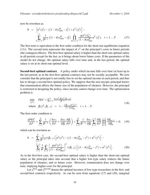
0 = u L (yt L ) − ((1 − π)y H min − yL t ) × u L′ (yt L ) −
T
∑
k=t+1
1 (
(1 − π)y
H
δ k−t min − y L ) k
k ∏
m=t+1
µu L (y L m)
(1 − π)u H u L′ (yt L ), t = 1...T. (17)
min
The first term is equivalent to the first-order condition for the short-run equilibrium (equation
(11)). The second term represents the impact of y L on the principal’s costs in future periods
(the contagion effects). The first-best optimal salary is higher than the short-run optimal salary
in all periods except for the last, as it brings about lower future costs. If the parameters of the
model do not change, the optimal salary falls over time and, in the last period, the optimal
salary is set at its short-run optimal level.
Second-best optimal contract. A policy under which income falls over time (at least up to
the last period, as in the first-best optimal contract) may not be socially acceptable. We now
consider that the principal is not totally free to set the optimal income in each period, and thus
has to design a second-best optimal policy. We suppose that the non-myopic principal knows
that remuneration affects the future size of the population of cheaters. However, the principal
is restricted in designing the policy, since income cannot change over time. The optimization
problem is
min
{y L }
PEC = ∑ T t=1
ec t (y L ,β t (y L ,β t−1 ))
δ t−1
where β t (y L ,β t−1 ) = 1 − v(β t−1)u L (y L )
, t = 1...T.
(1−π)u H min
(18)
The first-order condition is:
dPEC
dy L =
T
∑
t=1
which can be rewritten as:
0 =
T
∑
t=1
T −1
∑
t=1
(
1 ∂ect
δ t−1 ∂y L + ∂ec )
t ∂β t
∂β t ∂y L
+
T
∑
t=2
t−1
1 ∂ec t ∂β
δ t−1 ∂β t
∑
k
k=1
t−1
∂y ∏ L
m=k
1
[
]
δ t−1 v(β t−1) u L (y L ) − ((1 − π)y H min − yL ) × u L′ (y L ) −
[ µu L (y L )
1
δ t
t
∑
k=1
(1 − π)u H min
∂β m+1
∂β m
= 0, (19)
] k ]
v(β t−k )[
((1 − π)y H min − yL ) × u L′ (y L ) . (20)
As in the first-best case, the second-best optimal salary is higher than the short-run optimal
salary as the principal takes into account that a higher low-type salary reduces the future
population of cheaters, and so future costs. However, remuneration does not change over
time, implying higher costs for the principal.
Let yt
First and yt
Second denote the optimal incomes of low-type researchers in the first- and
second-best contracts respectively. As can be seen from equations (17) and (20), marginal
16