debtequity

(18). Thus there exists R ∗ > E(ã) such that Φ(α ∗ ; R ∗ ) = E(ã) and the Central Bank policy
(R B∗ , R D∗ ; α ∗ ) = (E(ã), R ∗ ; α ∗ ) leads to a Pareto optimal Flex equilibrium.
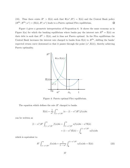
Figure 4 gives a geometric interpretation of Proposition 6. It shows the same economy as in
Figure 3(a) for which the banking equilibrium where banks pay the interest rate R B = E(ã) on
their debt is such that R E > E(ã), and is thus not Pareto optimal. In the Flex equilibrium the
Central Bank increases the interest rate charged to banks from E(ã) to R D∗ , shifting the banks’
expected return curve downward so that it passes through the point (α ∗ , E(ã)), thereby achieving
Pareto optimality.
Figure 4: Pareto optimal Flex equilibrium.
The equation which defines the rate R ∗ charged to banks
E(ã) = 1 ∫ ∞
α ∗ (a − (1 − α ∗ )R ∗ )f(a)da
(1−α ∗ )R ∗
can be written as
∫ ∞
(1 − α ∗ )R ∗ f(a)da =
(1−α ∗ )R ∗
∫ ∞
(1−α ∗ )R ∗ af(a)da − α ∗ E(ã)
= (1 − α ∗ )E(ã) −
which is equivalent to
∫ (1−α ∗ )R ∗
a
af(a)da
∫ ∞
R ∗ f(a)da + 1 ∫ (1−α ∗ )R ∗
(1−α ∗ )R ∗ 1 − α ∗ af(a)da = E(ã) (22)
a
37