n?u=RePEc:cep:cepdps:dp1458&r=bec

ISSN 2042-2695 

CEP Discussion Paper No 1458 

December 2016 

The Diffusion of Knowledge via Managers’ Mobility 

Giordano Mion 

Luca David Opromolla 

Alessandro Sforza

Abstract 

Better managers and managerial practices lead to better firm performance. Yet, little is known about what 

happens when managers move across firms. Does a firm hiring a good manager improve its performance? If yes 

is there some valuable knowledge the manager has acquired and successfully diffused to the new firm? In order 

to answer these questions, we use information related to specific activities the manager was involved in when 

working for previous firms. More specifically, we use information on whether the manager has worked in the 

past for firms exporting to a specific destination country or a specific product. Our data is rich enough to allow 

controlling for both manager and firm unobservables and wash out any time-invariant ability of the manager as 

well as overall firm performance. We find that the export experience gained by managers in previous firms leads 

their current firm towards higher export performance, and commands a sizable wage premium for the manager. 

We use several strategies to deal with endogeneity including an exogenous event study: the sudden end of the 

Angolan civil war in 2002. We further refine our analysis by looking at different types of managers (general, 

production, financial and sales) and show how specific export experience interacts with the degree of product 

differentiation and/or the financial vulnerability of a firm’s products as well as with rising import competition 

from China. 

Keywords: managers, knowledge diffusion, firm performance, job mobility, export experience 

JEL codes: M2; L2; F16; J31 

This paper was produced as part of the Centre’s Trade Programme. The Centre for Economic Performance is 

financed by the Economic and Social Research Council. 

Acknowledgements 

We thank seminar participants at various institutions and conferences for helpful comments. We also thank 

Lucena Vieira for computational assistance. The authors acknowledge financial support from Portuguese 

national funds by FCT (Fundação para a Ciência e a Tecnologia) project PTDC/EGE-ECO/122115/2010. This 

article is also part of the Strategic Project: PEst-OE/EGE/UI0436/2011. The opinion expressed are those of the 

authors and not necessarily those of Banco de Portugal. 

Giordano Mion, University of Sussex, Centre for Economic Performance, London School of 

Economics, CEPR and CESifo. Luca David Opromolla, Department of Economics, Bank of Portugal, CEPR and 

CESifo. Alessandro Sforza, Department of Geography and Environment, London School of Economics, and 

Centre for Economic Performance, London School of Economics. 

Published by 

Centre for Economic Performance 

London School of Economics and Political Science 

Houghton Street 

London WC2A 2AE 

All rights reserved. No part of this publication may be reproduced, stored in a retrieval system or transmitted in 

any form or by any means without the prior permission in writing of the publisher nor be issued to the public or 

circulated in any form other than that in which it is published. 

Requests for permission to reproduce any article or part of the Working Paper should be sent to the editor at the 

above address. 

© G. Mion, L. D. Opromolla and A. Sforza, submitted 2016.

1. Introduction 

“Managers are conductors of an input orchestra [...] Just as a poor conductor can lead 

to a cacophony rather than a symphony, one might expect poor management to lead to 

discordant production operations.” 

– Chad Syverson, What Determines Productivity (2011) 

The enormous variation in firm performance has become a focus of empirical and 

theoretical interest throughout the social sciences, including economics. Recent empirical 

studies have exploited the increasing availability of information on managerial practices 

and managers’ characteristics to establish a strong connection with firm—as well as 

country—productivity and other dimensions of performance. More specifically, Bloom 

and Van-Reenen (2010), Bloom et al. (2013), Bloom et al. (2016b) and Guiso and Rustichini 

(2011) among others, have established that better managers and managerial practices 

lead to better firm performance. We believe the next question is what happens when 

managers move from one firm to another. Does a firm hiring a good manager improve 

its performance? If yes is it due to the manager simply being a good manager or is there 

some valuable knowledge the manager has acquired and successfully diffused to the new 

firm? The objective of this paper is to provide answers to these questions. 

If sizeable knowledge diffusion happens via the mobility of managers we should, for 

example, expect that policies improving managerial practices in some firms will spill-over 

to other firms. In this respect, within the urban economics literature on spill-overs, there 

are some contributions showing how job hopping help sustain the competitiveness of 

local industry clusters like Silicon Valley. 1 Recent contributions to the international 

trade literature also highlight knowledge diffusion: 

Artopoulos et al. (2013) explain 

how the diffusion of business practices from export pioneers to followers can lead to 

sustained export growth, while Atkin et al. (2016) document a knowledge flow between 

intermediaries and foreign buyers leading to improvement in product quality. However, 

answering these questions is also difficult: First, it is challenging to separate a manager’s 

intrinsic capabilities from the knowledge and abilities she has learned in previous firms. 

Second, it is empirically difficult to show that such acquired knowledge and abilities 

impact current firm performance. 

In order to overcome the first challenge we draw on information related to specific activities 

the manager was involved in when working for previous firms. More specifically, 

we use information on whether the manager has worked in the past for firms exporting to 

1 Fallick et al. (2006) argue that job hopping is important in computer clusters because it facilitates 

the reallocation of talent and resources toward firms with superior innovations. Using detailed data on 

labor mobility, they find higher rates of job-hopping for college-educated men in Silicon Valley’s computer 

industry than in other computer clusters. 

1

a specific destination country or a specific product. Our data is rich enough to allow controlling 

for both manager and firm unobservables and wash out any time-invariant ability 

of the manager as well as overall firm performance. To tackle the second challenge we 

then relate this destination-specific or product-specific measure of acquired knowledge 

to the current firm trade performance in these specific destinations or products. In doing 

so we deal with the endogeneity of hiring in two complementary ways. First, we explore 

the differential performance of firms with and without managers with specific export 

experience in the wake of an exogenous event: the sudden end of the Angolan civil war 

in 2002. Second, we draw on the panel nature of the data and use information on whether 

the firm had managers with destination-specific or product-specific export experience 

3 years prior to evaluating firm-performance in those destinations or products. We 

further refine our analysis by looking at different types of managers (general, production, 

financial and sales) and show how specific export experience interacts with the degree of 

product differentiation and/or the financial vulnerability of a firm’s products as well as 

with rising import competition from China. 

We find that the export experience gained by managers in previous firms leads their 

current firm towards higher export performance, and commands a sizable wage premium 

for the manager. Moreover, export knowledge is decisive when it is market-specific: 

managers with experience related to markets (where by markets we mean destinations 

or products) served by their current firm receive an even higher wage premium; firms 

are more likely to enter markets where their managers have experience; exporters are 

more likely to stay in those markets, and their sales are on average higher. While it 

is reasonable to expect managers to learn valuable skills from their previous jobs and 

transfer them, the magnitudes we find are stark. Managers’ export experience is a 

first-order feature in the data explaining more variation in firm export performance than 

size and productivity. 

At the same time, we show that the experience premium accrued by different types 

of managers (general, production, financial and sales) aligns with a knowledge diffusion 

story. More specifically, we show that financial managers enjoy a basic export experience 

wage premium but no robust product- or destination-specific experience wage premium. 

General and production managers receive both a product- and a destination-specific experience 

premium but little or no basic experience premium. Sales managers benefit from 

a destination-specific experience premium while general managers get the largest premia 

in most cases. Furthermore, we find market-specific experience to be more valuable in 

terms of trade performance to firms selling products that are more differentiated and/or 

financially vulnerable while at the same time experience seems to help some firms coping 

with increasing import competition from China. 

Our analysis stands on three solid pillars: reliable data on one country (Portugal) 

2

covering the universe of firms and their workers for several years, including rich information 

on the characteristics of both; the possibility of tracking workers—and in 

particular managers—as they move from firm to firm; a research design that accounts 

for unobserved heterogeneity, omitted variables, and, more broadly, endogeneity. 

Our work relates to a number of strands in the literature. First, we contribute to the 

above cited empirical literature on management by showing how managers can diffuse 

knowledge and good practice across firms. Second, our work relates to the literature 

looking at the relationship between trade and tasks (Blinder, 2006, Grossman and Rossi- 

Hansberg, 2008). Such literature suggests that the complexity of the tasks involved in the 

different stages of production process (design, manufacturing of parts, assembly, R&D, 

marketing, commercialization, etc.) is key to understand recent trends in international 

trade. Managers are different from other workers and likely to be particularly important 

for trade activity because they are responsible for the most complex tasks within a firm. 

Third, the role played by managers’ mobility across firms in our analysis contributes to 

the recent debate about the channels via which knowledge diffusion takes place (Balsvik, 

2011, Parrotta and Pozzoli, 2012, Mion and Opromolla, 2014). 2 Last, but not least, 

our wage analysis contributes to the literature devoted to explaining the determinants 

of managers’ pay (Gabaix and Landier, 2008, Guadalupe and Wulf, 2008), and to the 

literature that studies the internal organization of the firm and how this relates to a firm’s 

characteristics such as export status (Caliendo and Rossi-Hansberg, 2012, Caliendo et al., 

2015). 

The remainder of the paper is organized as follows. Section 2 describes the data. In 

Section 3, after defining some key variables, we show raw data evidence positively associating 

a manager’s export experience with his/her wage and firm export performance. 

These descriptive results are confirmed by the econometric testing of Sections 4 and 5. 

Section 6 concludes and provides directions for further research. Additional details about 

the data are provided in the Appendix. The Tables Appendix provides complementary 

Tables. 

2. Data 

Our data combines information resulting from two panel datasets: 

international 

trade data at the firm-country-product level and matched employer-employee panel 

2 More specifically, we expand upon own research in Mion and Opromolla (2014) by considering 

different types of experience, different types of managers, the role of financial vulnerability and product 

differentiation as well as rising import competition from China. We also provide here further evidence 

on the causal impact of knowledge diffusion by exploring the differential performance of firms with and 

without managers with specific export experience in the wake of an exogenous event: the sudden end of 

the Angolan civil war in 2002. 

3

data. 

International trade data are collected by Statistics Portugal and—besides small 

adjustments—aggregate to the official total exports and imports of Portugal. 

For the 

purpose of this research, we use data on export transactions only, aggregated at the 

firm-destination-product-year level, for the period 1995-2005. 

Employer-employee data come from Quadros de Pessoal (henceforth, QP), a dataset 

collected by the Ministry of Employment, drawing on a compulsory annual census of all 

firms in Portugal that employ at least one worker. Reported data cover the firm itself, 

as well as each of its workers. 

Each firm and each worker entering the database are 

assigned a unique, time-invariant identifying number which we use to follow firms and 

workers over time. Currently, the data set collects data on about 350,000 firms and 3 

million employees. As for the trade data, we were able to gain access to information 

from 1995 to 2005. We describe the two datasets and their merging in more detail in the 

Appendix. 

The dataset allows to follow workers—especially managers—as they move from firm 

to firm; moreover, knowing firms’ trade status in each year, allows the identification 

of workers’ export experience. 

This is possible thanks to an exhaustive coverage of 

firms, their workers, and their trade activity as well as a high degree of reliability. The 

richness of the data also makes it possible to control for a wealth of both worker and firm 

characteristics as well as for unobserved heterogeneity by means of various fixed effects. 

We provide in the Appendix more information about the way we have constructed some 

of the covariates. 

We perform two complementary analyses. Because of our definitions of export experience, 

the analyses have been performed over the period 1996-2005. In Section 4, we 

estimate a wage equation to identify the existence of a wage premium for workers’—and 

in particular for managers’—export experience and its refinements: product and destination 

export experience. We subsequently show how premia are accrued by different types 

of managers (general, production, etc.) to further corroborate our story. In Section 5, we 

quantify the impact of the presence of managers with either destination or product export 

experience on a firm’s trade performance. At the end of that section, we strengthen the 

causal interpretation of our results by exploiting a natural experiment—the end of the 

civil war in Angola. We also show how export experience interacts with the degree of 

product differentiation and/or the financial vulnerability of a firm’s products 3 as well as 

3 The data on product differentiation comes from Rauch (1999) while data on financial vulnerability is 

taken from Manova et al. (2015). More specifically, we use for the former information on whether products 

are neither sold on an organized exchanged nor reference priced (liberal version) while for the latter we 

use the external financial dependence measure. 

4

Table 1: Selected Summary Statistics, Wage Sample, 2005 

Variable Mean Std. Dev. N 

Worker-level 

Hourly Wage (log) 1.351 0.518 436,351 

Age (Years) 38.206 10.695 436,351 

Education (Years) 7.449 3.586 436,351 

Tenure (Years) 10.043 9.277 436,351 

Manager (0/1) 0.067 0.250 436,351 

Manag. X Export Exp. (0/1) 0.015 0.122 436,351 

Manag. X Matched Dest. Export Exp. (0/1) 0.012 0.109 436,351 

Manag. X Matched Prod. Export Exp. (0/1) 0.011 0.104 436,351 

Current firm-level 

Firm Size (log) 2.339 1.142 25,681 

Firm Productivity (log) 10.480 0.908 25,681 

Firm Age (log) 2.461 0.816 25,681 

Foreign Ownership (0/1) 0.024 0.154 25,681 

At Least One Manag. (0/1) 0.274 0.446 25,681 

At Least One Manag. with Export Exp. (0/1) 0.083 0.276 25,681 

At Least One Manag. with Matched Dest. Export Exp. (0/1) 0.050 0.218 25,681 

At Least One Manag. with Matched Prod. Export Exp. (0/1) 0.046 0.209 25,681 

Previous firm-level 

Firm Size (log) 2.125 1.164 4,583 

Firm Productivity (log) 6.740 5.016 4,583 

Notes: This Table shows summary statistics, relative to 2005, for a subset of worker-level and firm-level variables used 

in the regressions of Section 4 and 5. Statistics refer to observations for which all covariates in the wage regression 

sample of Section 4 are jointly available. Firm-level variables subdivide into those relative to the worker’s current firm 

and to those relative to the previous firm. Variable names followed by "(0/1)" refer to dummy variables. In the last 

column, "N" refers to the number of workers for worker-level variables, and to the number of (current or previous) 

firms for firm-level variables. 

with rising competition due to Chinese imports. 4 In doing so we restrict the sample to 

firms with at least one employed manager. 5 Section 3 provides some raw data evidence 

that is consistent with the results of both analyses. 

4 We construct a measure of increase in Chinese import penetration that is both product and market 

specific along the lines of Autor et al. (2014). More specifically we consider the ratio between: (i) the 

change in the value of imports from China between 1995 and year t ∈ [1996, 2005] for a given Isic product 

in a given market; (ii) the value of apparent consumption (imports plus production minus exports) for 

a given Isic product in a given market and year t. We use the CEPII (Centre d’Etude Prospectives et 

d’Informations Internationales) trade and production dataset to compute such a measure. In our analysis 

a market is sometimes a group of countries and, when constructing apparent consumption for a given 

market, we do not consider imports and exports among countries belonging to the same market. 

5 The sample of firms is thus different in the two analyses; below we refer to the two sample as "wage 

sample" and "trade performance sample". The majority of firms in the wage sample lacks a (employed) 

manager. To identify managers in the data we need the person(s) running the firm to receive a wage: 

this can be a self-employed owner or a third person employed by the owner(s). Our trade performance 

analysis is thus representative of larger and more organizationally structured firms. Firms with at least 

one manager represent (in 2005) 53.6 percent of exporting firms, account for 91.8 percent of exports, and 

61.5 percent of employment of the Portuguese manufacturing industry. 

5

Table 1 reports summary statistics, for 2005, of the main worker-level and firm-level— 

both for the worker’s current and previous firm—variables used in our wage estimations 

and referring to observations for which all covariates are jointly available. The top panel 

of Table 1 indicates that, in 2005, our sample includes 436,351 workers, with an average 

(log) hourly wage of 1.35 euros, an average age of 38.2 years, an average education of 7.45 

years, and an average firm tenure of 10 years. 6 The middle panel of Table 1 shows that 

these workers are employed by 25,681 firms, and reports the average firm (log) size, (log) 

productivity, (log) age, and the share of foreign-owned firms (2.4 percent). Finally, the 

bottom panel provides the average (log) size and productivity of the 4,583 firms previously 

employing the workers in our sample. 

Table 2: Number of Exporters and Average Exports, by Country-group, Trade Sample, 2005 

Markets 

IT-UK Other Other 

Variable Spain FR-DE EU OECD CPLP China ROW 

# of Exporting firms 1,696 1,711 1,285 1,401 1,097 204 1,227 

—with Export Exp. 838 833 644 711 558 127 651 

—with Matched Dest. Export Exp. 717 736 524 624 455 57 547 

Avg. Exports 2,322 4,046 1,454 1,244 301 596 950 

Notes: This Table shows the number of firms exporting to each of the seven markets we consider and their average exports (in 

thousands euros) for the 2005 sample year. The number of exporters further subdivides into those having at least one manager 

with export experience and those having at least one manager with matched (destination) export experience. Statistics refers 

to observations for which all covariates in the trade performance analysis sample of Section 5 are jointly available. CPLP is the 

Portuguese acronym for the Community of Portuguese Language Countries. 

Tables 2 and 3 report selected summary statistics—for 2005—referring to the trade 

performance sample. In Section 5 we model a firm’s entry and continuation into a specific 

destination, or into a specific product market, m, and analyze both the probability to start 

and continue exporting as well as the value of exports conditional on entry/continuation. 

When considering destinations, we partition countries into seven groups: Spain (the 

most frequent destination), other top 5 export destination countries (Italy, UK, France, 

and Germany), other EU countries, OECD countries not belonging to the EU, countries 

belonging to the Community of Portuguese Language Countries (CPLP in Portuguese), 

China, and the rest of the World. Table 2 shows, for each of the seven destinations, the 

number of exporting firms and average exports (in thousand euros). When considering 

products, we partition markets into 29 Isic rev.2 groups. The largest groups, in terms 

of total exports, are 384 "Transport equipment", 383 "Electrical machinery apparatus, 

6 Carneiro et al. (2012) find that average (log) hourly earnings (in real Euros) are 1.34 for men and 1.13 

for women, in the 1986-2005 period. Workers’ tenure and wage are described in the Appendix. 

6

Table 3: Number of Exporters and Average Exports, Seven largest product groups, Trade Sample, 2005 

Markets 

Textiles Wearing Paper Industrial Machinery Electrical Transport 

Variable apparel products chemicals exc. electrical machinery equipment 

# of Exporting firms 515 508 316 368 739 324 228 

—with Export Exp. 272 205 195 225 393 187 143 

—with Matched Prod. Export Exp. 194 149 122 152 327 135 92 

Avg. Exports 1,940 2,125 2,813 2,593 2,389 5,779 10,940 

Notes: This Table shows the number of firms exporting to each of the seven largest, in terms of total exports, product groups in our sample, 

and their average exports (in thousands euros) for the 2005 sample year. The number of exporters further subdivides into those having at 

least one manager with export experience and those having at least one manager with matched (product) export experience. Statistics refers to 

observations for which all covariates in the trade performance analysis sample of Section 5 are jointly available. The number and full titles of the 

product groups are 384 "Transport equipment", 383 "Electrical machinery apparatus, appliances and supplies" 382 "Machinery except electrical" 

322 "Wearing apparel, except footwear" 321 "Textiles" 351 "Industrial chemicals", and 341 "Paper and paper products". See the Appendix for 

details on the product definition. 

appliances and supplies" 382 "Machinery except electrical" 322 "Wearing apparel, except 

footwear" 321 "Textiles" 351 "Industrial chemicals", and 341 "Paper and paper products" 

Table 3 shows, for each of the seven largest product groups, the number of exporting 

firms and average exports (in thousand euros). 

3. Main definitions and evidence from raw data 

In this Section we draw the distinction between managers and non-managers, we define 

export experience as well as its two refinements: experience in a destination and 

experience in a product. We also show raw data evidence on the existence of an export 

experience wage premium for managers, and on the impact of managers with export 

experience on a firm’s trade performance. 

3.1 Managers 

In our analysis, we partion workers into managers and non-managers. As it is effectively 

captured by the quote of Syverson (2011) at the beginning of the paper, managers are 

responsible for strategic decisions taken within the firm including the organization of 

the firm, planning, and the shaping of technical, scientific and administrative methods 

7

or processes. 7 

In practice, we identify managers using a (compulsory) classification of workers, 

according to eight hierarchical levels, defined by the Portuguese law (Decreto Lei 121/78 

of July 2 nd 1978). Classification is based on the tasks performed and skill requirements, 

and each level can be considered as a layer in a hierarchy defined in terms of increasing 

responsibility and task complexity. Managers are defined as the workers belonging to 

one of the top two hierarchical levels: “Top management” and “Middle management”; 

non-manager are workers belonging to lower hierarchical levels. Table 1 shows that, in 

the wage sample in 2005, 6.7 percent of the workers are managers and 27.4 percent of the 

firms have at least one manager. 

We then take a deeper look into the professional status of the manager by analysing 

the exact occupation within a firm. Using the four digit ISCO classification in Quadros 

de Pessoal, we look at the professional status of the managers specifically focusing on 

directors, the category to which the vast majority of managers belong to. We end up 

with 4 groups: general managers, production managers, financial managers and sales 

managers. 

managers). 

We lump managers covering other occupations into a fifth group (other 

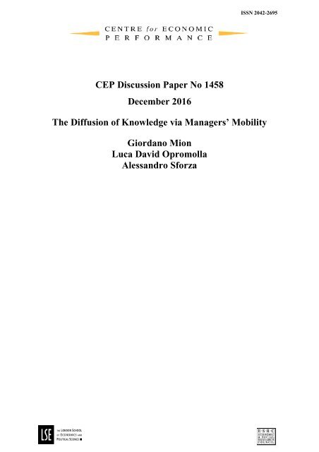
Figure 1 confirms that the distinction between managers and non-managers is relevant 

when considering a firm’s trade activity. 

A large literature tries to identify and 

explain a wage premium paid by exporting firms (Frias et al., 2009, Munch and Skaksen, 

2008, Schank et al., 2007). Martins and Opromolla (2012), show that Portugal is not 

an exception to this robust empirical finding. Figure 1 shows that the exporter wage 

premium seems to come essentially from managers. More specifically, Figure 1 shows 

the kernel density of the log hourly wage distribution in our 2005 wage sample, both 

for managers and non-managers, broken down by firm export status (exporters and 

non-exporters). The wage density referring to managers employed by exporting firms 

clearly lies to the right of the one for managers employed by non-exporters. The evidence 

7 The distinction between managers and non-managers is relevant in light of recent developments in the 

international trade literature: Antràs et al. (2006) and Caliendo and Rossi-Hansberg (2012) explicitly focus 

on the formation of teams of workers in a globalized economy, and emphasize that the key distinction 

between managers and non-managers is that the former are in charge of complex tasks. Managers are 

different from other workers because they are responsible for the most complex tasks—those that are 

crucial for international trade performance—within a firm. Second, managers are “special” when it comes 

to doing business in foreign markets because they are in charge of marketing and commercialization 

activities (which are not necessarily more complex) such as, for example, setting-up distribution channels, 

finding and establishing relationships with foreign suppliers, setting up marketing activities directed at 

finding and informing new buyers, and building a customer base. Arkolakis (2010) and Eaton et al. 

(2015) stress the key role of search and marketing costs in international trade and provide evidence of the 

importance of the continuous “search and learning about foreign demand” problem that firms face when 

selling abroad. At the same time, Araujo et al. (2016) show the importance of trust-building in repeated 

interactions between sellers and buyers in an international market. 

8

Figure 1: Wage density for managers and non-managers, by firm export status, 2005 

Managers 

Non−managers 

Density 

0 .2 .4 .6 .8 1 

Density 

0 .2 .4 .6 .8 1 1.2 1.4 1.6 1.8 2 

.5 1 1.5 2 2.5 3 3.5 

(Log) Wage 

Nonexporters 

.5 1 1.5 2 2.5 3 3.5 

(Log) Wage 

Exporters 

Notes: This Figure shows the kernel density of the (log) hourly wage distribution in 2005 for managers (left panel) and nonmanagers 

(right panel), broken down by firm export status (exporters and non-exporters). Statistics refers to observations for which 

all covariates in the wage regression sample of Section 4 are jointly available. The kernel is Epanechnikov and the kernel width is the 

Stata default one. 

for non-managers is instead much weaker. 

3.2 Export experience 

Managers are not all alike: their set of skills and knowledge can be tightly connected to 

the experience they faced along their careers. In particular, only some managers have 

the chance to be involved in export activities. To the extent that experience acquired in 

exporting firms substantially improves the capacities and skills of a manager it should 

correspond to a wage premium. Furthermore, such experience is potentially valuable to 

all firms, but in particular to exporters, who might expect an improvement of their trade 

performance. 

We exploit the matched employer-employee feature of our dataset to track workers 

over time: for each firm-year pair, we identify the subset of (currently employed) workers 

that have previously worked in a different firm. Moreover, we exploit the trade dataset to 

single-out those workers that were employed in the past by an exporting firm. We define 

such workers, and in particular managers, as having export experience. 8 

8 Table 1 indicates that about 23 percent of the managers (0.015/0.067) have export experience, while 8.3 

percent of firms—i.e. 30% of the firms with at least one manager—have at least one manager with export 

experience. 

9

To gain further insights we consider in our framework two related refinements of 

export experience. The first refinement is market specific export experience, where a 

market indicates either a destination d or a product p. The former refers to one of the 

seven markets listed in Section 2 while the latter to one of the 29 product groups defined 

using the Isic rev2 classification (see the Appendix). We define a worker as having 

destination d-specific export experience if he/she has export experience and destination 

d was among the destinations served by one of the worker’s previous employers during 

the period of time the worker was employed there. Symmetrically, we define a worker as 

having product p-specific export experience if he/she has export experience and product 

p was among the product exported by one of the worker’s previous employers during the 

period of time the worker was employed there. The second refinement is matched export 

experience. We define a worker as having matched export experience in a destination if 

he/she has export experience and has market d-specific export experience in at least one 

of the markets to which the current employing firm is actually exporting. Moreover, a 

worker can have matched export experience in a product group when he/she has export 

experience and has product p-specific export experience in at least one of the products 

the current employing firm is actually exporting. 

Figures 2 to 5 provide raw wage data evidence supporting the idea that the distinction 

between managers with and without export experience is relevant when considering a 

firm’s international activity. Furthermore they also highlight the importance of destination 

and product experience. More specifically Figures 2 and 3 show the wage density for 

managers with export experience dominates the one corresponding to managers without 

experience. At the same time, Figure 2 (3) suggests the presence of an additional wage 

premium for destination-specific (product-specific) matched export experience over basic 

experience. Furthermore, Figures 4 and 5 indicate the above holds for all of the five 

categories of managers we consider. 

3.3 Export experience and trade performance 

Figures 6 to 9 analyze more directly the correlation between the presence of managers 

with experience in a firm and that firm’s export performance. More specifically they 

focus on two export performance margins, namely the probability to start and probability 

to continue exporting in a given destination d (Figures 6 and 7) or a given product p 

(Figures 8 and 9). We consider three categories of firms: those without managers with 

export experience, those with at least one manager with export experience, and those 

with at least one manager with specific (destination or product) export experience. It 

can be readily appreciated that in all instances the presence of managers with export 

experience within a firm is associated to a higher probability to start/continue exporting 

10

while at the same time having at least one manager with specific export experience is 

associated with an even higher probability. This is by no means a proof of causality but 

certainly a strong feature of the data one needs to address. 

Figure 2: Wage density for managers by export experience in a destination, 2005 

Density 

0 .2 .4 .6 .8 1 

.5 1 1.5 2 2.5 3 3.5 

(Log) Wage 

Without Export Experience 

With Matched−Destination Export Experience 

With Export Experience 

Notes: This Figure shows the kernel density of the (log) hourly wage distribution in 2005 for managers, broken down by degree of 

export experience (in a destination). Statistics refers to observations for which all covariates in the wage regression sample of Section 

4 are jointly available. The kernel is Epanechnikov and the kernel width is the Stata default one. 

11

Figure 3: Wage density for managers by export experience in a product, 2005 

Density 

0 .2 .4 .6 .8 1 

.5 1 1.5 2 2.5 3 3.5 

(Log) Wage 


With Matched−Product Export Experience 


Notes: This Figure shows the kernel density of the (log) hourly wage distribution in 2005 for managers, broken down by degree of 

export experience (in a product). Statistics refers to observations for which all covariates in the wage regression sample of Section 4 

are jointly available. The kernel is Epanechnikov and the kernel width is the Stata default one. 

Figure 4: Wage density of managers distinguishing by: manager type and export experience (in 

a destination), 2005 

Other manager 

General manager 

Production manager 

Density 

0 .2 .4 .6 .8 1 

Density 

0 .2 .4 .6 .8 1 

Density 

0 .2 .4 .6 .8 1 

.5 1 1.5 2 2.5 3 3.5 

(Log) Wage 

Financial manager 

.5 1 1.5 2 2.5 3 3.5 

(Log) Wage 

Sales manager 

.5 1 1.5 2 2.5 3 3.5 

(Log) Wage 

Density 

0 .2 .4 .6 .8 1 

Density 

0 .2 .4 .6 .8 1 

.5 1 1.5 2 2.5 3 3.5 

(Log) Wage 

.5 1 1.5 2 2.5 3 3.5 

(Log) Wage 


With Matched−Destination Export Experience 


Notes: This Figure shows the kernel density of the (log) hourly wage distribution in 2005 for managers, broken down by manager 

type and degree of export experience (in a destination). Statistics refers to observations for which all covariates in the wage regression 

sample of Section 4 are jointly available. The kernel is Epanechnikov and the kernel width is the Stata default one. 

12

Figure 5: Wage density of managers distinguishing by: manager type and export experience (in 

a product), 2005 

Other manager 

General manager 

Production manager 

Density 

0 .2 .4 .6 .8 1 

Density 

0 .2 .4 .6 .8 1 

Density 

0 .2 .4 .6 .8 1 

.5 1 1.5 2 2.5 3 3.5 

(Log) Wage 

Financial manager 

.5 1 1.5 2 2.5 3 3.5 

(Log) Wage 

Sales manager 

.5 1 1.5 2 2.5 3 3.5 

(Log) Wage 

Density 

0 .2 .4 .6 .8 1 

Density 

0 .2 .4 .6 .8 1 

.5 1 1.5 2 2.5 3 3.5 

(Log) Wage 

.5 1 1.5 2 2.5 3 3.5 

(Log) Wage 


With Matched−Product Export Experience 


Notes: This Figure shows the kernel density of the (log) hourly wage distribution in 2005 for managers, broken down by manager 

type and degree of export experience (in a product). Statistics refers to observations for which all covariates in the wage regression 

sample of Section 4 are jointly available. The kernel is Epanechnikov and the kernel width is the Stata default one. 

Figure 6: Export entry rate, experience in a destination, 2005 

0 .02 .04 .06 .08 .1 

Spain 

IT−UK−FR−DE 

Other EU 

Other OECD 

CPLP 

China 

Rest of the World 

No Export Experience 

Specific Export Experience 

Export Experience 

Notes: This Figure shows entry rates, defined as the ratio between the number of firms starting to export in destination d at time 

t and the number of firms not exporting to destination d at time t-1, for each destination in 2005, for three groups of firms: those 

that have no managers with export experience at time t, those that have at least one manager with export experience at time t, and 

those that have at least one manager with specific export experience at time t. CPLP is the Portuguese acronym for the Community 

of Portuguese Language Countries. 

13

Figure 7: Export continuation rate, experience in a destination, 2005 

0 .2 .4 .6 .8 1 

Spain 

IT−UK−FR−DE 

Other EU 

Other OECD 

CPLP 

China 

Rest of the World 


Specific Export Experience 


Notes: This Figure shows continuation rates, defined as the share of firms continuing to export to destination d at time t among those 

firms that were already exporting to destination d at time t, for each destination in 2005, for three groups of firms: those that have no 

managers with export experience at time t, those that have at least one manager with export experience at time t, and those that have 

at least one manager with specific export experience at time t. CPLP is the Portuguese acronym for the Community of Portuguese 

Language Countries. 

Figure 8: Export entry rate density, experience in a product, 2005 

Density 

0 50 100 150 

0 .03 .06 .09 .12 

Entry Rate 


Specific−Product Export Experience 


Notes: This Figure shows kernel densities for entry rates, defined as the ratio between the number of firms starting to export product 

p at time t and the number of firms not exporting product p at time t-1, for each product in 2005, for three groups of firms: those 

that have no managers with export experience at time t, those that have at least one manager with export experience at time t, and 

those that have at least one manager with specific export experience at time t. The kernel is Epanechnikov and the kernel width is 

the Stata default one. 

14

Figure 9: Export continuation rate density, experience in a product, 2005 

Density 

0 2 4 

0 .2 .4 .6 .8 1 

Continuation Rate 


Specific−Product Export Experience 


Notes: This Figure shows kernel densities for continuation rates, defined as the share of firms continuing to export product p at time 

t among those firms that were already exporting product p at time t, for each product in 2005, for three groups of firms: those that 

have no managers with export experience at time t, those that have at least one manager with export experience at time t, and those 

that have at least one manager with specific export experience at time t. The kernel is Epanechnikov and the kernel width is the Stata 

default one. 

4. Wage analysis 

The first step towards establishing a relationship between the export experience brought 

by managers into a firm and the firm’s trade performance consists in assessing whether 

export experience corresponds to a wage premium. In this Section, we estimate a 

Mincerian wage equation to show that managers with export experience (as defined 

in Section 3) enjoy a sizeable wage premium. The premium is robust to controlling for 

worker and firm fixed effects, previous firm observables, job-change patterns, as well as a 

large set of worker and current firm time-varying observables. Moreover, managers with 

experience in one (or more) of the current destinations reached or products exported 

by their firm—i.e. matched destination- or product-specific export experience—enjoy 

an even higher wage premium. 9 These results confirm previous evidence in Mion and 

Opromolla (2014) for destination-specific experience and paint a new but similar portrait 

for product-specific experience. 

9 See Section 3 for the definition of specific export experience. 

15

We further enrich the analysis by looking at the experience premia accrued by different 

types of managers (general, production, financial and sales) and find results in line 

with a knowledge diffusion story. More specifically, we show that financial managers 

enjoy a basic export experience premium but no robust product- or destination-specific 

experience premium. General and production managers receive both a product- and 

a destination-specific experience premium but little or no basic experience premium. 

Sales managers benefit from a destination-specific experience premium while general 

managers get the largest premia in most cases. Crucially, we find little evidence of a 

wage premium for non-managers, which is the reason why in the trade performance 

analysis of Section 5 we focus on managers only. These results add the evidence coming 

from raw wage data shown in the previous Section. 

There are caveats in our analysis as well as alternative explanations for the existence 

of a premium that do not involve the diffusion of valuable export-specific knowledge by 

managers. Though, such alternative explanations are at odds with the existence of an 

additional wage premium for specific export experience and, as we will show later on, 

potentially imply our premia are actually under-estimated. We discuss these issues in 

more detail in Section 4.3. 

4.1 Econometric model 

Workers are indexed by i, current employing firms by f, previous employing firms by p, 

and time by t. Each worker i is associated at time t to a unique current employing firm 

f and a unique previous employing firm p. The baseline wage equation we estimate is: 

w it = β 0 + β 1 Manager it + Mobility ′ it Γ M + (Mobility it × Manager it ) ′ Γ Mm + 

+β 2 Experience it + β 3 (Experience it × Manager it ) + 

+β 4 Matched_Experience it + β 5 (Matched_Experience it × Manager it ) + 

(1) 

+I ′ it Γ I + P ′ pt Γ P + C ′ ft Γ C + η i + η f + η t + ε it , 

where w it is the (log) hourly wage of worker i in year t, Manager it is a dummy indicating 

whether worker i is a manager at time t, the vector Mobility it contains a set of dummies 

taking value one from the year t a worker changes employer for the 1 st , 2 nd ,..time, 

Experience it and Matched_Experience it are dummies indicating whether worker i has, 

respectively, export experience and matched (destination or product; we estimate two 

separate regressions) export experience at time t, the vector I it stands for worker i 

16

time-varying observables, 10 the vectors P pt and C ft refer to, respectively, the previous 

and current employing firm observables, 11 η i (η f ) are individual (firm) fixed effects and 

η t are time dummies. 

The key parameters in our analysis are β 2 + β 3 , i.e., the wage premium corresponding 

to export experience for a manager, and β 4 + β 5 , i.e., the extra premium corresponding to 

matched export experience for a manager. β 2 and β 4 indicate, respectively, the premium 

related to export experience and matched export experience for a non-manager. Mobility 

of workers across firms is needed, according to our definition, to acquire export experience: 

Experience it =1 if worker i has, among his/her previous employers, an exporting 

firm while Matched_Experience it =1 further requires the current employing firm to be 

exporting: (i) one or more of the products previous employers were exporting (experience 

in a product regressions); (ii) in at least one of the markets to which previous employers 

were exporting (experience in a destination regressions). In other words, identification of 

export experience premia comes from workers moving across firms. To disentangle wage 

variations due to mobility from those related to export experience we consider the set of 

dummies Mobility it . We further interact Mobility it with manager status Manager it to 

allow mobility to have a differential impact on managers and non-managers. 

Mobility it , Experience it , and Matched_Experience it , as well as their interaction with 

manager status, thus define a difference-in-difference setting with two treatments (acquiring 

export experience and eventually also matched export experience) and a control 

group of workers (managers and non-managers) changing employer without acquiring 

export experience. 12 

Equation (1) is first estimated without worker and firm fixed effects, then with firm 

fixed effects and finally with both sets of fixed effects. In all three cases we consider 

two specifications: with export experience only and with both export experience and 

10 A worker’s age, age squared, education, and tenure. See Section 2 and the Appendix for further 

details. 

11 Previous firm observables are size, productivity, and a dummy indicating whether the current and 

previous firms belong to the same industry or not. Current firm observables are size, productivity, share 

of skilled workers, export status, age, foreign ownership, mean and standard deviation of both age and 

education of managers, and industry-level exports. For previous firm variables, as well as for current 

firm variables requiring knowledge of managers’ age and education, we add a set of dummies equal to 

one whenever the data are missing, while recoding missing values to zero. Previous employing firm 

information is not available for workers who enter the labor market in our time frame or workers who 

always stay in the same firm. We do this to maximize exploitable information. When we then turn to the 

trade performance analysis which is, as detailed above, representative of larger and more organizationally 

structured firms we simply discard missing observations. We consider both manufacturing and nonmanufacturing 

firms in constructing previous employing firm variables. In specifications without fixed 

effects we add NUTS3 location and Nace rev.1 2-digit dummies as further controls. See Section 2 and the 

Appendix for further details. 

12 Our regression design is likely to actually underestimate the value of export experience. For example, 

mobility dummies would absorb some of the effect of the export-related learning to the extent greater 

knowledge leads managers to receive more job offers and hence move around more. 

17

matched export experience. As already indicated we present separate regressions Tables 

for experience in a destination and experience in a product. Last but least when focusing 

on the different types of managers we break down the Manager it dummy (and its 

interactions with experience) into 5 categories (general, production, financial, sales and 

other). All our specifications are estimated with OLS and we deal high-dimensional fixed 

effects building on the full Gauss-Seidel algorithm proposed by Guimarães and Portugal 

(2010). See the Appendix for further details. 

4.2 Results 

Table 4 and 5 report the estimated export experience premia obtained from the different 

variants of (1) both for manager and non-managers. More specifically in Table 4 we 

consider wage regressions with basic experience and experience in a destination while in 

Table 5 we consider wage regressions with basic experience and experience in a product. 

The two Tables also show the significance levels of the premia, along with values of the 

F-statistics for managers’ premia and T-statistics for non-managers’ premia. 13 Tables B-15 

to B-20 in the Tables Appendix provide information on all the other covariates. Such 

Tables show that coefficient signs and magnitudes are in line with previous research 

based on Mincerian wage regressions, i.e., wages are: higher for managers, increasing 

and concave in age, increasing in education and tenure, higher in larger, more productive, 

foreign-owned and older firms, higher in firms with a larger share of skilled workers. 

The overall picture coming out from Tables 4 and 5 can be summarized as follows: 

Export experience does pay for a manager. Columns (1) to (3) in the two Tables 14 point to 

a premium in between 11.5% (no fixed effects) and 2.7% (worker and firm fixed effects). 

The latter figure should be considered as extremely conservative because, due to the 

presence of worker fixed effects, we are identifying that coefficient from workers who 

are currently managers but were not managers in the past. Yet the 2.7% is economically 

big representing about half of the premium (5.8%) for being a manager in the estimation 

corresponding to column 3. 

At the same time the difference in the premium across 

specifications do suggest that managers with export experience are “better managers” 

and work for better paying firms. However, a premium remains when controlling for 

both firm and worker time-invariant heterogeneity indicating that export experience 

13 Managers’ premia are obtained from sums of covariates’ coefficients in equation (1). Therefore, 

their significance is tested with an F-statistic. Non-managers’ premia correspond instead to individual 

coefficients in equation (1) and so the T-statistic is used. 

14 Note results are identical between the two Tables and rightly so. 

18

Table 4: Wage regression with basic experience and experience in a destination 

Controls (1) (2) (3) (4) (5) (6) 

Export Experience Premia for Managers 

Export Experience 0.115 a 0.110 a 0.027 a 0.064 a 0.042 a 0.013 c 

(870.8) (859.3) (27.4) (103.4) (50.3) (3.5) 

Destination-Specific Exp. Experience 0.061 a 0.089 a 0.017 a 

(100.3) (230.1) (9.7) 

Export Experience Premia for non-Managers 

Export Experience 0.006 a 0.014 a -0.003 c 0.022 a 0.010 a -0.003 

(7.6) (17.0) (-1.7) (21.8) (10.6) (-1.1) 

Destination-Specific Exp. Experience -0.028 a 0.007 a -0.003 

(-25.4) (6.5) (-1.0) 

Observations 4,006,826 4,006,826 4,006,826 4,006,826 4,006,826 4,006,826 

R 2 0.598 0.697 0.925 0.598 0.697 0.925 

Worker controls X X X X X X 

Firm (current and past) controls X X X X X X 

Firm FE X X X X 

Worker FE X X 

Notes: This Table reports export experience premia from the OLS estimation of several variants of the mincerian 

wage equation (1). The dependent variable is a worker’s (log) hourly wage in euros. Export experience and 

matched (destination) export experience are dummies. See Section 3 for the definition of a manager and the export 

experience (and its refinements). Estimations include a number of covariates whose coefficients and standard errors 

are reported in the Tables Appendix. Worker-year covariates include a worker’s age, age square, education, and 

tenure. Current firm-time covariates include firm size, productivity, share of skilled workers, export status, age, 

foreign ownership, mean and standard deviation of both age and education of managers, and industry-level exports. 

Previous firm-time covariates include firm size, productivity, and a dummy indicating whether current and previous 

employing firms industry affiliations coincide or not. See the Appendix for details on covariates. All specifications 

include year dummies, and those not including fixed effects also contain region (NUTS-3) and industry (NACE 

2-digits) dummies. Robust F-statistics (t-statistics) for managers (non-managers) premia in parentheses: a p < 0.01, 

b p < 0.05, c p < 0.1. 

is not simply a proxy for managers’ unobserved ability and/or selection into higher 

paying firms. Export experience is neither a trivial proxy for, as an example, a stronger 

bargaining position of a manager moving out of a successful/productive firm. We do 

control, in all specifications, for the size, productivity, and industry affiliation of the 

manager’s previous firm. As shown in Tables B-15 to B-20 in the Tables Appendix 

managers that come from more productive firms do earn a higher wage, but export 

experience continues to be positively and significantly associated to a wage premium for 

managers. 

There is an additional premium for matched export experience for managers. Columns (4) to 

(6) in Table 4 point to an additional premium accrued upon having destination-specific 

experience, with respect to just having basic experience, in between 8.9% (firm fixed 

effects) and 1.7% (worker and firm fixed effects). The corresponding figures for the 

product-specific experience premium are 10% and 0.7% even though the latter fails to be 

significant. Overall our findings suggest specific experience is an important feature of a 

19

Table 5: Wage regression with basic experience and experience in a product 

Controls (1) (2) (3) (4) (5) (6) 

Export Experience Premia for Managers 

Export Experience 0.115 a 0.110 a 0.027 a 0.072 a 0.046 a 0.022 a 

(870.8) (859.3) (27.4) (182.9) (79.0) (12.4) 

Product-Specific Exp. Experience 0.061 a 0.100 a 0.007 

(127.1) (360.9) (1.7) 

Export Experience Premia for non-Managers 

Export Experience 0.006 a 0.014 a -0.003 c 0.013 a 0.003 a -0.008 a 

(7.6) (17.0) (-1.7) (13.0) (2.9) (-3.5) 

Product-Specific Exp. Experience -0.012 a 0.025 a 0.006 a 

(-11.4) (22.7) (4.8) 

Observations 4,006,826 4,006,826 4,006,826 4,006,826 4,006,826 4,006,826 

R 2 0.598 0.697 0.925 0.598 0.697 0.925 




Worker FE X X 

Notes: This Table reports export experience premia from the OLS estimation of several variants of the mincerian 

wage equation (1). The dependent variable is a worker’s (log) hourly wage in euros. Export experience and 

matched (product) export experience are dummies. See Section 3 for the definition of a manager and the 

export experience (and its refinements). Estimations include a number of covariates whose coefficients and 

standard errors are reported in the Tables Appendix. Worker-year covariates include a worker’s age, age square, 

education, and tenure. Current firm-time covariates include firm size, productivity, share of skilled workers, 

export status, age, foreign ownership, mean and standard deviation of both age and education of managers, and 

industry-level exports. Previous firm-time covariates include firm size, productivity, and a dummy indicating 

whether current and previous employing firms industry affiliations coincide or not. See the Appendix for details 

on covariates. All specifications include year dummies, and those not including fixed effects also contain region 

(NUTS-3) and industry (NACE 2-digits) dummies. Robust F-statistics (t-statistics) for managers (non-managers) 

premia in parentheses: a p < 0.01, b p < 0.05, c p < 0.1. 

manager’s wage and are consistent with the hypothesis that managers diffuse valuable 

export-related knowledge. While the existence of a premium for export experience is also 

consistent with the diffusion of knowledge not uniquely related to exporting (e.g. R&D 

skills, organizational practices, etc.) the additional premium for matched experience 

does reinforce the view that export-specific knowledge is an important component of 

the knowledge diffusion. Furthermore, our results suggest that such knowledge proves 

to be very valuable when it is market-specific (product or destination). 

There is limited evidence that export experience pays for non-managers. Non-managers 

premia across Tables 4 and 5 are substantially smaller than those corresponding to 

managers and less often significant. Given the key role of managers for export-specific 

activities, the weaker evidence for premia among non-managers is consistent with 

export experience entailing some valuable export-specific knowledge. Managers are 

“special” because exporting requires successfully performing a number of complex 

tasks and managers are the employees that are responsible for the most sophisticated 

20

tasks within a firm (e.g. Antràs et al., 2006, Caliendo and Rossi-Hansberg, 2012). 

Furthermore, managers are also different because they are in charge of marketing and 

commercialization activities. As suggested by Arkolakis (2010) and Eaton et al. (2015), 

searching for customers and suppliers and learning about their needs play a key role in 

determining the success of a firm on the international market. 

Table 6: Wage regression with different types of managers and export experience 

Controls (1) (2) (3) (4) (5) (6) 



General manager 0.078 a 0.072 a -0.001 0.116 a 0.110 a 0.020 

(13.1) (12.9) (0.0) (29.1) (30.5) (1.2) 

Production manager 0.053 a 0.049 a 0.018 0.041 a 0.047 a 0.025 b 

(11.2) (10.9) (1.5) (8.3) (12.1) (4.1) 

Financial manager 0.056 a 0.033 c 0.092 a 0.101 a 0.090 a 0.084 a 

(7.5) (3.0) (10.6) (28.4) (23.0) (13.4) 

Sales manager -0.030 -0.024 a 0.012 0.021 0.031 0.042 c 

(1.4) (1.1) (0.2) (1.0) (2.4) (3.3) 

Destination-Specific Exp. Experience 

Product-Specific Exp. Experience 

General manager 0.482 a 0.428 a 0.091 a 0.432 a 0.385 a 0.058 a 

(298.1) (262.8) (15.4) (231.7) (208.7) (6.8) 

Production manager 0.132 a 0.158 a 0.036 b 0.169 a 0.184 a 0.026 c 

(56.1) (86.4) (5.4) (105.1) (132.7) (3.5) 

Financial manager 0.156 a 0.190 a -0.015 0.110 a 0.134 a -0.006 

(45.2) (73.7) (0.2) (24.8) (37.5) (0.8) 

Sales manager 0.212 a 0.221 a 0.039 c 0.164 a 0.173 a 0.000 

(59.6) (76.6) (3.0) (44.0) (55.7) (0.0) 

Observations 4,006,826 4,006,826 4,006,826 4,006,826 4,006,826 4,006,826 

R 2 0.599 0.698 0.925 0.599 0.698 0.925 




Worker FE X X 

Notes: This Table reports export experience premia from the OLS estimation of several variants of the mincerian wage 

equation (1). The dependent variable is a worker’s (log) hourly wage in euros. In specifications (1) to (3) both export 

experience and destination-specific export experience are considered along with their interactions with dummies 

corresponding to different types of managers. In specifications (4) to (6) both export experience and product-specific 

export experience are considered along with their interactions with dummies corresponding to different types of 

managers. See Section 3 for the definition of a manager, manager types and for export experience (and its refinements). 

Estimations include a number of covariates whose coefficients and standard errors are reported in the Tables Appendix. 

Worker-year covariates include a worker’s age, age square, education, and tenure. Current firm-time covariates 

include firm size, productivity, share of skilled workers, export status, age, foreign ownership, mean and standard 

deviation of both age and education of managers, and industry-level exports. Previous firm-time covariates include 

firm size, productivity, and a dummy indicating whether current and previous employing firms industry affiliations 

coincide or not. See the Appendix for details on covariates. All specifications include year dummies, and those not 

including fixed effects also contain region (NUTS-3) and industry (NACE 2-digits) dummies. Robust F-statistics in 

parentheses: a p < 0.01, b p < 0.05, c p < 0.1. 

Table 6 provides additional insights into the nature of export experience premia. More 

specifically, we now split managers into several categories depending on their specific 

21

ole within a firm and compute manager-type specific premia. In the left panel of Table6 

we jointly consider experience and destination-specific experience and run estimations 

with no fixed effects, firm fixed effects and both worker and firm fixed effects. In the 

right panel of Table 6 we do the same for experience and product-specific experience. It 

is important to note that the use of worker fixed effects is particularly conservative within 

this context because, for example, premia referring to financial managers are identified 

across workers who are currently financial managers but were either not a manager or a 

different manager-type in the past. 

Focusing on the most restrictive specifications – columns (3) and (6) – we find that 

financial managers enjoy a basic export experience premium but no robust product- or 

destination-specific experience premium. General and production managers receive both 

a product- and a destination-specific experience premium but little or no basic experience 

premium. Sales managers benefit from a destination-specific experience premium while 

general managers get the largest premia in most cases. We believe these results aligns 

with a knowledge diffusion story. More specifically, we believe that knowledge acquired 

in ares like sales and production is more prone to be destination- or product-specific 

while experience in financing activities should instead be of a more generic nature. As 

for general managers they need to have expertise in all such areas and so they are likely 

to hold overall more valuable knowledge to be diffused. 

4.3 Endogeneity 

Selection. 

For the estimated premia to have a causal interpretation we need, as is typically 

the case for Mincerian analyses, matching between firms and workers to be random 

conditional on covariates in (1). If we consider wages w ift for all the possible firm-worker 

pairs this means we impose E [ε ift |X ift ,d ift = 1]=E [ε ift |X ift ] where X ift is our set of 

covariates and fixed effects and d ift is a dummy taking value one if worker i is employed 

by firm f at time t. Though admittedly restrictive, this hypothesis is made less strong 

by the fact that we use a large battery of controls for worker, past employer, and current 

employer characteristics while accounting for unobserved time-invariant heterogeneity 

by means of both firm and worker fixed effects. Furthermore, it is actually quite plausible 

that selection induces a downward bias of our premia which are thus to be considered 

as conservative. 

For example, suppose wages w ift reflect workers’ productivity and 

that firm ( f hires the most productive worker ) from a set I. We would then have 

d ift =1 X ′ ift β + ε ift ≥ max i ∗ ∈I X ′ i ∗ ft β + ε i ∗ ft , where 1(.) is an indicator function. Under 

this assumption d ift depends on both X ′ ift and ε ift while E [ε ift |X ift ,d ift = 1] decreases 

in those components of the covariates vector X ′ ift 

corresponding to a positive coefficient 

22

(like export experience) so inducing a downward bias. 15 

Omitted Variables. 

One caveat potentially applying to our analysis is that export experience 

might be a proxy for some omitted variables. For example, having being employed 

by an exporter could signal the unobserved ability of a manager if exporters screen 

workers more effectively (e.g. Helpman et al., 2010, 2016). Another possibility is that 

workers (previously) employed by exporters could be expected to enjoy stronger wage 

rises over the course of their career—as would occur, given the (widely documented) 

productivity advantage of exporters, in the context of strategic wage bargaining and 

on-the-job search (e.g. Cahuc et al., 2006). 16 We account for these issues in three ways. 

First, we use worker fixed effects to capture any time-invariant unobserved characteristic 

of the worker (including ability); second, we use key previous firm characteristics (size, 

productivity, and industry) suggested by the strategic wage bargaining and on-the-job 

search literature as well as by the literature on inter-industry wage differentials (Gibbons 

and Katz, 1992) to control for the fact that features of previous jobs are expected to have 

an impact on the current salary; third, we use a refined definition of export experience 

that is more directly linked to the actual exporting activities undertaken by the worker’s 

previous firms as well as being a feature that, unlike general ability, is more valuable 

to some firms than others —i.e. 

matched destination or product export experience. 

We find it considerably more difficult to argue that matched export experience does 

not correspond to valuable trade-specific knowledge acquired when working for an 

exporting firm. 

Censoring. 

Export experience and matched export experience depend on the whole 

professional history of a worker. 

For some observations, this history is not entirely 

observed in our data, which exclusively covers the years 1995 to 2005. For those workers 

that we consider not having experience based on the observed data, it is possible that 

they acquired export experience before 1995. This is a problem of missing data due to 

censoring. To deal with this issue we use a different definition of export experience and 

matched export experience and explore its quantitative implications. More specifically, 

we impose experience to be acquired either in t − 1 or t − 2 and get rid of both 1995 and 

1996 data. Results (available upon request) are qualitatively and quantitatively similar to 

our core findings. 

15 Intuitively, given that the firm f has chosen worker i (d ift = 1), an increase in X ′ iftβ (think of this as the 

firm considering a manager with export experience with respect to one that has no experience) means that 

the unobserved component ε ift needs not to be that large for worker i to be chosen: negative correlation 

between ε ift and X ′ ift β conditional on d ift = 1. 

16 In these models workers employed by more productive/larger firms will, on average, receive better 

on-the-job offers from other firms. 

23

5. Trade performance analysis 

The second step of our analysis is to assess whether export experience brought by 

managers has an impact on a firm’s trade performance. We model a firm’s likelihood 

to start/continue exporting a specific product or to a specific destination and the value 

of exports conditional on entry/continuation. We control for endogeneity in a variety 

of ways, including firm-year fixed effects and market-year dummies to account for 

unobservables. 

In order to deal with the endogeneity of hiring we use two complementary approaches. 

First, we draw on the panel nature of the data and use information on whether 

the firm had managers with destination-specific or product-specific export experience 

3 years prior to evaluating firm-performance in those destinations or products. This 

instrumental variable approach is inspired by Roberts and Tybout (1997) who show that 

3 years can be considered a sufficiently long time span for the past not to matter for export 

activity. Second, we focus our analysis on a specific country and explore the differential 

performance of firms with and without managers with specific export experience in the 

wake of an exogenous event: the sudden end of the Angolan civil war in 2002. The shock 

was unanticipated and right after the shock exporting firms did not have the time to 

prepare themselves to take advantage of the opportunities offered by the new politically 

stable setting by, for example, hiring managers with export experience. 

In our analysis we show that basic export experience does not significantly affect trade 

performance in any of the margins we consider. What does impact trade performance is 

specific export experience and the evidence is quite rich and consistent. The presence of 

(at least) one manager with specific (destination or product) export experience positively 

affects both the probability to start and continue exporting, with the magnitude being 

particularly sizeable for the former. Destination- and product-specific export experience 

substantially increase the value of exports conditional on continuation while productspecific 

experience also seems to have an impact on export values conditional on entry. 

Furthermore, we find experience to be more valuable to firms selling products that 

are more differentiated and/or financially vulnerable while at the same time export 

experience seems to help some firms coping with increasing import competition from 

China. 

These results add to the raw data evidence provided in Section 3 and, along with 

the existence of a wage premium for managers with matched export experience, are 

consistent with the hypothesis those managers carry valuable export-specific knowledge 

increasing their wage, and that such knowledge has a strong destination- and productspecific 

nature. Later on in Section 5.6, we discuss a number of caveats potentially 

applying to our analysis, including reverse causality. 

24

5.1 Econometric model 

We consider the sample of firms with at least one manager and index firms by f, time 

by t and export markets by m, where m could either indicate a destination d (experience 

in a destinations regressions) or a product p (experience in a product regressions). 17 

At each point in time we observe whether firm f exports: 

(i) to one of our seven 

destination groups; (ii) one of our 29 Isic rev2 product groups. We model a firm’s entry 

and continuation into market m and analyze both the probability to start and continue 

exporting as well as the value of exports conditional on entry/continuation. We now 

describe the entry model with the one for continuation being its mirror image. 

For each firm f and time t ∈ [1996, 2005], we consider all the markets m to which 

the firm was not exporting in t − 1. 

We construct the binary dependent variable 

Entry fmt taking value one when firm f starts exporting to market m at time t (and 

zero otherwise). 

In each period, each firm decides whether or not to enter into one 

or more of the markets (destination or product groups) in which it was not present in 

the previous year. We then define the continuous dependent variable Exports fmt equal 

to (log) exports of firm f to market m at time t. Exports fmt is observed when Entry fmt =1. 

The following selection model is estimated: 

Entry fmt = 1 [Entry ∗ 

fmt >0], 

Entry ∗ fmt = δ 1 + ManExp fmt β 1 + Z ′ 1ft Γ 1 + η 1mt + ζ 1fmt , (2) 

Exports fmt = δ 2 + ManExp fmt β 2 + Z ′ 2ft Γ 2 + η 2mt + ζ 2fmt , 

where ManExp fmt —our main variable of interest—is a dummy indicating the presence 

of (at least) one manager with export experience and/or specific export experience, Z 1ft 

and Z 2ft are two vectors of firm- and time-varying covariates affecting, respectively, entry 

and exports conditional on entry that are captured with either observables or firm-year 

fixed effects, 18 and η 1mt and η 2mt are market-year dummies. 

We consider separately export experience and specific export experience and estimate 

one specification of equation (2) for the former—in which we allow for firm fixed effects— 

and three specifications for the latter—in which we allow for either firm or firm-year fixed 

17 Our trade performance analysis is representative of larger and more organizationally structured firms 

that account for the bulk of trade in Portugal. Firms with at least one manager represent (in 2005) 

53.6 percent of exporting firms, account for 91.8 percent of exports, and 61.5 percent of manufacturing 

employment. See Section 2 for further details. 

18 Observables are firm size, productivity, share of skilled workers, age, foreign ownership, mean and 

standard deviation of both age and education of its managers, mean and standard deviation of the worker 

fixed effects corresponding to its managers and coming from the wage analysis, and industry-level exports. 

See Section 2 and the Appendix for further details. 

25

effects and also consider IV. We use market-year dummies in all specifications. We run 

separate regressions for destination- and product-specific experience. At the same time 

we provide results obtained from more sophisticated specifications where: (i) we interact 

experience in a product with a measure of the degree of differentiation of product p as 

well as the degree of financial vulnerability of product p; (ii) we break down the data 

at the firm-time-product-destination level and interact experience in a destination with 

a Chinese import penetration measure – based on Autor et al. (2014) – for product p in 

destination d at time t. 

Moving to the assumptions we make about (2), when considering basic export experience, 

ManExp fmt is only firm-time varying (i.e. ManExp fmt =ManExp ft ) and equals one 

if firm f has at time t at least one manager with export experience (zero otherwise). In 

this case, we allow for firm fixed effects, i.e. ζ 1fmt =η 1f + υ 1fmt and ζ 2fmt =η 2f + υ 2fmt , and 

assume that υ 1fmt and υ 2fmt are uncorrelated with each other as well as with covariates. 

Under these conditions, we can separately estimate the selection and outcome equations 

using the OLS estimator while clustering standard errors at the firm-level. 

When considering specific export experience, ManExp fmt is instead firm-market-time 

varying and equals one if firm f has at time t at least one manager with market m-specific 

export experience (zero otherwise). 

In this case, we can be more general and allow 

for firm-year fixed effects while getting rid of the redundant firm-time observables: we 

consider ζ 1fmt =η 1ft + υ 1fmt and ζ 2fmt =η 2ft + υ 2fmt , and assume υ 1fmt and υ 2fmt are 

uncorrelated with each other as well as with covariates. We use again the OLS estimator 

for both the selection and outcome equations and cluster standard errors at the firm-level. 

Last but not least, we also provide IV estimations results while simultaneously dealing 

with endogeneity by means of firm-year fixed effects. More specifically, we allow υ 1fmt 

and υ 2fmt to be correlated with specific export experience ManExp fmt and consider as 

instrument specific export experience three years prior to t: ManExp fmt−3 . 

Indeed, 

Roberts and Tybout (1997) show that 3 years can be considered a sufficiently long time 

span for the past not to matter for export activity. 19 To ease comparability, we consider 

the same sample in the first three specifications. However, when using IV ManExp fmt−3 

is missing in quite a few cases and so the number of observations will be smaller. 

Four comments are in order. 

is provided by its changes over time within a firm. 

First, the identifying variation for export experience 

In the case of specific export 

experience and firm fixed effects, identification also comes from variation in the market 

dimension, still within a firm. When considering specific experience and firm-year fixed 

19 More specifically Roberts and Tybout (1997) find that "...last year’s exporting status Y i,t−1 has a strong 

positive effect on the probability of exporting this year. But plants that last exported two or three years ago 

enjoy only small lingering effects from their previous investments in foreign-market access." and further 

add that "...we cannot reject the hypothesis that both coefficients are jointly equal to zero." 

26

effects identification comes from the within-firm market variation only meaning that, for 

example, when analyzing the probability to start exporting we draw on firms entering in 

at least two markets in the same year (one market for which the firm has a manager with 

specific export experience and one for which it has not) to identify β 1 . 

Second, the selection equation corresponds to a liner probability model. Such a model 

has a number of advantages over non-linear alternatives but also a number of caveats 

when dealing with fixed effects (Wooldridge, 2002); estimations of a fixed effects Logit 

model (available upon request) qualitatively confirm linear probability model results. 

Third, imposing that υ 1fmt and υ 2fmt are uncorrelated with each other amounts 

to assuming that, once firm-time and market-time covariates and/or fixed effects are 

controlled for, selection is no longer an issue. This is consistent with the literature on 

trade and firm heterogeneity (pioneered by Bernard and Jensen, 1999), which relies 

on either firm-time determinants (productivity, size, past export status, skill intensity, 

R&D intensity) or market-time determinants (distance and other proxies for trade costs, 

market size, other market characteristics like the quality of institutions) to model a firm’s 

export behavior across time and markets. We distinguish ourselves from this literature 

by providing a full firm-market-time varying determinant of export behavior. 

Finally, all key right-hand side variables (including ManExp fmt ) have been divided 

by their respective standard deviation to provide a comparable metric. For example, a 

coefficient of 0.0x for firm size in the selection equation indicates that a one standard 

deviation increase in firm size roughly increases the probability of entry by x percent. 

Coefficients are thus comparable, in terms of how much variation in the probability 

of entry (or continuation) or in the value of exports is induced, across covariates and 

specifications. 

5.2 Baseline results 

Tables 7 to 10 report key covariates estimates of our model of a firm’s likelihood to 

start/continue exporting a specific product or to a specific destination and the value of 

exports conditional on entry/continuation. More specifically, Tables 7 for destinations 

and 8 for products refer to the probability to entry (left panel) and to continue (right 

panel) exporting to a specific market while in Tables 9 for destinations and 10 for 

products we consider the (log) value of exports conditional on entry (left panel) and 

continuation (right panel). All the other covariates are displayed in the Tables Appendix. 

The overall picture stemming from Tables 7 to 10 can be summarized as follows: 

27

Table 7: Probability to Start and Continue Exporting to a Specific Destination 

Prob. Start Exporting 

Prob. Continue Exporting 

(1) (2) (3) (4) (5) (6) (7) (8) 

Unconditional Prob. 0.051 0.051 0.050 0.061 0.870 0.870 0.877 0.871 

Manag. w/ Export Exp. 0.001 -0.000 

(0.001) (0.002) 

Manag. w/ Specific Export Exp. 0.013 a 0.018 a 0.040 a 0.005 a 0.014 a 0.046 a 

(0.001) (0.001) (0.005) (0.002) (0.003) (0.013) 

Firm-Year Controls X X X X 

Destination-Year Dummies X X X X X X X X 


Firm-Year FE X X X X 

IV X X 

Observations 166,860 166,860 166,860 62,392 52,124 52,124 52,124 24,859 

R 2 0.175 0.176 0.338 — 0.256 0.257 0.420 — 

Notes: This Table reports OLS and IV estimator coefficients and standard errors for the core covariates of our model 

of firm’s entry and continuation into a foreign destination (2). Estimation results for all other covariates are provided 

in the Tables Appendix. The dependent variable takes value one when a firm f starts exporting to a new (left panel) or 

continues exporting to a current (right panel) destination d at time t. The key independent variable in columns (1) and 

(5) is a dummy indicating if the firm has at least one manager with export experience. In columns (2) to (4) and (6) to 

(8), the key variable is instead a dummy indicating if the firm has at least one manager with destination-specific export 

experience. See Section 3 for the definition of a manager and the export experience (and its refinements). Specifications 

in columns (1), (2), (5), and (6) include firm fixed effects while specifications (3), (4), (7) and (8) include firm-year 

fixed effects. Specifications in columns (4) and (8) employ an IV estimator while other specifications refer to an OLS 

estimator. The instrument is the value of the dummy indicating whether the firm has at least one manager with 

destination-specific export experience at time t − 3. This information is sometimes missing so leading to a smaller 

estimation sample. Standard errors clustered at the firm-level in parentheses: a p < 0.01, b p < 0.05, c p < 0.1. 

Table 8: Probability to Start and Continue Exporting a Specific Product 



(1) (2) (3) (4) (5) (6) (7) (8) 

Unconditional Prob. 0.017 0.017 0.017 0.021 0.732 0.732 0.702 0.727 

Manag. w/ Export Exp. 0.000 -0.002 

(0.000) (0.004) 

Manag. w/ Specific Export Exp. 0.008 a 0.009 a 0.018 a 0.031 a 0.048 a 0.120 a 

(0.000) (0.000) (0.001) (0.002) (0.003) (0.011) 


Product-Year Dummies X X X X X X X X 



IV X X 

Observations 775,675 775,675 775,675 313,369 40,125 40,125 40,125 17,647 

R 2 0.070 0.073 0.128 — 0.205 0.214 0.364 — 

Notes: This Table reports OLS and IV estimator coefficients and standard errors for the core covariates of our model of 

firm’s starting and continuing exporting a specific product (2). Estimation results for all other covariates are provided 

in the Tables Appendix. The dependent variable takes value one when a firm f starts exporting a new (left panel) or 

continues exporting a current (right panel) product p at time t. The key independent variable in columns (1) and (5) is 

a dummy indicating if the firm has at least one manager with export experience. In columns (2) to (4) and (6) to (8), the 

key variable is instead a dummy indicating if the firm has at least one manager with product-specific export experience. 

See Section 3 for the definition of a manager and the export experience (and its refinements). Specifications in columns 

(1), (2), (5), and (6) include firm fixed effects while specifications (3), (4), (7) and (8) include firm-year fixed effects. 

Specifications in columns (4) and (8) employ an IV estimator while other specifications refer to an OLS estimator. The 

instrument is the value of the dummy indicating whether the firm has at least one manager with product-specific export 

experience at time t − 3. This information is sometimes missing so leading to a smaller estimation sample. Standard 

errors clustered at the firm-level in parentheses: a p < 0.01, b p < 0.05, c p < 0.1. 

28

Table 9: (Log) Value of Exports to a Specific Destination Conditional on Entry or 

Continuation 

Exports Condit. Entry 

Exports Condit. Contin. 

(1) (2) (3) (4) (5) (6) (7) (8) 

Manag. w/ Export Exp. 0.025 0.017 

(0.044) (0.011) 

Manag. w/ Specific Export Exp. 0.043 -0.026 -0.043 0.059 a 0.157 a 0.452 a 

(0.034) (0.080) (0.251) (0.011) (0.031) (0.112) 


Destination-Year Dummies X X X X X X X X 



IV X X 

Observations 6,732 6,732 6,732 1,463 45,023 45,023 45,023 21,414 

R 2 0.478 0.478 0.597 — 0.506 0.507 0.544 — 

Notes: This Table reports OLS and IV estimator coefficients and standard errors for the core covariates of our 

model of firm’s entry and continuation into a foreign destination (2). Estimation results for all other covariates are 

provided in the Tables Appendix. The dependent variable is equal to the (log) exports value of firm f to destination 

d at time t. This variable is observed only if firm f starts (continues) exporting to destination d at time t. The 

key independent variable in columns (1) and (5) is a dummy indicating if the firm has at least one manager with 

export experience. In columns (2) to (4) and (6) to (8), the key variable is instead a dummy indicating if the firm 

has at least one manager with destination-specific export experience. See Section 3 for the definition of a manager 

and the export experience (and its refinements). Specifications in columns (1), (2), (5), and (6) include firm fixed 

effects while specifications (3), (4), (7) and (8) include firm-year fixed effects. Specifications in columns (4) and (8) 

employ an IV estimator while other specifications refer to an OLS estimator. The instrument is the value of the 

dummy indicating whether the firm has at least one manager with destination-specific export experience at time 

t − 3. This information is sometimes missing so leading to a smaller estimation sample. Standard errors clustered at 

the firm-level in parentheses: a p < 0.01, b p < 0.05, c p < 0.1. 

Table 10: (Log) Value of Exports of a Specific Product Conditional on Entry or 

Continuation 

Exports Condit. Entry 

Exports Condit. Contin. 

(1) (2) (3) (4) (5) (6) (7) (8) 

Manag. w/ Export Exp. 0.077 c 0.032 

(0.040) (0.023) 

Manag. w/ Specific Export Exp. 0.104 a 0.107 a 0.118 0.190 a 0.379 a 1.084 a 

(0.018) (0.024) (0.082) (0.016) (0.031) (0.119) 


Product-Year Dummies X X X X X X X X 



IV X X 

Observations 11,853 11,853 11,853 4,403 29,033 29,033 29,033 11,358 

R 2 0.419 0.421 0.558 — 0.440 0.445 0.411 — 

Notes: This Table reports OLS and IV estimator coefficients and standard errors for the core covariates of our model 

of firm’s starting and continuing exporting a specific product (2). Estimation results for all other covariates are 

provided in the Tables Appendix. The dependent variable is equal to the (log) exports value of firm f of product p at 

time t. This variable is observed only if firm f starts (continues) exporting product p at time t. The key independent 

variable in columns (1) and (5) is a dummy indicating if the firm has at least one manager with export experience. In 

columns (2) to (4) and (6) to (8), the key variable is instead a dummy indicating if the firm has at least one manager 

with product-specific export experience. See Section 3 for the definition of a manager and the export experience (and 

its refinements). Specifications in columns (1), (2), (5), and (6) include firm fixed effects while specifications (3), (4), 

(7) and (8) include firm-year fixed effects. Specifications in columns (4) and (8) employ an IV estimator while other 

specifications refer to an OLS estimator. The instrument is the value of the dummy indicating whether the firm has 

at least one manager with product-specific export experience at time t − 3. This information is sometimes missing 

so leading to a smaller estimation sample. Standard errors clustered at the firm-level in parentheses: a p < 0.01, 

b p < 0.05, c p < 0.1. 

29

The presence of basic export experience does not increase trade performance. Columns (1) 

and (5) in the four Tables strongly indicate that just having one or more managers with 

basic export experience neither increases the probability to start or continue exporting a 

specific product or in a specific market not implies higher export values. 

The presence of specific export experience does increase trade performance. Columns (2) to 

(4) and (6) to (8) in the four Tables strongly indicate that having one or more managers 

with specific export experience increases the probability to start and continue exporting 

a specific product or in a specific market and goes along with higher export values. In 

terms of the latter the estimated IV impact in column (8) is 57% (exp(0.452) − 1) for 

export to a specific destination conditional on continuation and a stunning 195% for 

export of a specific product conditional on continuation. As far as the value of exports 

conditional on entry is concerned we do not find robust evidence of a boost effect. There 

is some evidence of a positive impact for product-specific experience but it does not 

survive in the IV specification. Moving to probabilities of entry and continuation we 

find strong evidence of a positive effect across the board. When compared to the raw 

probabilities reported in the top part of Tables 7 and 8, IV estimates in columns (4) 

imply that both destination-specific and product-specific experience almost double the 

probability to start exporting. When looking at the probability to continue exporting 

(column 8), the magnitudes relative to raw probabilities are instead in the range of 5-15%. 

There are many ways of rationalizing a smaller impact on continuation with respect to 

entry: A possible explanation is that firms that already export to a given market are 

likely to have managers without specific export experience who helped the firm to enter 

to that market in the past. Therefore, the impact of having a manager with specific export 

experience might well be positive for such firms (as suggested by our analysis) but not 

as important as for firms who wish to start exporting. 

Furthermore, when confronting the coefficients corresponding to the presence of 

specific export experience with those (see Tables Appendix) of more established covariates 

used in the trade literature, like firm size and productivity, we find that specific 

(destination or product) experience always matters more than productivity while firm 

size explains more variation than specific experience only for the probability to continue 

exporting to a specific destination. In the remaining 3 cases destination-specific experience 

matters more than firm size while product-specific experience always explains more 

variation than firm size. 

30

5.3 An event study: the sudden end of the Angolan civil war 

In order to strengthen the causal interpretation of our findings we explore the differential 

performance of firms with and without managers with destination-specific export experience 

in the wake of an exogenous event: the sudden end of the Angolan civil war in 2002. 

As discussed in Guidolin and La Ferrara (2007), the Angolan civil war suddenly ended 

with the death of the rebels’ leader, Jonas Savimbi, on February 22, 2002. The event was 

completely unexpected and represents an exogenous conflict-related event in which one 

party gained an unambiguous victory over the other and restored order. Furthermore, 

Angola is particularly relevant in our case because it is a former Portuguese colony 

still having strong ties with Portugal while being part of the Community of Portuguese 

Language Countries (CPLC). In this respect, it is a well known export destination for 

Portuguese firms and with a significant amount of trade occurring before, during and 

after the civil war. 

Figure 10: Export entry rates in Angola 

Export entry rate 

0 .05 .1 .15 .2 

Full−scale fighting resumes 

UN ends its 

peacekeeping mission 

February − Savimbi sudden death 

Ceasefire agreement 

1997 

1998 

1999 

2000 

2001 

2002 

2003 

2004 

2005 

Year 

No Specific Export Experience 

With Specific Export Experience 

Notes: This Figure shows export entry rates in Angola, defined as the ratio between the number of firms starting to export in Angola 

at time t and the number of firms not exporting to Angola at time t-1, for two groups of firms: those that have no managers with 

export experience in Angola at time t and those that have at least one manager with export experience in Angola at time t. 

The war started many years prior to our observational period (1997-2005) and ended 

suddenly in 2002. This means that, right after the shock, exporting firms did not have 

the time to prepare themselves to take advantage of the opportunities offered by the new 

politically stable setting by, for example, hiring managers with export experience. Yet, 

some firms in 2002 had managers with export experience in Angola while others had not. 

31

In this respect, Figure 10 shows export entry rates for firms with at least one manager 

with specific export experience in Angola and firms without such managers. In line with 

Figure 6 in Section 3.3 entry rates for the former group are always larger than for the 

latter group. Crucially, there is a sudden spike in export entry rates for firms with at 

least one manager with export experience in Angola in 2002. The situation is then a bit 

mixed after 2002 which can be understood with other shocks taking place as well as firms 

having had the time to adjust to the new situation. 

Table 11: Probability to Start Exporting in Angola 

(1) (2) (3) (4) 

VARIABLES 1 pse 2 pse 3 pse 4 pse 

Manag. w/ Spec. Exp. (0/1) 0.014 a 0.005 -0.004 -0.004 

(0.002) (0.003) (0.005) (0.006) 

Year>=2000 * Manag. w/ Spec. Exp. (0/1) -0.001 

(0.007) 

Year>=2002 * Manag. w/ Spec. Exp. (0/1) 0.013 b 0.021 b 

(0.005) (0.009) 


(0.007) 


(0.006) 

Year>=2005 * Manag. w/ Spec. Exp. (0/1) 0.004 

(0.005) 


Year Dummies X X X X 

Firm FE X X X 

Observations 28,420 28,420 28,420 28,420 

R 2 0.024 0.383 0.384 0.384 

Notes: This Table reports OLS estimator coefficients and standard errors for the core 

covariates of our model of firm’s entry into a foreign destination (2). Estimation results 

for all other covariates are provided in the Tables Appendix. The dependent variable 

takes value one when a firm f starts exporting to Angola at time t. The key independent 

variable is a dummy indicating if the firm has at least one manager with specific 

export experience in Angola. Specifications in columns (2), (3), and (4) include firm 

fixed effects. Firm-time controls are firm size, productivity, share of skilled workers, 

age, foreign ownership, mean and standard deviation of both age and education of 

firm f managers, mean and standard deviation of worker fixed effects corresponding 

to the managers of firm f coming from the wage analysis, and industry-level exports. 

See the Appendix for more details. All covariates have been divided by their respective 

standard deviation in order to deliver a comparable metric. Standard errors 

clustered at the firm-level in parentheses: a p < 0.01, b p < 0.05, c p < 0.1. 

In order to establish the statistical significance of the 2002 spike and control for other 

factors we run our export entry model (2) focusing on Angola as a destination. Data 

is only varying across firms and time now and so we drop destination-year dummies 

and replace them by year dummies. At the same time, we employ firm fixed effects as 

opposed to firm-time fixed effects while always using firm-time controls. We consider 

export experience alone as well as interacted with year dummies to detect time breaks 

in the data. Key columns are 3 and 4. Column 3 shows specific export experience 

32

significantly matters only post 2002. At the same time, column 4 makes use of additional 

time dummies to show this can be fully attributed to the year 2002, i.e., the year the 

conflict suddenly ended. 

5.4 Managers arriving and leaving 

The analysis presented so far focuses on the presence of managers with experience in a 

firm at a given point in time. In what follows we present some additional results about 

the arrival and departure of managers with experience. More specifically, we consider 

sub-samples of the observations used in the estimations provided in Tables 7 and 8 to 

better isolate the arrival of specific export knowledge into a firm and the departure of 

specific export knowledge from a firm. We use firm-time fixed effects and market-time 

dummies in all estimations. 

In terms of arrival we consider, as in column (3) of Tables 7 and 8, firms who are not 

exporting in t − 1 and look at whether they export in t or not depending on whether 

there is in the firm at least one manager with specific export experience in t. However, 

unlike in Tables 7 and 8, we now only consider firms that in t − 1 have no managers with 

export experience (neither general nor specific) while further imposing that all firms in 

t have managers with export experience—though not necessarily specific the considered 

market. This means we compare the probability to start exporting to a given destination 

or to start exporting a specific product—for firms without experienced managers in 

t − 1—depending on whether the managers arriving in t have export experience that 

is specific to the destination/product or not. In both cases, managers with export 

experience have arrived in t but in one case the knowledge is specific while in the other 

it is not. 

In the case of the knowledge leaving a firm we consider, as in column (7) of Tables 

7 and 8, firms who are exporting in t − 1 and look at whether they export in t or not 

conditional on whether there is in the firm at least one manager with specific export 

experience in t. However, unlike in Tables 7 and 8, we now only consider firms that in 

t − 1 do have managers with specific export experience while further imposing that all 

firms in t have managers with export experience though not necessarily specific to the 

considered market. This means we compare the probability to continue exporting to a 

given destination or to continue exporting a specific product—for firms with managers 

with specific experience—depending on whether the managers that work in the firm in 

t have export experience that is specific to the destination/product or not. In one case, 

specific export experience remains in the firm while in the other it leaves the firm. 

The slice of the data we use to perform these analyses is quite peculiar and subject to 

clear selection biases. Therefore, we do not claim any causality for the effects we find 

33

ut still believe they are interesting to look at and compared with previous findings. 

Results, reported in Table 12 below, portrait an captivating picture. As far as the arrival 

of specific export knowledge is concerned, columns (1) and (2) point to a positive and 

significant effect with a magnitude larger than the comparable column (3) of Tables 7 

and 8 and broadly in line with IV results in column (4) of Tables 7 and 8. 

Turning 

to specific knowledge leaving a firm column (4) suggests that when product-specific 

knowledge departs the probability to continue exporting a specific product substantially 

decreases. The magnitude we find is in line with the IV impact we obtain in column (8) of 

Table 8. However, when looking at destination-specific knowledge there is no significant 

impact. This is in line with a scenario in which the destination-specific knowledge of the 

manager leaving the firm has been fully transferred to the firm who does not experience 

any reduction in trade performance. 

Table 12: Probability to Start and Continue Exporting to a Specific Destination or 

a Specific Product Depending on Whether Specific Export Experience Arrives or 

Leaves a Firm 

Prob. Start Exporting Prob. Continue Exporting 

(1) (2) (3) (4) 

Experience Dest. Prod. Dest. Prod. 

Arrival or Departure of Manag. w/ Specific Export Exp. 0.048 a 0.034 a 0.032 -0.109 a 

(0.007) (0.003) (0.025) (0.029) 

Market-Year Dummies X X X X 


Observations 12,231 54,179 14,190 6,772 

R 2 0.331 0.145 0.454 0.365 

Notes: This Table reports OLS coefficients and standard errors for the core covariates of our model of firm’s starting 

and continuing exporting a specific product or to a specific destination (2). The dependent variable takes value one 

when a firm f starts exporting to a new (left panel) or continues exporting to a current (right panel) market m at time 

t. The key independent variable is a dummy indicating if managers with specific export experience have arrived into 

(left panel) or left from (right panel) a firm. See Section 3 for the definition of a manager and the export experience 

(and its refinements). All specifications include firm-year fixed effects and market-time dummies. Standard errors 

clustered at the firm-level in parentheses: a p < 0.01, b p < 0.05, c p < 0.1. 

5.5 Additional findings 

We now come back to analyzing the impact of the presence of managers with export 

experience and report in Tables 13 and 14 a number of additional findings. In Table 

13 we look at whether specific export experience interacts with the degree of product 

differentiation and/or the financial vulnerability of a firm’s products. In this respect 

we believe export experience should be relatively more valuable to firms selling more 

differentiated products, i.e., products whose attributes are more difficult to observe, and 

products needing more financing, for example because of longer production processes 

34

and larger mismatch between investments and profits requiring more managerial effort 

and expertise. We also believe this should be particularly the case for firms starting to 

export. In Table 13 we thus look at entry probabilities and focus on experience in a product 

to examine the interaction between the presence of specific export experience with a 

measure of product differentiation and a measure of external financial dependence. We 

consider only our two most demanding specifications (firm-time fixed effects and IV). 

The positive and significant interaction coefficients do suggest that export experience is 

more valuable to firms selling more differentiated products and products needing more 

external financing. 

Table 13: Probability to Start Exporting a Specific Product; Interactions 

with External Financial Dependence and Product Differentiation 


(1) (2) (3) (4) 

Manag. w/ Spec. Export Exp. 0.007 a 0.008 a 0.014 a 0.013 a 

(0.000) (0.001) (0.001) (0.002) 

Manag. w/ Spec. Export Exp. * Ext. Fin. Dep. 0.029 a 0.041 a 

(0.004) (0.011) 

Manag. w/ Spec. Export Exp. * Prod. Diff. 0.008 b 0.029 a 

(0.003) (0.008) 

Product-Year Dummies X X X X 


IV X X 

Observations 775,675 775,675 313,369 313,369 

R 2 0.128 0.127 — — 

Notes: This Table reports OLS and IV estimator coefficients and standard errors for the core 

covariates of our model of firm’s starting exporting a specific product (2) further enriched 

with product-specific measures of external financial dependence and product differentiation. 

Estimation results for all other covariates are provided in the Tables Appendix. The 

dependent variable takes value one when a firm f starts exporting a new product p at time 

t. The key independent variable in columns (1) and (3) is the interaction between a dummy 

indicating if the firm has at least one manager with product-specific export experience and 

our measure of external financial dependence. In columns (2) an (4) the key variable is the 

interaction between a dummy indicating if the firm has at least one manager with productspecific 

export experience and our measure of product differentiation. See Section 3 for 

the definition of a manager and the export experience (and its refinements) as well as for 

the description of the external financial dependence and product differentiation measures. 

All specifications include firm-year fixed effects and product-year dummies. Specifications 

in columns (3) and (4) employ an IV estimator while other specifications refer to an OLS 

estimator. The instruments for the two reported covariates are built on a dummy indicating 

whether the firm has at least one manager with product-specific export experience at time 

t − 3. This information is sometimes missing so leading to a smaller estimation sample. All 

covariates, except product-year dummies, have been divided by their respective standard 

deviation in order to deliver a comparable metric. Standard errors clustered at the firm-level 

in parentheses: a p < 0.01, b p < 0.05, c p < 0.1. 

We perform in Table 14 a related exercise. The recent literature on China and trade 

35

has documented 20 many instances in which increasing imports from China put western 

firms and labour markets under competitive pressure generating a number of negative 

(employment cuts, firm death) and positive (skill and technological upgrading) reactions. 

Within this increasingly difficult environment we believe managerial export experience 

should be particularly valuable. To this end we break down our data at the firm-timeproduct-destination 

level and interact experience in a destination with a Chinese import 

penetration measure – based on Autor et al. (2014) – for product p in destination d at 

time t. Our Chinese import penetration measure proxies for the increasing degree of 

competition faced by a firm in exporting its products to a particular destination. We focus 

on firms that are already established and thus estimate a model of export continuation 

while including both destination-time and product-time dummies along with firm or 

firm-time fixed effects. Results shown in Table 14 suggest that import competition 

from China reduces continuation probabilities. At the same time the interaction with 

experience in a destination is positive and significant in the two non-IV specifications 

while being very close to significance in the IV specification; with the latter drawing 

on a much smaller sample. Though not extremely robust, these finding may suggest 

a connection between increasing import competition from China and the importance of 

specific export experience. 

5.6 Endogeneity and other issues 

Reverse causality. Does a firm hire managers with export experience to improve its trade 

performance or does the firm decide (based for example on some positive shocks) to 

export and then hires managers with export experience? In other words, how important 

is the issue of reversed causality in our analysis? 

First, it is important to consider that, as established in Section 4, managers with export 

experience cost more and the more so if they have an export experience matching the 

market portfolio of a firm. Therefore, such managers should in all likelihood improve 

firm performance along some margins and it would be difficult to argue that export 

performance (especially when related to specific experience) would not be part of those 

margins. Whether the magnitudes we get here are lower or higher than the causal effect 

is another question. 

Second, shocks pushing a firm to start/continue exporting that have been so far 

considered by the international trade literature (Bernard et al., 2012) are firm-time specific 

(e.g. productivity, skill intensity, R&D intensity, quality). We fully allow for such shocks 

20 See, for example, Autor et al. (2014), Bernard et al. (2006), Bloom et al. (2016a) and Mion and Zhu 

(2013). 

36

Table 14: Probability to Continue Exporting a Specific Product to a 

Specific Destination; Interaction with Chinese Import Penetration 


(1) (2) (3) 

Manag. w/ Spec. Export Exp. 0.003 0.012 a 0.046 a 

(0.002) (0.004) (0.014) 

Manag. w/ Spec. Export Exp. * Imp. Penetr. China 0.004 a 0.005 a 0.005 

(0.001) (0.001) (0.003) 

Imp. Penetr. China 0.105 -0.017 a -0.023 a 

(0.998) (0.006) (0.006) 

Product-Year Dummies X X X 

Destination-Year Dummies X X X 

Firm FE and Firm controls 

X 

Firm-Year FE X X 

IV 

X 

Observations 1,514,409 1,514,409 757,654 

R 2 0.302 0.518 — 

Notes: This Table reports OLS and IV estimator coefficients and standard errors for the 

core covariates of an enriched version of our model of firm’s continuation into a foreign 

destination (2). Estimation results for all other covariates are provided in the Tables 

Appendix. The dependent variable takes value one when a firm f continues exporting 

product p to a current destination d at time t. The key independent variables are a dummy 

indicating if the firm has at least one manager with destination-specific export experience, 

a measure of Chinese import penetration in destination d of product p and time t and the 

interaction between the two. See Section 3 for the definition of a manager and the export 

experience (and its refinements) as well as for our measure of Chinese import penetration. 

The specification in columns (1) includes firm fixed effects and the firm-time covariates 

discussed in the previous Tables while specifications (2) and (3) include firm-year fixed 

effects. The Specification in columns (3) employs an IV estimator while other specifications 

refer to an OLS estimator. The instruments for the first two covariates are built on a 

dummy indicating whether the firm has at least one manager with destination-specific 

export experience at time t − 3. This information is sometimes missing so leading to a 

smaller estimation sample. All specifications include destination-year and product-year 

dummies. All covariates, except destination-year and product-year dummies, have been 

divided by their respective standard deviation in order to deliver a comparable metric. 

Standard errors clustered at the firm-level in parentheses: a p < 0.01, b p < 0.05, c p < 0.1. 

and in particular our framework allows such shocks to be arbitrarily correlated with the 

presence of managers with specific export experience by means of firm-year fixed effects. 

Third, in order to be an issue in our IV analysis, the more general case of firm-timemarket 

shocks/omitted variables should be such that those unobservables are correlated 

with specific export experience at time t as well as at time t − 3. In this respect there 

is substantial evidence – including Das et al. (2007), Iacovone and Javorcik (2012) and 

Moxnes (2010) – that there are large sunk investment costs firms have to incur in order 

to export in a given market and that the time frame corresponding to firm’s decisions 

today affecting export performance tomorrow (like setting up or increasing investments 

in quality and/or productivity) is about two yeas. Therefore, ManExp fmt−3 should 

be uncorrelated with a firm’s shocks and investments in between t − 2 and t; those 

eventually leading the firm to improve its trade performance in t. 

Fourth, in order to further address the issue of reverse causality we exploit the exo- 

37

geneity of the sudden end of the Angolan civil war in 2002. The shock was unanticipated 

and right after the shock exporting firms did not have the time to prepare themselves 

to take advantage of the opportunities offered by the new politically stable setting by, 

for example, hiring managers with export experience. However, some firms in 2002 had 

managers with export experience in Angola while others had not and we show later on 

this makes a difference. 

Finally, IV estimates in our analysis are typically larger than non-instrumented one. 

We believe this is consistent with substitutability being at work between hiring a manager 

with export experience and other export performance-enhancing forms of investments. 

More specifically, suppose that a firm is interested in entering (or staying, or improving 

its performance) in market m. The firm can either hire a manager with market-m export 

experience or undertake another costly activity, A fmt , unobservable to us. Suppose that 

both choices affect the firm trade performance with respect to market m. Both choices 

are costly: in particular, our wage analysis shows that hiring a manager with specific 

export experience entails paying an extra wage premium. If the distribution of the 

unobservable A fmt across firms, markets and time is positively (negatively) correlated 

to ManExp fmt , the estimated coefficient of the latter will be upward (downward) biased. 

A positive correlation means that the A activity and hiring a manager with specific 

export experience are complementary. A negative correlation instead reveals that the two 

forms of investment are substitutes. The empirical international trade literature (Bernard 

et al., 2012) has no clear stance towards investments improving trade performance being 

substitutes or complements. Therefore, the sign of the bias is a priori ambiguous and our 

IV findings point towards substitutability. 

Selection. The value of exports is observed only if a firm starts or continues to export to 

a market. We cope with the issue of firm selection into a market by using firm-year fixed 

effects and market-year dummies; most of the determinants of export entry emphasized 

by the trade literature are either at the firm-time or market-time level. A more recent 

strand of the literature, including Morales et al. (2014), is exploring other determinants of 

firm export behavior which are truly firm-time-market specific and are related to a firm’s 

past activity in “related” markets. We could certainly incorporate such determinants in 

our analysis to better address selection but, so far, it is not clear whether they provide 

valid exclusion restriction, i.e. whether they affect entry and/or continuation but not the 

value of exports. 

Alternative definitions of entry and continuation. Though characterized by an overall strong 

degree of persistency over time, export activity can be erratic, especially when considering 

"young exporters". Eaton et al. (2008) show, using Colombian data, that nearly 

38

one half of all new exporters stops exporting after just one year, and total exports are 

dominated by a small number of large and stable exporters. 21 Békés and Muraközy 

(2012) shows, using Hungarian data, that temporary trade is a pervasive feature of the 

data which is characterized by a number of specificities in terms of the firms, markets, 

and products involved. Therefore, a concern could be whether our results are sensitive 

to the the presence of short-lived export participation. In unreported results, available 

upon request, we have experimented with more stringent definitions of continuing and 

new exporters in a given market, based on the firm activity both in t − 1 and in t − 2 (as 

in Eaton et al., 2008), finding very similar results. 

Alternative way of dealing with reverse causality. As an alternative way of dealing with 

reverse causality we construct an additional manager with specific experience dummy. 

We consider such dummy being equal to one if the firm has at least one manager with 

specific experience in t with the additional constraint that the managers should have been 

hired by the firm either in t − 1 or t − 2 or t − 3. In unreported results, available upon 

request, we have used such a dummy as an alternative instrument. Estimations confirm 

our previous findings. 

6. Conclusions 

This paper exploits a unique dataset for Portugal that allows to finely measure firm 

trade performance and managers’ wages as well as to draw a sharp portrait of managers’ 

mobility across firms. The paper shows that the export experience gained by managers in 

previous firms leads their current firm towards higher export performance, and commands 

a sizeable wage premium for the manager. Moreover, export knowledge proves to be very 

valuable when it is market-specific: managers with experience related to markets served 

by their current firm receive an even higher wage premium; firms are more likely to 

enter markets where their managers have experience; exporters are more likely to stay 

in those markets, and their sales are on average higher. At the same time, we show that 

the experience premium accrued by different types of managers (general, production, 

financial and sales) aligns with a knowledge diffusion story. We also find market-specific 

experience to be more valuable in terms of trade performance to firms selling products 

that are more differentiated and/or financially vulnerable while at the same time experience 

seems to help some firms coping with increasing import competition from China. 

Last but not least, when focusing on the Angolan market, we find robust evidence that 

export experience in Angola drives a differential behaviour across firms in terms of their 

21 See Amador and Opromolla (2013) for similar findings using Portuguese data. 

39

entry rates in 2002, which is exactly the year the civil war unexpectedly came to a swift 

end. 

Our findings point to the existence of sizeable knowledge diffusion across firms via 

the mobility of managers. Our results contribute to the recent empirical literature that, 

by exploiting the increasing availability of information on managerial practices and 

managers’ characteristics, has established a strong connection between managers and 

firms’—as well as countries’—productivity and other dimensions of performance. There 

are several policy and theoretical implications stemming from our analysis. From the 

policy side, the presence of such knowledge flows means that policies directly affecting 

managerial skills and knowledge in some firms will sooner or later spill-over to other 

firms. With specific reference to the export activity, this has profound implications for 

the design and evaluation of export promotion programmes. On the theory side this casts 

doubts about current models of export participation and in particular on the assumption 

that decisions to export are independent across firms. 

40

References 

Abowd, J., Kramarz, F., and Margolis, D. (1999). 

firms. Econometrica, 67(2):251–333. 

High wage workers and high wage 

Amador, J. and Opromolla, L. D. (2013). Product and destination mix in export markets. 

Review of World Economics, 149(1):23–53. 

Antràs, P., Garicano, L., and Rossi-Hansberg, E. (2006). 

economy. Quarterly Journal of Economics, 121(1):31–77. 

Offshoring in a knowledge 

Araujo, L., Mion, G., and Ornelas, E. (2016). Institutions and export dynamics. Journal of 

International Economics, 98(1):2–20. 

Arkolakis, K. (2010). Market penetration costs and the new consumers margin in international 

trade. Journal of Political Economy, 118(6):1151–1199. 

Artopoulos, A., Friel, D., and Hallak, J. C. (2013). Export emergence of differentiated 

goods from developing countries: Export pioneers and business practices in argentina. 

Journal of Development Economics, 105:19–35. 

Atkin, D., Khandelwal, A. K., and Osman, A. (2016). Exporting and firm performance: 

Evidence from a randomized experiment. Quarterly Journal Economics, Forthcoming. 

Autor, D. H., Dorn, D., Hanson, G. H., and Song, J. (2014). Trade adjustment: Worker 

level evidence. The Quarterly Journal of Economics, 129(4):1799–1860. 

Balsvik, R. (2011). Is labor mobility a channel for spillovers from multinationals? evidence 

from norwegian manufacturing. Review of Economics and Statistics, 93(1):285–297. 

Békés, G. and Muraközy, B. (2012). Temporary trade and heterogeneous firms. Journal of 

International Economics, 87(2):232–246. 

Bernard, A., Jensen, B., Redding, S., and Schott, P. (2012). The empirics of firm heterogeneity 

and international trade. Annual Review of Economics, 4:283–313. 

Bernard, A. B. and Jensen, J. B. (1999). Exceptional exporter performance: Cause, effect, 

or both? Journal of International Economics, 47(1):1–25. 

Bernard, A. B., Jensen, J. B., and Schott, P. K. (2006). Survival of the best fit: Exposure to 

low-wage countries and the (uneven) growth of us manufacturing plants. Journal of 

international Economics, 68(1):219–237. 

41

Blanchard, O. and Portugal, P. (2001). What hides behind an unemployment rate: Comparing 

portuguese and u.s. labor markets. American Economic Review, 91(1):187–207. 

Blinder, A. S. (2006). Offshoring: The next industrial revolution? Foreign Affairs, 

85(2):113–128. 

Bloom, N., Draca, M., and Van Reenen, J. (2016a). Trade induced technical change? the 

impact of chinese imports on innovation, it and productivity. The Review of Economic 

Studies, 83(1):87–117. 

Bloom, N., Eifert, B., Mahajan, A., McKenzie, D., and Roberts, J. (2013). Does management 

matter? evidence from india. The Quarterly Journal of Economics, 128(1):1–51. 

Bloom, N., Sadun, R., and Reenen, J. V. (2016b). Managment as a technology? 

Working Papers 22327, National Bureau of Economic Research. 

NBER 

Bloom, N. and Van-Reenen, J. (2010). Why do management practices differ across firms 

and countries? Journal of Economic Perspectives, 24(1):203–224. 

Cabral, L. and Mata, J. (2003). On the evolution of the firm size distribution: Facts and 

theory. American Economic Review, 93(4):1075–1090. 

Cahuc, P., Postel-Vinay, F., and Robin, J. (2006). Wage bargaining with on-the-job search: 

Theory and evidence. Econometrica, 74(2):323–364. 

Caliendo, L., Monte, F., and Rossi-Hansberg, E. (2015). The anatomy of french production 

hierarchies. Journal of Political Economy, 123(4):809–852. 

Caliendo, L. and Rossi-Hansberg, E. (2012). The impact of trade on organization and 

productivity. Quarterly Journal of Economics, 127(3):1393–1467. 

Cardoso, A. and Portugal, P. (2005). Contractual wages and the wage cushion under 

different bargaining settings. Journal of Labor Economics, 23(4):875–902. 

Carneiro, A., aes, P. G., and Portugal, P. (2012). Real wages and the business cycle: 

Accounting for worker, firm and job-title heterogeneity. American Economic Journal: 

Macroeconomics, 4(2):133–152. 

Das, M., Roberts, M., and Tybout, J. (2007). Market entry costs, producer heterogeneity 

and export dynamics. Econometrica, 75(3):837–873. 

Eaton, J., Eslava, M., Krizan, C., Jinkins, D., and Tybout, J. (2015). A search and learning 

model of export dynamics. (mimeo). 

42

Eaton, J., Eslava, M., Kugler, M., and Tybout, J. (2008). The Organization of Firms in a 

Global Economy, chapter The Margins of Entry into Export Markets: Evidence from 

Colombia. Harvard University Press. 

Fallick, B., Fleischman, C. A., and Rebitzer, J. B. (2006). Job-hopping in silicon valley: 

some evidence concerning the microfoundations of a high-technology cluster. The 

Review of Economics and Statistics, 88(3):472–481. 

Frias, J. A., Kaplanz, D. S., and Verhoogen, E. A. (2009). Exports and wage premia: 

Evidence from Mexican employer-employee data. Columbia University mimeo. 

Gabaix, X. and Landier, A. (2008). Why has ceo pay increased so much? The Quarterly 

Journal of Economics, 123(1):49–100. 

Gibbons, R. and Katz, L. (1992). Does unmeasured ability explain inter-industry wage 

differentials? The Review of Economic Studies, 59(3):515–535. 

Grossman, G. M. and Rossi-Hansberg, E. (2008). Trading tasks: A simple theory of 

offshoring. American Economic Review, 98(5):1978–1997. 

Guadalupe, M. and Wulf, J. (2008). The flattening firm and product market competition: 

The effect of trade liberalization. NBER Working Paper, 14491. 

Guidolin, M. and La Ferrara, E. (2007). Diamonds are forever, wars are not: Is conflict 

bad for private firms? The American Economic Review, 97(5):1978–1993. 

Guimarães, P. and Portugal, P. (2010). A simple feasible procedure to estimate models 

with high-dimensional fixed effects. Stata Journal, 10(4):628–649. 

Guiso, L. and Rustichini, A. (2011). Understanding the size and profitability of firms: the 

role of a biological factor. CEPR Discussion Papers 8205, Centre for Economic Policy 

Research. 

Helpman, E., Itskhoki, O., Muendler, M., and Redding, S. (2016). Trade and inequality: 

From theory to estimation. Review of Economic Studies, (Forthcoming). 

Helpman, E., Itskhoki, O., and Redding, S. (2010). Inequality and unemployment in a 

global economy. Econometrica, 78(4):1239–1283. 

Iacovone, L. and Javorcik, B. S. (2012). Getting ready: Preparation for exporting. University 

of Oxford mimeo. 

Manova, K., Wei, S.-J., and Zhang, Z. (2015). Firm exports and multinational activity 

under credit constraints. Review of Economics and Statistics, 97(3):574–588. 

43

Martins, P. S. (2009). Dismissals for cause: The difference that just eight paragraphs can 

make. Journal of Labor Economics, 27(2):257–279. 

Martins, P. S. and Opromolla, L. D. (2012). Why ex(im)porters pay more: Evidence from 

matched firm-worker panels. Mimeo. 

Mion, G. and Opromolla, L. D. (2014). Managers’ mobility, trade performance, and 

wages. Journal of International Economics, 94(1):85–101. 

Mion, G. and Zhu, L. (2013). Import competition from and offshoring to china: A curse 

or blessing for firms? Journal of International Economics, 89(1):202–215. 

Morales, E., Sheu, G., and Zahler, A. (2014). Gravity and extended gravity: Using moment 

inequalities to estimate a model of export entry. NBER Working Papers 19916. 

Moxnes, A. (2010). Are sunk costs in exporting country specific? 

Economics, 43(2):467–493. 

Canadian Journal of 

Munch, J. R. and Skaksen, J. R. (2008). Human capital and wages in exporting firms. 

Journal of International Economics, 75(2):363–372. 

Parrotta, P. and Pozzoli, D. (2012). The effect of learning by hiring on productivity. RAND 

Journal of Economics, 43(1):167–185. 

Rauch, J. E. (1999). Networks versus markets in international trade. Journal of international 

Economics, 48(1):7–35. 

Roberts, M. J. and Tybout, J. R. (1997). The decision to export in colombia: An empirical 

model of entry with sunk costs. The American Economic Review, 87(4):545–564. 

Schank, T., Schnabel, C., and Wagner, J. (2007). Do exporters really pay higher wages? 

First evidence from German linked employer-employee data. Journal of International 

Economics, 72(1):52–74. 

Syverson, C. (2011). What determines productivity? Journal of Economic Literature, 

49(2):326–65. 

Wooldridge, J. (2002). Econometric analysis of cross section and panel data. The MIT 

Press. 

44

Appendix 

A-1. Trade data 

Statistics Portugal collects data on export and import transactions by firms that are 

located in Portugal on a monthly basis. These data include the value and quantity of 

internationally traded goods (i) between Portugal and other Member States of the EU 

(intra-EU trade) and (ii) by Portugal with non-EU countries (extra-EU trade). Data on 

extra-EU trade are collected from customs declarations, while data on intra-EU trade are 

collected through the Intrastat system, which, in 1993, replaced customs declarations as 

the source of trade statistics within the EU. The same information is used for official 

statistics and, besides small adjustments, the merchandise trade transactions in our 

dataset aggregate to the official total exports and imports of Portugal. Each transaction 

record includes, among other information, the firm’s tax identifier, an eight-digit 

Combined Nomenclature product code, the destination/origin country, the value of the 

transaction in euros, the quantity (in kilos and, in some case, additional product-specific 

measuring units) of transacted goods, and the relevant international commercial term 

(FOB, CIF, FAS, etc.). I We were able to gain access to data from 1995 to 2005 for the 

purpose of this research. We use data on export transactions only, aggregated at the 

firm-destination-year level. 

A-2. Matched employer-employee data 

The second main data source, Quadros de Pessoal, is a longitudinal dataset matching 

virtually all firms and workers based in Portugal. II Currently, the data set collects data on 

about 350,000 firms and 3 million employees. As for the trade data, we were able to gain 

access to information from 1995 to 2005. The data are made available by the Ministry 

of Employment, drawing on a compulsory annual census of all firms in Portugal that 

employ at least one worker. Each year, every firm with wage earners is legally obliged 

to fill in a standardized questionnaire. Reported data cover the firm itself, each of its 

plants, and each of its workers. Variables available in the dataset include the firm’s 

location, industry, total employment, sales, ownership structure (equity breakdown 

I In the case of intra-EU trade, firms have the option of “adding up” multiple transactions only when 

they refer to the same month, product, destination/origin country, Portuguese region and port/airport 

where the transaction originates/starts, international commercial term, type of transaction (sale, resale,...etc.), 

and transportation mode. In the case of intra-EU trade, firms are required to provide information 

on their trade transactions if the volume of exports or imports in the current year or in the previous 

year or two years before was higher than 60,000 euros and 85,000 euros respectively. More information can 

be found at: http://webinq.ine.pt/public/files/inqueritos/pubintrastat.aspx?Id=168. 

II Public administration and non-market services are excluded. Quadros de Pessoal has been used by, 

amongst others, Cabral and Mata (2003) to study the evolution of the firm size distribution; by Blanchard 

and Portugal (2001) to compare the U.S. and Portuguese labor markets in terms of unemployment duration 

and worker flows; by Cardoso and Portugal (2005) to study the determinants of both the contractual wage 

and the wage cushion (difference between contractual and actual wages); by Carneiro et al. (2012) who, in 

a related study, analyze how wages of newly hired workers and of existing employees react differently to 

the business cycle; by Martins (2009) to study the effect of employment protection on worker flows and 

firm performance. See these papers also for a description of the peculiar features of the Portuguese labor 

market. 

I

among domestic private, public or foreign), and legal setting. The worker-level data 

cover information on all personnel working for the reporting firms in a reference week. 

They include information on gender, age, occupation, schooling, hiring date, earnings, 

hours worked (normal and overtime), etc. The information on earnings includes the base 

wage (gross pay for normal hours of work), seniority-indexed components of pay, other 

regularly paid components, overtime work, and irregularly paid components. III It does 

not include employers’ contributions to social security. 

Each firm entering the database is assigned a unique, time-invariant identifying number 

which we use to follow it over time. The Ministry of Employment implements 

several checks to ensure that a firm that has already reported to the database is not 

assigned a different identification number. Similarly, each worker also has a unique 

identifier, based on a worker’s social security number, allowing us to follow individuals 

over time. The administrative nature of the data and their public availability at the 

workplace—as required by the law—imply a high degree of coverage and reliability. 

The public availability requirement facilitates the work of the services of the Ministry of 

Employment that monitor the compliance of firms with the law (e.g., illegal work). 

A-3. Combined dataset and data processing 

The two datasets are merged by means of the firm identifier. As in Cardoso and 

Portugal (2005), we account for sectoral and geographical specificities of Portugal by 

restricting the sample to include only firms based in continental Portugal while excluding 

agriculture and fishery (Nace rev.1, 2-digit industries 1, 2, and 5) as well as minor service 

activities and extra-territorial activities (Nace rev.1, 2-digit industries 95, 96, 97, and 99). 

Concerning workers, we consider only single-job, full-time workers between 16 and 65 

years old, and working between 25 and 80 hours (base plus overtime) per week. Our 

analysis focuses on manufacturing firms only (Nace rev.1 codes 15 to 37) because of the 

closer relationship between the export of goods and the industrial activity of the firm. 

Even though we focus on manufacturing firms we use data both on manufacturing and 

non-manufacturing firms to build some of our variables, including export experience as 

well as the Nace rev.1 2-digit code, size, and productivity of the previous employing firm. 

Each worker in Quadros de Pessoal (QP) has a unique identifier based on her social 

security number. We drop from the sample a minority of workers with an invalid social 

security number and with multiple jobs. If a worker is employed in a particular year, we 

observe the corresponding firm identifier for that year. Since worker-level variables are 

missing in 2001, we assign a firm to workers in 2001 in the following way: if a worker is 

employed by firm A in 2002 and the year in which the worker had been hired (by firm 

A) is before 2001 or is 2001, then we assign the worker to firm A in 2001 as well; for all 

other workers, we repeat the procedure using 2003. In case neither 2002 nor 2003 allow 

us to assign a firm to a worker in 2001, we leave the information as missing. 

All the information in QP is collected during the month of November of each year. 

Worker-level variables refer to October of the same year. To control for outliers, we apply 

a trimming based on the hourly wage and eliminate 0.5 percent of the observations on 

III It is well known that employer-reported wage information is subject to less measurement error than 

worker-reported data. Furthermore, the Quadros de Pessoal registry is routinely used by the inspectors of 

the Ministry of Employment to monitor whether the firm wage policy complies with the law. 

II

oth extremes of the distribution. We thank Anabela Carneiro for providing us with the 

conversion table between education categories (as defined in QP) and number of years of 

schooling. Firm-level variables refer to the current calendar year (except firm total sales 

that refer to the previous calendar year). The location of the firm is measured according 

to the NUTS 3 regional disaggregation. In the trade dataset, we restrict the sample to 

transactions registered as sales as opposed to returns, transfers of goods without transfer 

of ownership, and work done. 

A-4. Definitions 

Some concepts are recurring in the explanation of a majority of the tables and figures. 

We define them here. 

Firm-level variables 

Firm Age Firm age at time t is equal to the (log) difference between t and the year 

(minus one) the firm was created. The year the firm was created is replaced to missing 

whenever it is earlier than 1600. 

Firm Export Status We divide firms into new, never, continuing, exiting and other 

exporters. Firm f at time t is a new exporter if the firm exports in t but not in t − 1. If 

the opposite happens, the firm is an exiting exporter at time t. If the firm exports both 

in t − 1 and in t it is a continuing exporter in t. If the firm does not export neither in 

t − 1 nor in t then it is a never exporter in t. If the firm is not observed in t − 1 then we 

classify it as other exporter in t. Never exporter is the reference category in the wage 

analysis. 

Firm Productivity Firm (apparent labor) productivity at time t is equal to the (log) ratio 

between total sales (sales in the domestic market plus exports) and the number of all 

workers employed by the firm as resulting from the firm record. 

Firm Size Firm size at time t is equal to the (log) number of all workers employed by 

the firm as resulting from the firm record. 

Foreign Ownership A firm is defined as foreign-owned if 50 percent or more of its 

equity is owned by a non-resident. 

Industry-level Exports They are obtained aggregating HS6 codes export data from the 

BACI dataset provided by CEPII and represent (log) aggregate exports of Portugal of 

products belonging to Nace rev.1 2-digit industries. 

Share of Skilled Workers Share of firm’s workers with 12 or more years of education. 

Worker-level variables 

Hourly Wage (Log) hourly wage is computed adding base and overtime wages plus 

regular benefits (at the month-level) and dividing by the number of regular and overtime 

hours worked in the reference week multiplied by 4.¯3. We apply a trimming of the top 

and bottom 0.5 per cent. Regular and overtime hours worked are set to (i) missing if 

(individually) greater than 480 per month, (ii) to zero if negative. 

Hiring Date The year the worker was hired in the firm is a variable that is directly 

registered in QP. Since there are few instances when the hiring date changes from year 

III

to year for the same worker-firm spell, we create a robust version of the hiring date 

computed using the mode for each firm-worker spell. If there is a tie, we take the 

minimum year in the spell. 

Tenure This variable is measured as the difference between the current year and the 

hiring date. 

Country-groups 

We partition export destinations into seven groups: Spain, other top 5 export destination 

countries (Italy, UK, France, and Germany), other EU countries (Austria, Belgium 

or Luxembourg, Denmark, Finland, Greece, Ireland, Netherlands, Sweden), OECD 

countries not belonging to the EU (USA, Australia, Canada, Switzerland, Czech 

Republic, Hungary, Iceland, Japan, South Korea, Mexico, Norway, New Zealand, 

Poland, Slovakia, Turkey), countries belonging to the Community of Portuguese 

Language Countries (CPLP in Portuguese—Angola, Brazil, Cape Verde, Guinea-Bissau, 

Mozambique, Sao Tome and Principe, and Timor-Leste), China, and the rest of the 

World. We adopted this partition because of the following reasons. First, Portugal is 

an economy deeply rooted into the European market. EU countries are special and 

we further divide them into top 5 destinations (based on the number of Portuguese 

exporting firms, as well as total exports, in 2005) and other EU countries. The strong 

cultural ties and proximity to Spain also require attention which is why we separately 

consider Spain. Exports to OECD as compared to non-OECD countries are likely to be 

different in terms of both exported products and quality range. At the same time, China 

and countries sharing language ties with Portugal are also likely to be characterized by 

different exports patterns. 

Product-groups 

We use the Isic rev2 3-digit classification to divide export products into 29 categories 

ranging from “Food manufacturing” (code 311) to “Other Manufacturing Industries” 

(code 390). The Isic rev2 is a widely used classification allowing to bridge products 

to industries and for which both information on the degree of product differentiation - 

borrowed from Rauch (1999) - and financial vulnerability - borrowed from Manova et al. 

(2015) - is readily available. At the same time data on both trade and production across 

countries over 1995-2005 is easily accessible at this level of disaggregation from the CEPII 

(Centre d’Etude Prospectives et d’Informations Internationales) trade and production 

dataset. This data is needed to compute our measure of Chinese import penetration in 

country d for product p à la Autor et al. (2014). The 29 product categories we end up 

working with also represent a balance between a sufficient level of detail on the one side 

and the need to economise on the dimensionality of the dataset involved in estimations 

on the other side. 

A-5. High-dimensional fixed effects 

All specifications in the paper are estimated with OLS. With large data sets, estimation 

of a linear regression model with two high-dimensional fixed effects poses some compu- 

IV

tational challenges (Abowd et al., 1999). However, the exact least-square solution to this 

problem can be found using an algorithm, based on the “zigzag” or full Gauss-Seidel 

algorithm, proposed by Guimarães and Portugal (2010). We use, for our estimations, 

the Stata user-written routine reg2hdfe implementing Guimarães and Portugal (2010)’s 

algorithm; this routine has also been used in Carneiro et al. (2012), and Martins and 

Opromolla (2012). The main advantage of this routine is the ability to fit linear regression 

models with two or more high-dimensional fixed effects under minimal memory 

requirements. Moreover, the routine provides standard errors correctly adjusted for the 

presence of the fixed effects. We apply the reg2hdfe routine setting the convergence 

criterion for the iteration method to 0.001. As we are not interested in worker and/or 

firm fixed effects per se, we keep all observations for which covariates are available and 

not the largest connected group. 

V

Tables Appendix 

Table B-15: Wage regression with basic experience and experience in a destination, 

controls (1st set, for Table 4) 

(1) (2) (3) (4) (5) (6) 

Age (Years) 0.025 a 0.025 a 0.023 a 0.025 a 0.025 a 0.023 a 

(0.000) (0.000) (0.000) (0.000) (0.000) (0.000) 

Age Squared (Years) -0.000 a -0.000 a -0.000 a -0.000 a -0.000 a -0.000 a 

(0.000) (0.000) (0.000) (0.000) (0.000) (0.000) 

Education (Years) 0.041 a 0.040 a 0.003 a 0.041 a 0.040 a 0.003 a 

(0.000) (0.000) (0.000) (0.000) (0.000) (0.000) 

Tenure (Years) 0.005 a 0.005 a 0.003 a 0.005 a 0.005 a 0.003 a 

(0.000) (0.000) (0.000) (0.000) (0.000) (0.000) 

Manager (0/1) 0.559 a 0.553 a 0.058 a 0.559 a 0.553 a 0.058 a 

(0.001) (0.001) (0.002) (0.001) (0.001) (0.002) 

2nd Firm (or later) -0.016 a -0.004 a 0.014 a -0.016 a -0.004 a 0.014 a 

(0.001) (0.001) (0.003) (0.001) (0.001) (0.003) 

3rd Firm (or later) 0.015 a 0.013 a 0.008 a 0.015 a 0.012 a 0.008 a 

(0.001) (0.001) (0.001) (0.001) (0.001) (0.001) 

4th Firm (or later) 0.031 a 0.015 a 0.008 a 0.031 a 0.015 a 0.008 a 

(0.003) (0.003) (0.003) (0.003) (0.003) (0.003) 

5th Firm (or later) 0.029 a 0.014 c 0.016 c 0.027 a 0.014 c 0.015 c 

(0.009) (0.007) (0.009) (0.009) (0.007) (0.009) 

6th Firm (or later) 0.030 0.051 b 0.020 0.029 0.051 b 0.020 

(0.027) (0.024) (0.025) (0.026) (0.024) (0.025) 

7th Firm (or later) 0.174 0.063 0.122 0.169 0.064 0.122 

(0.117) (0.091) (0.088) (0.116) (0.091) (0.088) 

2nd Firm (or later) and manag. -0.065 a -0.047 a 0.058 a -0.065 a -0.047 a 0.058 a 

(0.004) (0.004) (0.004) (0.004) (0.004) (0.004) 

3rd Firm (or later) and manag. 0.037 a 0.027 a 0.054 a 0.040 a 0.029 a 0.055 a 

(0.006) (0.006) (0.006) (0.006) (0.006) (0.006) 

4th Firm (or later) and manag. 0.029 b 0.018 0.040 a 0.032 b 0.020 0.040 a 

(0.014) (0.013) (0.013) (0.014) (0.013) (0.013) 

5th Firm (or later) and manag. -0.023 -0.022 -0.056 b -0.020 -0.019 -0.056 b 

(0.039) (0.035) (0.027) (0.039) (0.034) (0.028) 

6th Firm (or later) and manag. 0.059 0.068 -0.024 0.065 0.074 -0.021 

(0.110) (0.106) (0.060) (0.107) (0.102) (0.060) 

7th Firm (or later) and manag. -0.709 b -0.322 c -0.252 b -0.685 a -0.306 c -0.256 b 

(0.281) (0.192) (0.123) (0.266) (0.176) (0.122) 

Observations 4,006,826 4,004,447 3,609,284 4,006,826 4,004,447 3,609,284 

R 2 0.598 0.697 0.925 0.598 0.697 0.925 

Robust standard errors in parentheses 

a p


controls (2nd set, for Table 4) 

(1) (2) (3) (4) (5) (6) 

Firm Size (log) 0.030 a 0.012 a 0.054 a 0.030 a 0.012 a 0.054 a 

(0.000) (0.001) (0.001) (0.000) (0.001) (0.001) 

Apparent Labor Productivity (log) 0.075 a 0.006 a 0.005 a 0.076 a 0.006 a 0.005 a 

(0.000) (0.000) (0.000) (0.000) (0.000) (0.000) 

Exports PT -0.058 a 0.047 a 0.067 a -0.058 a 0.047 a 0.067 a 

(0.000) (0.001) (0.001) (0.000) (0.001) (0.001) 

Firm Age (log) 0.002 a -0.003 a 0.001 a 0.002 a -0.003 a 0.001 a 

(0.000) (0.001) (0.001) (0.000) (0.001) (0.001) 

Foreign Ownership (0/1) 0.026 a 0.014 a 0.006 a 0.026 a 0.014 a 0.006 a 

(0.001) (0.001) (0.001) (0.001) (0.001) (0.001) 

Share of Skilled Workers 0.160 a -0.080 a 0.035 a 0.160 a -0.080 a 0.035 a 

(0.002) (0.003) (0.002) (0.002) (0.003) (0.002) 

Size of Prev. Firm (0/1) -0.005 a 0.053 a -0.550 a -0.007 a 0.053 a 0.090 

(0.001) (0.001) (0.206) (0.001) (0.001) (0.209) 

App. Prod. of Prev. Firm (0/1) -0.273 a -0.235 a -0.097 a -0.276 a -0.235 a -0.097 a 

(0.004) (0.004) (0.008) (0.004) (0.004) (0.008) 

Size of Previous Firm -0.007 a -0.004 a 0.002 a -0.006 a -0.005 a 0.002 a 

(0.000) (0.000) (0.001) (0.000) (0.000) (0.001) 

App. Prod. of Previous Firm 0.030 a 0.024 a 0.010 a 0.030 a 0.024 a 0.010 a 

(0.000) (0.000) (0.001) (0.000) (0.000) (0.001) 

Sector of Previous Firm Equal 0.076 a -1.367 a 0.077 a -1.051 a 

(0.001) (0.280) (0.001) (0.281) 

d_age_mg 0.008 c -0.003 0.030 a 0.008 c -0.002 0.030 a 

(0.005) (0.005) (0.004) (0.005) (0.005) (0.004) 

d_educ_mg -0.080 a -0.025 a -0.008 b -0.080 a -0.025 a -0.008 b 

(0.004) (0.005) (0.003) (0.004) (0.005) (0.003) 

Avg. Managers’ Age 0.001 a 0.000 a -0.000 a 0.001 a 0.000 a -0.000 a 

(0.000) (0.000) (0.000) (0.000) (0.000) (0.000) 

Std. Dev. Managers’ Age 0.001 a 0.000 a 0.000 a 0.001 a 0.000 a 0.000 a 

(0.000) (0.000) (0.000) (0.000) (0.000) (0.000) 

Avg. Managers’ Education 0.004 a 0.001 a -0.000 b 0.004 a 0.001 a -0.000 b 

(0.000) (0.000) (0.000) (0.000) (0.000) (0.000) 

Std. Dev. Managers’ Education 0.002 a -0.001 a -0.000 b 0.002 a -0.001 a -0.000 b 

(0.000) (0.000) (0.000) (0.000) (0.000) (0.000) 

Export Exp. (0/1) 0.006 a 0.014 a -0.004 c 0.022 a 0.010 a -0.003 

(0.001) (0.001) (0.002) (0.001) (0.001) (0.002) 

Observations 4,006,826 4,004,447 3,609,284 4,006,826 4,004,447 3,609,284 

R 2 0.598 0.697 0.925 0.598 0.697 0.925 


a p


controls (3rd set, for Table 4) 

(1) (2) (3) (4) (5) (6) 

New Exporter (0/1) -0.006 a 0.000 0.001 -0.005 a -0.000 0.001 

(0.001) (0.001) (0.001) (0.001) (0.001) (0.001) 

Continuing Exporter (0/1) -0.017 a 0.006 a 0.006 a -0.015 a 0.005 a 0.006 a 

(0.000) (0.001) (0.001) (0.000) (0.001) (0.001) 

Exiting Exporter (0/1) 0.009 a 0.003 a 0.003 a 0.009 a 0.004 a 0.003 a 

(0.001) (0.001) (0.001) (0.001) (0.001) (0.001) 

Other Exporter (0/1) -0.004 a 0.003 a 0.003 a -0.003 a 0.003 a 0.003 a 

(0.001) (0.001) (0.001) (0.001) (0.001) (0.001) 

Sector of Previous Firm Diff -0.056 a -1.384 a -0.056 a -1.069 a 

(0.001) (0.280) (0.001) (0.281) 

Sector of Prev. Firm (0/1) -1.918 a -0.963 a 

(0.250) (0.251) 

Matched Export Exp. (0/1) -0.028 a 0.007 a -0.001 

(0.001) (0.001) (0.001) 

Constant 0.131 0.129 

(.) (.) 

Observations 4,006,826 4,004,447 3,609,284 4,006,826 4,004,447 3,609,284 

R 2 0.598 0.697 0.925 0.598 0.697 0.925 


a p

Table B-18: Wage regression with basic experience and experience in a product, 


(1) (2) (3) (4) (5) (6) 


(0.000) (0.000) (0.000) (0.000) (0.000) (0.000) 


(0.000) (0.000) (0.000) (0.000) (0.000) (0.000) 


(0.000) (0.000) (0.000) (0.000) (0.000) (0.000) 


(0.000) (0.000) (0.000) (0.000) (0.000) (0.000) 

Manager (0/1) 0.559 a 0.553 a 0.058 a 0.560 a 0.553 a 0.058 a 

(0.001) (0.001) (0.002) (0.001) (0.001) (0.002) 


(0.001) (0.001) (0.003) (0.001) (0.001) (0.003) 


(0.001) (0.001) (0.001) (0.001) (0.001) (0.001) 


(0.003) (0.003) (0.003) (0.003) (0.003) (0.003) 


(0.009) (0.007) (0.009) (0.009) (0.007) (0.009) 


(0.027) (0.024) (0.025) (0.027) (0.024) (0.025) 


(0.117) (0.091) (0.088) (0.116) (0.091) (0.088) 


(0.004) (0.004) (0.004) (0.004) (0.004) (0.004) 


(0.006) (0.006) (0.006) (0.006) (0.006) (0.006) 


(0.014) (0.013) (0.013) (0.014) (0.013) (0.013) 

5th Firm (or later) and manag. -0.023 -0.022 -0.056 b -0.020 -0.018 -0.056 b 

(0.039) (0.035) (0.027) (0.039) (0.035) (0.028) 


(0.110) (0.106) (0.060) (0.107) (0.102) (0.061) 

7th Firm (or later) and manag. -0.709 b -0.322 c -0.252 b -0.690 a -0.306 c -0.253 b 

(0.281) (0.192) (0.123) (0.266) (0.174) (0.122) 

Observations 4,006,826 4,004,447 3,609,284 4,006,826 4,004,447 3,609,284 

R 2 0.598 0.697 0.925 0.598 0.697 0.925 


a p



(1) (2) (3) (4) (5) (6) 


(0.000) (0.001) (0.001) (0.000) (0.001) (0.001) 


(0.000) (0.000) (0.000) (0.000) (0.000) (0.000) 


(0.000) (0.001) (0.001) (0.000) (0.001) (0.001) 


(0.000) (0.001) (0.001) (0.000) (0.001) (0.001) 


(0.001) (0.001) (0.001) (0.001) (0.001) (0.001) 


(0.002) (0.003) (0.002) (0.002) (0.003) (0.002) 

Size of Prev. Firm (0/1) -0.005 a -0.550 a -0.006 a 0.087 

(0.001) (0.206) (0.001) (0.209) 


(0.004) (0.004) (0.008) (0.004) (0.004) (0.008) 


(0.000) (0.000) (0.001) (0.000) (0.000) (0.001) 


(0.000) (0.000) (0.001) (0.000) (0.000) (0.001) 


(0.001) (0.280) (0.001) (0.281) 

d_age_mg 0.008 c -0.003 0.030 a 0.008 c -0.002 0.030 a 

(0.005) (0.005) (0.004) (0.005) (0.005) (0.004) 


(0.004) (0.005) (0.003) (0.004) (0.005) (0.003) 


(0.000) (0.000) (0.000) (0.000) (0.000) (0.000) 


(0.000) (0.000) (0.000) (0.000) (0.000) (0.000) 


(0.000) (0.000) (0.000) (0.000) (0.000) (0.000) 


(0.000) (0.000) (0.000) (0.000) (0.000) (0.000) 

Export Exp. (0/1) 0.006 a 0.014 a -0.004 c 0.013 a 0.003 a -0.008 a 

(0.001) (0.001) (0.002) (0.001) (0.001) (0.002) 

Observations 4,006,826 4,004,447 3,609,284 4,006,826 4,004,447 3,609,284 

R 2 0.598 0.697 0.925 0.598 0.697 0.925 


a p


controls (3rd set, for Table 5) 

(1) (2) (3) (4) (5) (6) 

New Exporter (0/1) -0.006 a 0.000 0.001 -0.006 a -0.001 0.001 

(0.001) (0.001) (0.001) (0.001) (0.001) (0.001) 


(0.000) (0.001) (0.001) (0.000) (0.001) (0.001) 


(0.001) (0.001) (0.001) (0.001) (0.001) (0.001) 


(0.001) (0.001) (0.001) (0.001) (0.001) (0.001) 

Sector of Prev. Firm (0/1) -0.053 a -1.918 a -0.052 a -0.972 a 

(0.001) (0.250) (0.001) (0.251) 


(0.001) (0.280) (0.001) (0.281) 

Matched Export Exp. (0/1) -0.012 a 0.025 a 0.006 a 

Constant 0.131 0.130 

(.) (6.429) 

(0.001) (0.001) (0.001) 

Observations 4,006,826 4,004,447 3,609,284 4,006,826 4,004,447 3,609,284 

R 2 0.598 0.697 0.925 0.598 0.697 0.925 


a p

Table B-21: Wage regression with different types of managers and export experience, 


(1) (2) (3) (4) (5) (6) 


(0.000) (0.000) (0.000) (0.000) (0.000) (0.000) 


(0.000) (0.000) (0.000) (0.000) (0.000) (0.000) 


(0.000) (0.000) (0.000) (0.000) (0.000) (0.000) 


(0.000) (0.000) (0.000) (0.000) (0.000) (0.000) 

Other manager (0/1) 0.500 a 0.478 a 0.049 a 0.501 a 0.478 a 0.049 a 

(0.001) (0.001) (0.002) (0.001) (0.001) (0.002) 

General manager (0/1) 0.432 a 0.520 a 0.098 a 0.432 a 0.520 a 0.098 a 

(0.005) (0.005) (0.005) (0.005) (0.005) (0.005) 

Production manager (0/1) 0.713 a 0.713 a 0.090 a 0.713 a 0.713 a 0.090 a 

(0.003) (0.003) (0.003) (0.003) (0.003) (0.003) 

Financial manager (0/1) 0.728 a 0.730 a 0.079 a 0.729 a 0.731 a 0.079 a 

(0.004) (0.004) (0.004) (0.004) (0.004) (0.004) 

Sales manager (0/1) 0.801 a 0.812 a 0.136 a 0.802 a 0.812 a 0.136 a 

(0.006) (0.006) (0.007) (0.006) (0.006) (0.007) 


(0.001) (0.001) (0.003) (0.001) (0.001) (0.003) 


(0.001) (0.001) (0.001) (0.001) (0.001) (0.001) 


(0.003) (0.003) (0.003) (0.003) (0.003) (0.003) 


(0.009) (0.007) (0.009) (0.009) (0.007) (0.009) 


(0.026) (0.024) (0.025) (0.026) (0.024) (0.025) 


(0.116) (0.091) (0.088) (0.116) (0.092) (0.088) 


(0.004) (0.003) (0.004) (0.004) (0.003) (0.004) 


(0.006) (0.005) (0.006) (0.006) (0.005) (0.006) 


(0.013) (0.012) (0.013) (0.013) (0.012) (0.013) 

5th Firm (or later) and manag. -0.012 -0.014 -0.053 c -0.012 -0.014 -0.054 b 

(0.038) (0.033) (0.027) (0.038) (0.032) (0.027) 


(0.094) (0.091) (0.061) (0.094) (0.091) (0.061) 

7th Firm (or later) and manag. -0.623 b -0.233 -0.261 b -0.625 b -0.232 -0.258 b 

(0.266) (0.171) (0.124) (0.266) (0.169) (0.124) 

Constant 0.114 0.115 

(15.504) (10.468) 

Observations 4,006,826 4,004,447 3,609,284 4,006,826 4,004,447 3,609,284 

R 2 0.599 0.698 0.925 0.599 0.698 0.925 


a p

Table B-22: Wage regression with different types of managers and export experience, 


(1) (2) (3) (4) (5) (6) 


(0.000) (0.001) (0.001) (0.000) (0.001) (0.001) 


(0.000) (0.000) (0.000) (0.000) (0.000) (0.000) 


(0.000) (0.001) (0.001) (0.000) (0.001) (0.001) 


(0.000) (0.001) (0.001) (0.000) (0.001) (0.001) 


(0.001) (0.001) (0.001) (0.001) (0.001) (0.001) 


(0.002) (0.003) (0.002) (0.002) (0.003) (0.002) 

Size of Prev. Firm (0/1) 0.054 a -0.006 a 

(0.001) (0.001) (0.001) 


(0.004) (0.004) (0.008) (0.004) (0.004) (0.008) 


(0.000) (0.000) (0.001) (0.000) (0.000) (0.001) 


(0.000) (0.000) (0.001) (0.000) (0.000) (0.001) 


(0.001) (0.245) (0.001) (0.245) 

d_age_mg 0.010 b 0.001 0.030 a 0.010 b 0.001 0.030 a 

(0.005) (0.005) (0.004) (0.005) (0.005) (0.004) 


(0.004) (0.005) (0.003) (0.004) (0.005) (0.003) 


(0.000) (0.000) (0.000) (0.000) (0.000) (0.000) 


(0.000) (0.000) (0.000) (0.000) (0.000) (0.000) 


(0.000) (0.000) (0.000) (0.000) (0.000) (0.000) 


(0.000) (0.000) (0.000) (0.000) (0.000) (0.000) 

Export Exp. (0/1) 0.023 a 0.011 a -0.003 0.013 a 0.003 a -0.008 a 

(0.001) (0.001) (0.002) (0.001) (0.001) (0.002) 

Observations 4,006,826 4,004,447 3,609,284 4,006,826 4,004,447 3,609,284 

R 2 0.599 0.698 0.925 0.599 0.698 0.925 


a p

Table B-23: Wage regression with different types of managers and export 

experience, controls (3rd set, for Table 6) 

(1) (2) (3) (4) (5) (6) 

New Exporter (0/1) -0.005 a -0.000 0.001 -0.006 a -0.001 0.001 

(0.001) (0.001) (0.001) (0.001) (0.001) (0.001) 


(0.000) (0.001) (0.001) (0.000) (0.001) (0.001) 


(0.001) (0.001) (0.001) (0.001) (0.001) (0.001) 


(0.001) (0.001) (0.001) (0.001) (0.001) (0.001) 


(0.001) (0.245) (0.001) (0.245) 

Sector of Prev. Firm (0/1) -2.619 a -0.053 a -2.623 a 

(0.245) (0.001) (0.245) 

Matched Export Exp. (0/1) -0.029 a 0.005 a -0.002 -0.013 a 0.024 a 0.006 a 

(0.001) (0.001) (0.001) (0.001) (0.001) (0.001) 

Constant 0.114 0.115 

(15.504) (10.468) 

Observations 4,006,826 4,004,447 3,609,284 4,006,826 4,004,447 3,609,284 

R 2 0.599 0.698 0.925 0.599 0.698 0.925 


a p

Table B-24: Probability to Start and Continue Exporting 

to a Specific Destination, controls (for Table 7) 

(1) (2) (5) (6) 

Firm Size (log) 0.030 a 0.027 a 0.126 a 0.124 a 

(0.006) (0.006) (0.014) (0.014) 

App. Labor Productivity (log) 0.005 b 0.005 b 0.010 b 0.010 b 

(0.002) (0.002) (0.004) (0.004) 

Firm Age (log) 0.003 0.004 0.008 0.008 

(0.004) (0.004) (0.010) (0.010) 

Foreign Ownership (0/1) 0.001 0.000 0.004 0.004 

(0.002) (0.002) (0.004) (0.004) 

Exports PT 0.005 0.004 0.003 0.003 

(0.005) (0.005) (0.008) (0.008) 

Share of Skilled Workers -0.002 -0.003 0.012 c 0.012 c 

(0.002) (0.002) (0.006) (0.006) 

Avg. Managers’ Age -0.002 -0.001 -0.000 0.000 

(0.002) (0.002) (0.004) (0.004) 

Std. Dev. Managers’ Age 0.001 0.000 0.002 0.001 

(0.001) (0.001) (0.003) (0.003) 

Avg. Managers’ Education 0.000 -0.000 -0.001 -0.001 

(0.002) (0.002) (0.005) (0.005) 

Std. Dev. Managers’ Education -0.001 -0.001 -0.001 -0.002 

(0.001) (0.001) (0.003) (0.003) 

Avg. FE Managers 0.003 0.003 0.002 0.002 

(0.003) (0.003) (0.008) (0.008) 

Std. Dev. FE Managers -0.002 -0.003 c 0.015 a 0.014 a 

(0.002) (0.002) (0.005) (0.005) 

Observations 166,860 166,860 52,124 52,124 

R 2 0.175 0.176 0.256 0.257 


Destination-Year Dummies X X X X 


a p

Table B-25: Probability to Start and Continue Exporting 

a Specific Product, controls (for Table 8) 

(1) (2) (5) (6) 

Firm Size (log) 0.011 a 0.009 a 0.076 a 0.061 a 

(0.002) (0.002) (0.016) (0.016) 

App. Labor Productivity (log) 0.002 a 0.002 a 0.009 0.007 

(0.001) (0.001) (0.006) (0.006) 

Firm Age (log) -0.001 0.000 -0.011 -0.005 

(0.001) (0.001) (0.015) (0.015) 

Foreign Ownership (0/1) 0.001 0.001 0.003 0.001 

(0.001) (0.001) (0.005) (0.005) 

Exports PT 0.002 0.001 0.013 0.012 

(0.001) (0.001) (0.014) (0.014) 

Share of Skilled Workers 0.002 b 0.001 0.001 -0.002 

(0.001) (0.001) (0.009) (0.009) 

Avg. Managers’ Age -0.001 b -0.001 0.002 0.009 

(0.001) (0.001) (0.006) (0.006) 

Std. Dev. Managers’ Age 0.000 0.000 0.007 0.004 

(0.000) (0.000) (0.005) (0.005) 

Avg. Managers’ Education -0.001 -0.001 -0.000 -0.003 

(0.001) (0.001) (0.008) (0.008) 

Std. Dev. Managers’ Education -0.001 b -0.001 b -0.001 -0.004 

(0.000) (0.000) (0.004) (0.004) 


(0.001) (0.001) (0.012) (0.013) 

Std. Dev. FE Managers 0.001 0.001 -0.008 -0.015 c 

(0.001) (0.001) (0.007) (0.008) 

Observations 775,675 775,675 40,125 40,125 

R 2 0.070 0.073 0.205 0.214 


Product-Year FE X X X X 


a p

Table B-26: (Log) Value of Exports to a Specific Destination 

Conditional on Entry or Continuation, controls 

(for Table 9) 

(1) (2) (5) (6) 

Firm Size (log) 0.148 0.141 0.892 a 0.875 a 

(0.184) (0.184) (0.069) (0.069) 

App. Labor Productivity (log) 0.044 0.045 0.109 a 0.107 a 

(0.055) (0.055) (0.026) (0.026) 

Firm Age (log) -0.201 -0.198 -0.073 c -0.069 c 

(0.171) (0.171) (0.042) (0.042) 

Foreign Ownership (0/1) -0.006 -0.006 0.012 0.010 

(0.073) (0.073) (0.024) (0.024) 

Exports PT 0.128 0.128 0.043 0.041 

(0.159) (0.159) (0.051) (0.051) 

Share of Skilled Workers -0.009 -0.013 0.060 c 0.055 

(0.108) (0.108) (0.035) (0.035) 

Avg. Managers’ Age 0.012 0.012 -0.009 -0.004 

(0.070) (0.070) (0.020) (0.020) 

Std. Dev. Managers’ Age -0.014 -0.015 0.000 -0.004 

(0.056) (0.056) (0.013) (0.013) 

Avg. Managers’ Education -0.066 -0.067 -0.004 -0.008 

(0.084) (0.083) (0.024) (0.024) 

Std. Dev. Managers’ Education -0.075 -0.075 -0.008 -0.012 

(0.051) (0.051) (0.013) (0.013) 

Avg. FE Managers 0.017 0.016 -0.026 -0.024 

(0.150) (0.150) (0.037) (0.037) 

Std. Dev. FE Managers 0.016 0.015 0.033 0.026 

(0.084) (0.083) (0.021) (0.022) 

Observations 6,732 6,732 45,023 45,023 

R 2 0.478 0.478 0.506 0.507 


Destination-Year Dummies X X X X 


a p

Table B-27: (Log) Value of Exports of a Specific Product 

Conditional on Entry or Continuation, controls (for 

Table 10) 

(1) (2) (5) (6) 

Firm Size (log) -0.136 -0.159 0.352 a 0.262 b 

(0.154) (0.153) (0.103) (0.103) 

App. Labor Productivity (log) -0.120 b -0.121 b 0.122 a 0.111 a 

(0.060) (0.060) (0.031) (0.030) 

Firm Age (log) -0.153 -0.140 -0.109 -0.063 

(0.128) (0.131) (0.127) (0.126) 

Foreign Ownership (0/1) -0.000 -0.003 -0.050 -0.061 c 

(0.048) (0.048) (0.034) (0.034) 

Exports PT 0.022 0.001 -0.043 -0.044 

(0.149) (0.150) (0.095) (0.101) 

Share of Skilled Workers -0.136 -0.140 -0.047 -0.072 

(0.101) (0.102) (0.062) (0.065) 

Avg. Managers’ Age -0.099 -0.091 -0.027 0.008 

(0.068) (0.067) (0.033) (0.035) 

Std. Dev. Managers’ Age -0.081 -0.085 c 0.029 0.015 

(0.050) (0.050) (0.023) (0.024) 

Avg. Managers’ Education 0.004 0.018 -0.041 -0.054 

(0.083) (0.083) (0.038) (0.039) 

Std. Dev. Managers’ Education 0.054 0.058 -0.029 -0.044 c 

(0.048) (0.047) (0.022) (0.023) 


(0.139) (0.139) (0.068) (0.068) 

Std. Dev. FE Managers -0.007 0.003 0.016 -0.028 

(0.077) (0.077) (0.046) (0.051) 

Observations 11,853 11,853 29,033 29,033 

R 2 0.419 0.421 0.440 0.445 


Product-Year Dummies X X X X 


a p

Table B-28: Probability to Start Exporting in Angola; 

controls (for Table 11) 

(1) (2) (3) (4) 

VARIABLES 1 pse 2 pse 3 pse 4 pse 

Firm Size (log) 0.019 a 0.023 a 0.023 a 0.022 b 

(0.002) (0.009) (0.009) (0.009) 

App. Labor Productivity (log) 0.011 a 0.007 c 0.007 c 0.007 c 

(0.002) (0.004) (0.004) (0.004) 

Firm Age (log) 0.012 a 0.013 b 0.012 c 0.013 c 

(0.002) (0.007) (0.007) (0.007) 

Foreign Ownership (0/1) -0.002 c 0.002 0.002 0.002 

(0.001) (0.004) (0.004) (0.004) 

Exports PT -0.005 a 0.029 a 0.028 a 0.028 a 

(0.001) (0.008) (0.008) (0.008) 

Share of Skilled Workers -0.001 0.005 0.004 0.005 

(0.002) (0.004) (0.004) (0.004) 

Avg. Managers’ Age 0.001 0.002 0.002 0.002 

(0.001) (0.003) (0.003) (0.003) 

Std. Dev. Managers’ Age 0.000 -0.004 c -0.004 b -0.004 b 

(0.002) (0.002) (0.002) (0.002) 

Avg. Managers’ Education 0.001 -0.002 -0.002 -0.002 

(0.002) (0.004) (0.004) (0.004) 

Std. Dev. Managers’ Education 0.001 -0.001 -0.001 -0.001 

(0.002) (0.002) (0.002) (0.002) 

Observations 28,420 28,420 28,420 28,420 

R 2 0.024 0.383 0.384 0.384 

Notes: This Table reports OLS estimator coefficients and standard errors for 

the control covariates of our model of firm’s entry into a foreign destination 

(2) focused on Angola. Estimation results for the main covariates, as well as 

more details regarding the econometric model and estimation techniques, 

are provided in the Table 11. All covariates, have been divided by their 

respective standard deviation in order to deliver a comparable metric. Standard 

errors clustered at the firm-level in parentheses: a p < 0.01, b p < 0.05, 

c p < 0.1. 

XIX

Table B-29: Probability to Continue 

Exporting a Specific Product 

to a Specific Destination; Interaction 

with Chinese Import Penetration; 

controls (for Table 14) 

(1) 

Firm Size (log) 0.121 a (0.014) 

App. Labor Productivity (log) 

0.011 a 

(0.004) 

Firm Age (log) 0.006 

(0.010) 

Foreign Ownership (0/1) 0.004 

(0.004) 

Exports PT 0.002 

(0.008) 

Share of Skilled Workers 0.012 c (0.006) 

Avg. Managers’ Age 0.001 

(0.004) 

Std. Dev. Managers’ Age 0.002 

(0.003) 

Avg. Managers’ Education -0.001 

(0.005) 

Std. Dev. Managers’ Education -0.002 

(0.003) 

Avg. FE Managers 0.000 

(0.008) 

Std. Dev. FE Managers 

0.014 a 

(0.005) 

Observations 1,514,409 

R 2 0.302 

Firm FE 

X 

Notes: This Table reports OLS estimator coefficients 

and standard errors for the control covariates 

of an enriched version of our model 

of firm’s continuation into a foreign destination 

(2). Estimation results for the main covariates, 

as well as more details regarding the 

econometric model and estimation techniques, 

are provided in the Table 14. All covariates, 

except destination-year and product-year dummies, 

have been divided by their respective 

standard deviation in order to deliver a comparable 

metric. Standard errors clustered at the 

firm-level in parentheses: a p < 0.01, b p < 0.05, 

c p < 0.1. 

XX

CENTRE FOR ECONOMIC PERFORMANCE 

Recent Discussion Papers 

1457 Kristian Behrens 

Giordano Mion 

Yasusada Murata 

Jens Suedekum 

1456 Tony Beatton 

Michael P. Kidd 

Stephen Machin 

Dipa Sarkar 

1455 Andrew Eyles 

Stephen Machin 

Sandra McNally 

1454 Rabah Arezki 

Thiemo Fetzer 

Frank Pisch 

Distorted Monopolistic Competition 

Larrikin Youth: New Evidence on Crime and 

Schooling 

Unexpected School Reform: Academisation 

of Primary Schools in England 

On the Comparative Advantage of U.S. 

Manufacturing: Evidence from the Shale Gas 

Revolution 

1453 Randolph Bruno 

Nauro Campos 

Saul Estrin 

Meng Tian 

1452 Stephen J. Redding 

Esteban Rossi-Hansberg 

Foreign Direct Investment and the 

Relationship Between the United Kingdom 

and the European Union 

Quantitative Spatial Economics 

1451 Elias Einiö The Loss of Production Work: Evidence from 

Quasi-Experimental Identification of Labour 

Demand Functions 

1450 Marcus Biermann Trade and the Size Distribution of Firms: 

Evidence from the German Empire 

1449 Alessandro Gavazza 

Simon Mongey 

Giovanni L. Violante 

1448 Emmanuel Amissah 

Spiros Bougheas 

Fabrice Defever 

Rod Falvey 

Aggregate Recruiting Intensity 

Financial System Architecture and the 

Patterns of International Trade

1447 Christian Fons-Rosen 

Vincenzo Scrutinio 

Katalin Szemeredi 

1446 Grace Lordan 

Jörn-Steffen Pischke 

Colocation and Knowledge Diffusion: 

Evidence from Million Dollar Plants 

Does Rosie Like Riveting? Male and Female 

Occupational Choices 

1445 Stephen J. Redding 

David E. Weinstein 

A Unified Approach to Estimating Demand 

and Welfare 

1444 Anna Valero 

John Van Reenen 

The Economic Impact of Universities: 

Evidence from Across the Globe 

1443 Marta De Philippis STEM Graduates and Secondary School 

Curriculum: Does Early Exposure to Science 

Matter? 

1442 Thierry Mayer 

Marc J. Melitz 

Gianmarco I.P. Ottaviano 

1441 Paul Dolan 

Georgios Kavetsos 

Christian Krekel 

Dimitris Mavridis 

Robert Metcalfe 

Claudia Senik 

Stefan Szymanski 

Nicolas R. Ziebarth 

Product Mix and Firm Productivity 

Responses to Trade Competition 

The Host with the Most? The Effects of the 

Olympic Games on Happiness 

1440 Jörn-Steffen Pischke Wage Flexibility and Employment 

Fluctuations: Evidence from the Housing 

Sector 

1439 Brian Bell 

John Van Reenen 

CEO Pay and the Rise of Relative 

Performance Contracts: A Question of 

Governance 

1438 Fadi Hassan 

Paolo Lucchino 

Powering Education 

The Centre for Economic Performance Publications Unit 

Tel 020 7955 7673 Fax 020 7404 0612 

Email info@cep.lse.ac.uk Web site http://cep.lse.ac.uk

n?u=RePEc:cep:cepdps:dp1458&r=bec

Create successful ePaper yourself

Delete template?

Save as template?