Circular Motion and Other Applications of Newton's Laws

170 CHAPTER 6 Circular Motion and Other Applications of Newton’s Laws
its acceleration (taking upward to be the positive y direction):
F g � ma y ��mg
Thus, ay ��g, which means the acceleration is constant. Because
dvy /dt � ay , we see that dvy /dt ��g, which may be integrated
to yield
v y(t) � v yi � gt
Then, because vy � dy/dt, the position of the particle is obtained
from another integration, which yields the well-known
result
y(t) � y i � v yit � 1
2gt 2
The analytical method is straightforward for many physical situations. In the
“real world,” however, complications often arise that make analytical solutions difficult
and perhaps beyond the mathematical abilities of most students taking introductory
physics. For example, the net force acting on a particle may depend on
the particle’s position, as in cases where the gravitational acceleration varies with
height. Or the force may vary with velocity, as in cases of resistive forces caused by
motion through a liquid or gas.
Another complication arises because the expressions relating acceleration, velocity,
position, and time are differential equations rather than algebraic ones. Differential
equations are usually solved using integral calculus and other special
techniques that introductory students may not have mastered.
When such situations arise, scientists often use a procedure called numerical
modeling to study motion. The simplest numerical model is called the Euler
method, after the Swiss mathematician Leonhard Euler (1707–1783).
The Euler Method
In these expressions, y i and v yi represent the position and
speed of the particle at t i � 0.
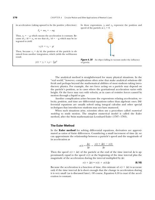
Figure 6.18 An object falling in vacuum under the influence
of gravity.
In the Euler method for solving differential equations, derivatives are approximated
as ratios of finite differences. Considering a small increment of time �t, we
can approximate the relationship between a particle’s speed and the magnitude of
its acceleration as
a(t) �
�v
�t
� v(t ��t) � v(t)
�t
Then the speed v(t ��t) of the particle at the end of the time interval �t is approximately
equal to the speed v(t) at the beginning of the time interval plus the
magnitude of the acceleration during the interval multiplied by �t:
v(t ��t) � v(t) � a(t)�t
(6.10)
Because the acceleration is a function of time, this estimate of v(t ��t) is accurate
only if the time interval �t is short enough that the change in acceleration during
it is very small (as is discussed later). Of course, Equation 6.10 is exact if the acceleration
is constant.
mg