Circular Motion and Other Applications of Newton's Laws

6.5 Numerical Modeling in Particle Dynamics 171
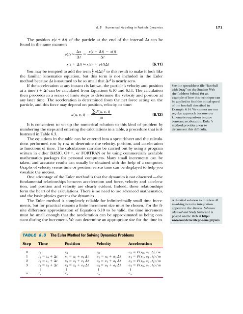
The position x(t ��t) of the particle at the end of the interval �t can be
found in the same manner:
(6.11)
You may be tempted to add the term to this result to make it look like
the familiar kinematics equation, but this term is not included in the Euler
method because �t is assumed to be so small that �t 2 is nearly zero.
If the acceleration at any instant t is known, the particle’s velocity and position
at a time t ��t can be calculated from Equations 6.10 and 6.11. The calculation
then proceeds in a series of finite steps to determine the velocity and position at
any later time. The acceleration is determined from the net force acting on the
particle, and this force may depend on position, velocity, or time:
a(x, v, t) � (6.12)
It is convenient to set up the numerical solution to this kind of problem by
numbering the steps and entering the calculations in a table, a procedure that is illustrated
in Table 6.3.
The equations in the table can be entered into a spreadsheet and the calculations
performed row by row to determine the velocity, position, and acceleration
as functions of time. The calculations can also be carried out by using a program
written in either BASIC, C��, or FORTRAN or by using commercially available
mathematics packages for personal computers. Many small increments can be
taken, and accurate results can usually be obtained with the help of a computer.
Graphs of velocity versus time or position versus time can be displayed to help you
visualize the motion.
One advantage of the Euler method is that the dynamics is not obscured—the
fundamental relationships between acceleration and force, velocity and acceleration,
and position and velocity are clearly evident. Indeed, these relationships
form the heart of the calculations. There is no need to use advanced mathematics,
and the basic physics governs the dynamics.
The Euler method is completely reliable for infinitesimally small time increments,
but for practical reasons a finite increment size must be chosen. For the finite
difference approximation of Equation 6.10 to be valid, the time increment
must be small enough that the acceleration can be approximated as being constant
during the increment. We can determine an appropriate size for the time in-
�F(x,
1
2
v, t)
m
a(�t)2
�x x(t ��t) � x(t)
v(t) � �
�t �t
x(t ��t) � x(t) � v(t)�t
TABLE 6.3 The Euler Method for Solving Dynamics Problems
Step Time Position Velocity Acceleration
0 t 0 x0 v0 a 0 � F(x 0, v0, t 0)/m
1 t 1 � t 0 ��t x1�x0�v0�t v1�v0�a0�t a1�F(x1, v1, t 1)/m
2 t 2 � t 1 ��t x2�x1�v1�t v2�v1�a1�t a2�F(x2, v2, t 2)/m
3 t 3 � t 2 ��t x3�x2�v2�t v3�v2�a2�t a3�F(x3, v3, t 3)/m
n
�
tn �
xn �
vn �
an See the spreadsheet file “Baseball
with Drag” on the Student Web
site (address below) for an
example of how this technique can
be applied to find the initial speed
of the baseball described in
Example 6.14. We cannot use our
regular approach because our
kinematics equations assume
constant acceleration. Euler’s
method provides a way to
circumvent this difficulty.
A detailed solution to Problem 41
involving iterative integration
appears in the Student Solutions
Manual and Study Guide and is
posted on the Web at http:/
www.saunderscollege.com/physics