AP Calculus

Recommendations

Info

Special Focus: The Fundamental Theorem of Calculus 3. (a) Using a graphing calculator, here is the table of values. x 1 2 3 4 5 6 erf(x) 0.84270 0.99532 0.99998 1.00000 1.00000 1.00000 x –1 –2 –3 –4 –5 –6 –0.84270 –0.99532 –0.99998 –1.00000 –1.00000 –1.00000 erf(x) (b) The table in part (a) suggests as x → ∞, erf ( x) → 1, and as x → −∞, erf ( x) → −1. Therefore, technology and the table suggest lim erf ( x) = 1 x→∞ and lim erf ( x) = −1. x→−∞ These limits, if true, indicate the graph of y = erf(x) has two horizontal asymptotes: y = 1 and y = –1. 2 − (c) Using the FTC, erf ′( x) = e x 2 . 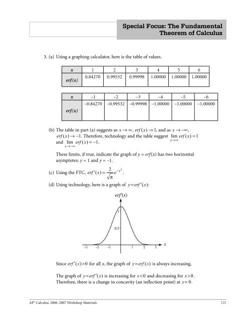π (d) Using technology, here is a graph of y = erf ′( x): Since erf ′( x) > 0 for all x, the graph of y = erf ( x) is always increasing. The graph of y erf x = ′( ) is increasing for x 0 . Therefore, there is a change in concavity (an inflection point) at x = 0. AP® Calculus: 2006–2007 Workshop Materials 121
Special Focus: The Fundamental Theorem of Calculus The graph of y = erf ( x) is concave up on the interval ( −∞, 0 ) and concave down on the interval ( 0, ∞ ). 2 0 2 −t (e) erf ( 0) = ∫ e dt = 0. π 0 Using technology, here is a graph of y = erf ( x). Notice that this graph confirms the results obtained in parts (a) through (d). 4. (a) h(x) is defined as the composition of two functions. Although we do not have a specific rule for the function f, we can still simplify the derivative of h: 2 . h( x) = ( f g)( x) = f ( g( x)) = f ( x ) We use the chain rule to obtain that h′ ( x ) d = = ′ dx f ( x 2 ) f ( x 2 )( 2 x) . (b) Let G( x) = x 2 x −t 10 and F( x) = ∫ ( t − 4) e dt. 0 x Then ( F G)( x) = F( G( x)) = F( x 2 2 − ) = ( t − 4) e t 10 dt = H( x) . ∫ 0 2 2 2 − 10 As in part (a), H′ ( x) = ( 2x) F′ ( x ) = ( 2x)( x − 4) e x 2 2 −x 10 (c) H '( x) = 0⇔( 2x)( x − 4) e = 0 ⇔ 2x = 0 or x 2 − 4 = 0 or e x Thus we conclude that H′ ( x) = 0 ⇔ x = 0 or x = ± 2 (since e x never zero). . − 2 10 = − 2 10 is 0. 122 AP® Calculus: 2006–2007 Workshop Materials
Page 1 and 2:
AP ® Calculus 2006-2007 Profession
Page 3 and 4:
The College Board: Connecting Stude
Page 5 and 6:
Table of Contents Stage Four: Confi
Page 7 and 8:
Special Focus: The Fundamental Theo
Page 9 and 10:
Page 11 and 12:
Page 13 and 14:
Page 15 and 16:
Page 17 and 18:
Page 19 and 20:
Page 21 and 22:
Page 23 and 24:
Page 25 and 26:
Page 27 and 28:
Page 29 and 30:
Page 31 and 32:
Page 33 and 34:
Page 35 and 36:
Page 37 and 38:
Page 39 and 40:
Page 41 and 42:
Page 43 and 44:
Page 45 and 46:
Page 47 and 48:
Page 49 and 50:
Page 51 and 52:
Page 53 and 54:
Page 55 and 56:
Page 57 and 58:
Page 59 and 60:
Page 61 and 62:
Page 63 and 64:
Page 65 and 66:
Page 67 and 68:
Page 69 and 70:
Page 71 and 72:
Page 73 and 74: Special Focus: The Fundamental Theo
Page 123: Special Focus: The Fundamental Theo
Page 131 and 132: Contact Us College Board Regional O
show all

AP Calculus

You also want an ePaper? Increase the reach of your titles

Delete template?

Save as template?