Almost universal parametrizations for cubic surfaces

Computer Aided Geometric Design 20 (2003) 189–207 

www.elsevier.com/locate/cagd 

Almost universal parametrizations for cubic surfaces 

Rainer Müller 

Immenbarg 10, D-22417 Hamburg, Germany 

Received 15 October 2002; received in revised form 23 February 2003; accepted 23 February 2003 

Abstract 

Universal parametrizations have been developed as an useful tool for working with rational surfaces. For 

example, they allow the systematic classification of rational curves with low degree on the surface and can 

be used for interpolation problems. Unfortunately, it is conjectured, that not every rational surface has a 

universal parametrization. To make the advantages usable for more surfaces, we introduce “almost universal 

parametrizations” as a generalization of universal parametrizations. We present them exemplarily for a special 

class of cubic surfaces, which do probably not possess a universal parametrization, and show applications. 

© 2003 Elsevier Science B.V. All rights reserved. 

Keywords: Almost universal parametrization; Cubic surfaces; Parabolic cyclides; Rational curves and patches; Interpolation 

1. Introduction 

Algebraic surfaces are a widespread tool in CAGD. For modelling, it is often necessary to find curves 

and patches in rational parametric form, which are completely contained in a given implicit surface. 

A simple method to find rational curves on a surface is the use of a rational parametrization of the 

surface. Such a parametrization maps every rational curve in the plane to a rational curve on the surface. 

If it is even birational, then every rational curve on the surface is found this way (possibly except some 

exceptional curves). The problem is, that this method in general cannot represent every curve with its 

lowest possible degree, because common factors of the polynomials can arise. They can be cancelled, but 

it is very difficult to predict, for which plane curves such factors arise and what the effective degree of 

the image curve after cancelling is. 

The same method is usable to find patches on the surface, and it has the same disadvantage. As most 

statements for patches are completely similar to those for curves, we will mainly consider curves in the 

following. For shortness, “curve” will always stand for “rational curve”. 

E-mail address: rainermmueller@planet-interkom.de (R. Müller). 

0167-8396/03/$ – see front matter © 2003 Elsevier Science B.V. All rights reserved. 

doi:10.1016/S0167-8396(03)00024-4

190 R. Müller / Computer Aided Geometric Design 20 (2003) 189–207 

In contrast to usual parametrizations, universal parametrizations allow not only to represent every 

curve, but also every possible parametrization of such a curve (possibly except some exceptional curves), 

especially those with optimal (i.e., minimal) degree, so that no cancelling is necessary. 

Such universal parametrizations were first found for the sphere (Dietz et al., 1993), then for all quadrics 

(Dietz, 1995) and Dupin cyclides (Mäurer, 1997a, 1997b). (Krasauskas, 1997) gave the general concept 

and first definition of “universal parametrizations”. (Müller, 2002) gives universal parametrizations for 

different types of cubic surfaces and serves also as an introduction to universal parametrization. 

It is an open question, whether every rational surface has a universal parametrization or not, but it is 

conjectured, that the universally parametrizable surfaces are exactly the toric surfaces (see (Krasauskas, 

2000, 2001) for an introduction to toric surfaces; the conjecture has not been published yet). The cubic 

surfaces were classified completely by Schläfli into several species and are therefore available for a 

systematic treatment. Three of these species are toric, the others are not, and exactly for the toric species 

universal parametrizations were found. 

As universal parametrizations have proven to be useful, but seem not to exist for all rational surfaces, 

it is desirable to have some weaker form of universal parametrization. On the one hand, the requirements 

for such a mapping cannot be as strong as those for universal parametrizations, so that they do exist for 

more surfaces than the universally parametrizable ones, but on the other hand, they may not be too weak, 

because else they would not be very useful. Several ways for such a generalization are possible. 

The aim of this paper is to present one possible generalization, that we call almost universal 

parametrizations. They are a real generalization in the sense, that every universal parametrization is 

an almost universal parametrization. We will deduce them exemplarily for a certain species of non-toric 

cubics, so they do exist for surfaces, which do conjecturally not have a universal parametrization, and for 

these surfaces we will show, that we can use them almost as good for the classification of rational curves 

on the surface and interpolation as universal parametrizations. 

The paper is organized as follows. In the next section we will explain, how common factors in rational 

parametrizations arise, and define universal parametrizations. After this, we present in Section 3 the 

different types of surfaces we will treat in this article. An almost universal parametrization for surfaces 

of the first type will be deduced in Section 4, where we will also give a general definition of such 

parametrizations. Sections 5 and 6 present the classification of curves and interpolation as applications 

for the almost universal parametrization. In Section 7 we present almost universal parametrizations for 

the two other types. 

2. Rational curves and universal parametrizations 

Rational curves and patches are most easily described in homogeneous coordinates of the projective 

space P 3 , which represent an euclidian point p = ( ˆx, ˆy, ˆz) ∈ R 3 by any vector in R 4 spanning the subspace 

R · (1, ˆx, ˆy, ˆz), while the vectors spanning a different one-dimensional subspace represent the points at 

infinity. We write x ∼ x ′ ,whenx and x ′ are homogeneous coordinates of the same point, i.e., iff x = λx ′ 

with a λ ∈ R \{0}. In difference, x = x ′ means equality of the quadruples. 

A rational parametrization X of a curve (or patch) is written in homogeneous coordinates as 

a quadruple X = (w,x,y,z) of polynomials. The cases of curves and patches can be treated 

simultaneously, when we write R[−] for any of the rings R[τ] or R[σ,τ]. R[−] is a factorial ring,

R. Müller / Computer Aided Geometric Design 20 (2003) 189–207 191 

so that every element can be written as a product of irreducible factors, which is unique up to order and 

unit elements. 

When a parametrization X = (w,x,y,z) has a common zero τ0 of all four components, X(τ0) is not 

defined, it is a base point. By (repeated) cancelling of the common factor (τ − τ0), X(τ0) can be defined 

continuously, but while the base point formally interpolates any given point, the continuation does not, 

so base points have to be avoided for interpolation. 

Common factors are the reason, why not every curve on a given surface can be represented with 

optimal degree via a birational parametrization ψ. Birationality means ψ(ψ −1 (X)) = λX with a λ ∈ R. 

When X is a rational curve, then λ will be a polynomial in the curve parameter, which is in general not 

constant, so that deg ψ(ψ −1 (X)) > deg X. For example, the well known stereographic projection onto 

the sphere is a birational parametrization, but no circle on the sphere except those containing the center 

of projection can be parametrized with the optimal degree two via this parametrization. 

A universal parametrization of a surface X treats the possible curves or patches X on X not only as 

sets of quotients, whose components can be scaled with a arbitrary factor, but as quadruples in R[−] 4 . 

Especially the coprime quadruples, i.e., the parametrizations without common factors, which include 

all parametrizations with optimal degree, are images under such a universal parametrization. Abstractly, 

rational curves resp. patches are solutions of the equation f(w,x,y,z) = 0 in the ring R[−],whenf = 0 

describes X in the real space. A universal parametrization is a parametric description of the solutions of 

this diophantine equation. The following is an exact definition. 

Definition 1. A universal parametrization of a rational algebraic surface X ⊂ P3 is a polynomial mapping 

γ : Rk → X with a k ∈ N, so that every mutually prime solution X = (w,x,y,z) of the homogeneous 

equation of the surface in a ring of real polynomials R[τ] or R[σ,τ], i.e., every curve resp. every patch 

on the surface, is the image of a curve resp. a patch in Rk under γ , 

(w,x,y,z)= γ(Y) for a Y ∈ R[τ] k � resp. Y ∈ R[σ,τ] k� , (1) 

if X is not a parametrization of a curve out of a finite set E of exceptional curves on X. 

γ is allowed to be defined only on a dense set D ⊆ Rk and give the null vector for points in Rk \ D. 

When such a universal parametrization is found, it can be used to classify the curves of low degree 

on the surface systematically, to construct rational patches in certain regions of the surface and to solve 

interpolation problems. This is done elaborately for several types of cubic surfaces in (Müller, 2002). The 

rationality and the degree of a curve or patch do not change under projective transformations. Therefore, 

we can describe the rational curves and patches on a surface X, when we have something like a universal 

parametrization for a surface X ′ , which is projectively equivalent to X. Hence, it suffices to consider only 

one surface of each projective equivalence class to apply the results to all surfaces of this class. 

3. Cubics with four nodes and parabolic cyclides 

Cubic surfaces or cubics for short are more flexible than quadrics, but their still low degree makes 

computations easier and allows a complete classification. Furthermore, all cubics except elliptic cones 

are rational. Therefore they have often been treated in classical geometry and CAGD. 

Here we consider one special class of cubics, namely those with four nodes (species 16 in Schäflis 

classification of cubics (Schläfli, 1863)). A node is a singular point, which has a neighbourhood without


any other singular points. A cubic can have at most four nodes, and in complex space all cubics with four 

nodes are equivalent. Nonreal nodes of real surfaces occur in complex conjugated pairs, so that three real 

projective equivalence classes or “types” of real cubics with four nodes exist, whose members have 0, 2 

resp. 4 real nodes. For this article, we choose the following symmetric standard surfaces: 

w � x 2 + y 2� + x � w 2 + z 2� = 0 for type 1: no real nodes, (2) 

w � x 2 + y 2� + x � w 2 − z 2� = 0 for type 2: two real nodes, (3) 

w � x 2 − y 2� + x � w 2 − z 2� = 0 for type 3: four real nodes. (4) 

As these three equations are very similar to each other, the following work would be quite similar for all 

types. 

These surfaces are not toric (the toric surfaces of low degree are completely listed in (Krasauskas, 

2001), also see (Müller, 2002)). Hence, according to Krasauskas’ conjecture they do not possess universal 

parametrizations. We will deduce parametric representations of the solutions of their equations and see, 

why we do not achieve universal parametrizations. But we will find representations, which are almost 

as good and will therefore be almost universal parametrizations. In this paper, we will consider the 

surface (2) of type 1 elaborately, for it we will show applications of the almost universal parametrizations. 

For the other types, we will only present such parametrizations, which can be applied analogously. 

Before this, we want to mention the parabolic cyclides as a metric special case of cubics with four 

nodes. All curvature lines of a cyclide are circles (or lines as degenerate circles with infinite radius). 

General surfaces with this property are called Dupin Cyclides, they are algebraic surfaces of order four. 

They have been treated several times, (Boehm, 1990; Pratt, 1990) deal especially with their applications 

in CAGD. (Mäurer, 1997a) derives a universal parametrization for Dupin cyclides, in addition (Mäurer, 

1997b) also gives an introduction to these surfaces. 

Some special cases of cyclides have lower degree than four: trivial cases are planes, spheres and cones, 

moreover there are cyclides of degree three, namely the so called parabolic cyclides. (Srinivas and Dutta, 

1995) derives a rational parametrization and emphasizes the usefulness of these surfaces for applications 

in geometric design, because the existence of straight lines of curvature provides a smooth transition 

from planar to curved surfaces. 

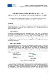
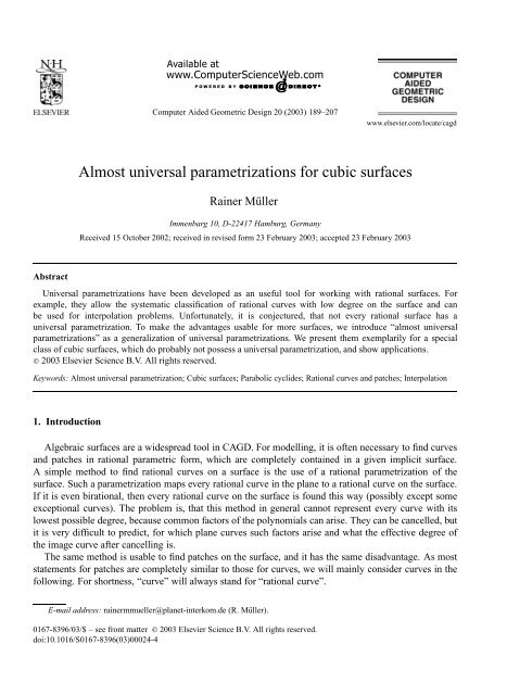
Fig. 1. Parabolic cyclides (left, middle) and standard surface (2) of type 1.


In general, a parabolic cyclide has four nodes, from which either none or exactly two are real, i.e., 

parabolic cyclides belong to the types 1 and 2 of the cubics we treat in this paper. The different types are 

called parabolic ring cyclides and parabolic spindle cyclides. A special case, which we do not consider, 

appears, when two nodes coincide (parabolic horn cylides). 

Fig. 1 shows on the left a parabolic spindle cyclide and in the middle a parabolic ring cyclide. All 

drawn curves are circles or straight lines. 

Parabolic cyclides have already been treated in the context of universal parametrization (Mäurer, 

1997b; Krasauskas and Mäurer, 2000), but until now, no universal parametrization was found. Hence, 

they are a good starting point to look for a generalization of Definition 1 to make the concept of universal 

parametrization usable for further surfaces. 

4. Almost universal parametrization 

We consider the standard surface (2) for surfaces of type 1. It is drawn in Fig. 1 on the right. 

Theorem 2. Let (w,x,y,z)be a coprime solution of (2) in R[−], and let w and x both not be zero. Then 

exist polynomials d,x1,x2,x3,x4,y1,y2,y3,y4,z1,z2 ∈ R[−], so that 

w = � x 2 1 + x2 � 2 

2 dz1 = � x 2 1 + x2 � 1 

2 

x =− � x 2 3 + x2 � 2 

4 dz2 =− � x 2 3 + x2 4 

d (x3h3 − x4h4) 2 , 

� 1 

d (x1h1 − x2h2) 2 , 

y =− � x 2 3 + x2 � 

4 z2(x1h2 + x2h1) =− � x 2 3 + x2 4 

� 1 

d (x1h1 − x2h2)(x1h2 + x2h1), 

z = � x 2 1 + x2 � 

2 z1(x3h4 + x4h3) = � x 2 1 + x2 � 1 

2 

d (x3h3 − x4h4)(x3h4 + x4h3) 

with the abbreviations 

h1 = y1y2 + y3y4, h2 = y1y3 − y2y4, h3 = y1y2 − y3y4, h4 = y1y3 + y2y4, 

where the eleven variables fulfill the constraints 

dz1 = x3h3 − x4h4 = x3y1y2 − x3y3y4 − x4y1y3 − x4y2y4, 

dz2 = x1h1 − x2h2 = x1y1y2 + x1y3y4 − x2y1y3 + x2y2y4. 

Versed, (5) is a solution of (2) for all d,x1,x2,x3,x4,y1,y2,y3,y4,z1,z2 ∈ R[−], which fulfill (6). 

The complete proof is given in Appendix A. Due to the constraints (6), the quotients in (5) exist in 

R[−], and both representations are equal. 

This theorem describes all solutions of the equation in a parametric manner, but these parameters are 

not arbitrary, they must fulfill certain equations. Hence, (5) can be interpreted as a mapping from R 11 

to P 3 , but the image is only contained in the given surface, when the domain is restricted to a set with 

codimension two. But for our purposes, construction of curves and interpolation, we need the variables 

to be free. 

Nevertheless, the theorem helps us finding many of the possible solutions. To do so, we consider the 

meaning of the constraints (6). They say simply, that the variable d is a common divisor of two terms, 

(5) 

(6)


and the variables z1 and z2 are the quotients of these terms divided by this common divisor. As the terms 

are quite complicated, we did not succeed in finding a parametric representation. But in special cases, 

the constraints become trivial, namely when d is an unit in the ring of polynomials, i.e., a constant. Then 

the equations can be solved for z1 resp. z2. In (5) we see, that d is a common divisor of the first two 

components w and x of the solution. Hence, if these components are coprime, then we can solve the 

constraints and get a representation of the solution in the remaining variables, which may be arbitrary 

polynomials. 

This is the content of the following corollary. The constant d can be normed to 1 or −1, it is the sign 

of w and therefore renamed to s. 

Corollary 3. Let (w,x,y,z)be a solution of (2) in R[−],wherewand x are coprime and both not zero. 

Then exist polynomials x1,x2,x3,x4,y1,y2,y3,y4 ∈ R[−] and a homogeneous factor s ∈{1, −1}, so that 

w = s � x 2 1 + x2 � 

2 (x3h3 − x4h4) 2 , 

x =−s � x 2 3 + x2 � 

4 (x1h1 − x2h2) 2 , 

(7) 

y =−s � x 2 3 + x2 � 

4 (x1h1 − x2h2)(x1h2 + x2h1), 

z = s � x 2 1 + x2 � 

2 (x3h3 − x4h4)(x3h4 + x4h3) 


h1 = y1y2 + y3y4, h2 = y1y3 − y2y4, h3 = y1y2 − y3y4, h4 = y1y3 + y2y4. 

Versed, (7) is a solution of (2) for all x1,x2,x3,x4,y1,y2,y3,y4,s ∈ R[−]. 

(7) can be interpreted as a mapping γ from R 8 onto the surface (2). The corollary says, that 

every solution of (2) in real polynomials in one or two variables, i.e., every curve or patch on the 

surface, is the image of a curve or patch under this map, if its first two components are coprime. This 

excludes infinitely many different solutions, but the set of excluded solutions is still “small” compared 

to the set of all solutions. Therefore, such a representation of solutions should still be useful and is 

a possible generalization of the concept of universal parametrizations. If we define almost universal 

parametrizations as follows, γ is such an almost universal parametrization, where the exceptional curves, 

which arise from the requirement w �= 0 �= x in Corollary 3, are the three straight lines g1: w = x = 0, 

g2: w = z = 0andg3: x = y = 0. 

Definition 4. An almost universal parametrization of a rational algebraic surface X ⊂ P3 is a polynomial 

mapping γ : Rk → X with a k ∈ N, so that every mutually prime solution X = (w,x,y,z) of the 

homogeneous equation of the surface in a ring of real polynomials R[τ] or R[σ,τ], i.e., every curve 

resp. every patch on the surface, is the image of a curve resp. a patch in Rk under γ , 

(w,x,y,z)= γ(Y) for a Y ∈ R[τ] k � resp. Y ∈ R[σ,τ] k� , (8) 

if X is not a parametrization of a curve out of a finite set E of exceptional curves on X and if l1(X) and 

l2(X) are coprime, where l1 and l2 are two linear indepent, linear, homogeneous functions in w,x,y,z. 

γ is allowed to be defined only on a dense set D ⊆ Rk and give the null vector for points in Rk \ D. 

The only difference between this definition and Definition 1 of a universal parametrization is, that 

we do not claim to describe all mutually prime solutions X, but only those solutions, where the two


polynomials l1(X) and l2(X) are coprime. This notion is necessary to achieve a projectively invariant 

definition. When a suitable coordinate system is chosen, we can assume l1(X) = w and l2(X) = x,sowe 

consider solutions, where the two first components are coprime, as we have done in Corollary 3. 

If all four components of a solution X have a common factor, then no two linear homogeneous 

functions l1(X) and l2(X) can be coprime. Hence, every universal parametrization is an almost universal 

parametrization, where l1 and l2 can be chosen arbitrarily, and the almost universal parametrizations are 

indeed a generalization of universal parametrizations. 

In the case of curves, the coprimeness of l1(X) and l2(X) can be interpreted geometrically. Two real 

univariate polynomials are coprime, iff they have no common zero in C. Therefore l1(X) and l2(X) are 

coprime, iff for no finite value τ the point X(τ) lies on the straight line l1 = l2 = 0. A curve with only 

one point on this line can be parametrized, so that this point corresponds to τ =∞. Hence, the required 

coprimeness of Definition 4 excludes exactly those curves, who have more than one common point with 

l1 = l2 = 0. 

For a parabolic cyclide, a representation of all solutions with coprime w and x is implicitly given in 

(Krasauskas and Mäurer, 2000). It is given not directly for the surface, but for its canonical isotropic 

hypersurface, which corresponds to it in Laguerre geometry. By intersection of the hypersurface with 

P3 and solving a diophantine equation in this parametrization, one gets a representation, which is 

projectively equivalent to our almost universal parametrization. 

For more convenient work with γ we note the following. We do not need the factor s, because we 

can rescale a solution with −1, when necessary. As (7) is homogeneous in each of the pairs (x1,x2), 

(x3,x4), (y1,y4) and (y2,y3), we can interpret the domain of γ as a direct product of four projective 

lines, whose homogeneous coordinates are these pairs, which we will denote by u, v, s and t, where 

u = (u0,u1) = (x1,x2) etc. Furthermore, the abbreviations hi induce a natural decomposition of γ in two 

mappings, the first of which maps s and t to hi, the second being (7) with the hi as variables. The image 

of the first mapping is the one-sheeted hyperboloid H : h2 1 + h2 2 − h2 3 − h2 4 = 0. We name the first mapping 

ϑH , the second γH . They are given by 

ϑH : � P 1� 2 → H, 

� (s0,s1), (t0,t1) � ↦→ (s0t0 + s1t1,s0t1 − s1t0,s0t0 − s1t1,s0t1 + s1t0), 

γH : P 1 × P 1 × H → X, 

� (u0,u1), (v0,v1), (h1,h2,h3,h4) � ↦→ 

�� 

2 u0 + u2 � 

1 (v0h3 − v1h4) 2 , − � v2 0 + v2 � 

1 (u0h1 − u1h2) 2 , 

− � v2 0 + v2 � 

1 (u0h1 − u1h2)(u0h2 + u1h1), � u2 0 + u2 � 

1 (v0h3 − v1h4)(v0h4 + v1h3) � . 

With this, we have the almost universal parametrization 

γ : � P 1�4 � 3 

→ P , γ(u, v, s, t) = γH u, v,ϑH (s, t) � . 

Throughout the following we use the notation h = ϑH (s, t). Aside from the use in the following 

section, this decomposition also simplifies the computation of preimages under γ . ϑH is birational with 

ϑ −1 

H (h1,h2,h3,h4) = ((h1 + h3,h4 − h2), (h1 + h3,h4 + h2)), and the preimages under γH are given by 

the following theorem, where B: u0h1 − u1h2 = 0 ∧ v0h3 − v1h4 = 0 describes the exceptional set of 

γH . Combined with ϑH , Eqs. (9) are cubic equations in u, v, s, t.


Theorem 5. Let x = (w,x,y,z) be a real point on the surface (2). x is contained in the image of 

γH ,iffxdoes not lie on the line g1: w = x = 0. Then its preimage under γH 

(u, v, h) ∈ (P 

consists of all points 

1 × P1 × H)\ B, which fulfill the equations 

v0h3 − v1h4 = 0, (yh1−xh2)u0 − (yh2 + xh1)u1 = 0, if w = z = 0, 

u0h1 − u1h2 = 0, (zh3−wh4)v0 − (zh4 + wh3)v1 = 0, if x = y = 0, (9) 

(zh3 − wh4)v0 − (zh4 + wh3)v1 = 0, (yh1−xh2)u0 − (yh2 + xh1)u1 = 0 otherwise. 

5. Classification of curves 

We consider rational curves X on the surface (2). Each such curve can be represented by a mutually 

prime quadruple X = (w,x,y,z)∈ R[−] 4 . For the cases deg X � 3, i.e., for lines, conics and cubics, we 

classify all possible curves and give normal forms. 

5.1. Straight lines and conic sections 

Theorem 6. The surface (2) contains exactly five real straight lines: 

g1: w = x = 0, g2: w = z = 0, g3: x = y = 0, 

g4: w + x = y − z = 0, g5: w + x = y + z = 0. 

Proof. g1,g2 and g3 are the exceptional curves of Theorem 2. Let X = (w,x,y,z) be a different line 

on the surface. Then we have the representation (5). As deg X = 1, the variables x1,x2,x3,x4,z1,z2 and 

therefore x/w need to be constant. Hence X is contained in the intersection of the surface with a plane 

x = cw for a c ∈ R.AsX is not the line g1 at infinity, it is contained in the conic y 2 + cz 2 =−c(c + 1)w 2 , 

which decomposes only for c = 0orc =−1. c = 0 gives the doubly counting line g3, c =−1thetwo 

lines g4 and g5. The latter two can be parametrized as X(t) = (1, −1,t,t)= γ(1, 0, 1, 0, 1,t,1, 0) resp. 

X(t) = (1, −1, −t,t) = γ(1, 0, 1, 0, 1, 0, 1,t). ✷ 

The three lines in euclidian space, g3,g4 and g5, are drawn in the left part of Fig. 2 as degeneracies of 

the drawn conics. 

A plane through a straight line on a cubic intersects the surface besides the line in a conic (which may 

degenerate to a pair of lines). Every conic on a cubic surface lies in a plane, which intersects the surface 

in this conic and a straight line. Hence, there is a bijective correspondence between lines and pencils of 

conics on a cubic surface, so that the surface (2) contains exactly five pencils of conics. We enumerate 

them as Ci, i = 1, 2, 3, 4, 5, according to the lines gi. 

The pencil C1 consists of hyperbolas, two of which degenerate to the doubly counting line g3 resp. 

to the line pair (g4,g5). Each hyperbola has two common points with the line g1 and can therefore 

not be parametrized by γ without common factors. Later we will find cubic parametrizations of these 

hyperbolas, that can be described by γ . Fig. 2 shows on the left some hyperbolas of this pencil, the three 

lines g3,g4 and g5 are marked. 

The pencil C2 consists of circles, the three pencils C3, C4 and C5 consist of parabolas. Each curve 

of C4 intersects each curve of C5 in two points, but else, two curves of different of these four pencils


Fig. 2. Left: pencil C 1 of hyperbolas, including the lines g 3,g 4 and g 5. Right: pencils C 4 and C 5 of parabolas. 

intersect in only one point. Therefore, each pair i


Every plane cuts a cubic surface in a plane cubic curve. In general, this intersection curve is an elliptic 

curve. It is a rational curve, iff it contains exactly one singular point P . Either P is a node of the surface, 

or the plane is a tangent plane and touches the surface in P . Hence, the plane cubic curves on a cubic 

surface can be found in a quite easy geometric way. 

But the nonplane cubic curves, the so called twisted cubics, cannot be found so easily. We will show 

in this section, that the almost universal parametrization allows a systematic approach to find and classify 

all cubic curves on the surface, the plane and the twisted ones. In principle, this approach is also possible 

for higher degree curves. As the method is quite technical, we do not present all the details here, they can 

be found in (Müller, 2001). 

Let X = (w,x,y,z) be a cubic curve on the surface (2). None of the four components can be zero, 

so we have the representation (5) with constraints (6) from Theorem 2. For a cubic, the fraction x/w 

may not be constant, so that deg d


is the image of the line s − σbt + a = 0 under the mapping δ25 in the case σ =+1 resp. under δ24 in 

the case σ =−1. We have introduced these mappings in (12) and (11) to describe the pencils C5 and 

C4 of conics, which are images of the lines s = const and excluded here by the requirement b �= 0. Also 

excluded by the normalization are the preimage lines t = const, which are mapped to the circles of pencil 

C2. Hence, analogous to case (i), (17) describes two two-parametric families CU25 (σ =+1) and CU24 

(σ =−1) of cubics, which include the pencils C2 and C5 resp. C2 and C4 as special cases. 

(iii) Let u be constant, v not, u = (1, 0), v = (1,τ). This case is symmetric to (ii), we achieve the 

normal form 

X(τ) = �� (1 − b)τ + a � 2 , −b 2 � 1 + τ 2� , −σb � 1 + τ 2� (τ + a), � (1 − b)τ + a �� τ 2 + aτ + b �� , (18) 

which describes two more two-parametric families CU34 and CU35 of cubics, analogous to (ii) with the 

mappings δ34 and δ35 from (13) and (14) instead of δ24 and δ25. 

(iv) Finally, let u and v both be constant, u = v = (1, 0). Weuseh = ϑH (s, t) for some s, t ∈ R[−] 2 , 

go on as before and achieve the normalized form 

� 

X(τ) = γH 1, 0, 1, 0,ϑH (1,aτ + b, τ, 1) � 

(19) 

with a,b ∈ R, a�= 0. This describes a sixth two-parametric family of cubics, which are the images of 

lines under the mapping δ45 from (15). The curve (19) is cubic only for b �= 0, for b = 0 it describes the 

hyperbolas of pencil C1 in cubic parametrization with the common factor τ , according to a base point at 

τ = 0. 

We summarize the results in the following theorem. 

Theorem 8. The standard surface (2) of cubics with four nonreal nodes contains six two-parametric 

families of (rational) cubic curves. Each family can be represented as family of images of the lines in the 

plane, which are not parallel to an axis, under a rational parametrization of the plane. For five families, 

this mapping is even birational. 

The images of those lines in the plane, which are parallel to an axis, are conics. For the last mapping, 

also the images of all lines through the origin are conics. All quadratic curves on the surface appear as 

degenerate cases of the families of cubic curves. 

The following table lists for every family the rational mapping, the two pencils of conics and the 

number of the equation of the normal form for the curves. The families are named after the included 

conic sections. 

Denotation Mapping s-lines t-lines Normal form 

CU23 δ23 (10) C2 C3 (16) 

CU24 δ24 (11) C2 C4 (17)σ =−1 

CU25 δ25 (12) C2 C5 (17)σ =+1 

CU34 δ34 (13) C3 C4 (18)σ =−1 

CU35 δ35 (14) C3 C5 (18)σ =+1 

CU45 δ45 (15) C4 C5 (19) 

The first five families contain one or two straight lines as border cases: CU23 contains g4 and g5, 

CU24 and CU25 contain g3, CU34 and CU35 contains g2. All other curves of these families except the 

border conics are twisted cubic curves. All curves of CU45 are plane, and with the exception of the three 

mentioned pencils of conics they all are cubic curves. 

(20)


While each two of the pencils C2,C3,C4,C5 determine together a family of cubics, this is not the 

case for the pencil C1. This exceptional property of C1, which is a geometric property, is reflected in the 

almost universal parametrization, as the curves of C1 are the only quadratic curves on the surface, whose 

quadratic parametrizations cannot be represented by the almost universal parametrization. 

5.3. Junction curves 

Theorem 8 can be used to find junction curves of minimal degree between two points. 

Corollary 9. Let p and q be two different points on the surface (2). In general exist exactly seven cubic 

curves on the surface, which contain both points. They are images of lines under the six cubic rational 

maps in Table (20). 

In the exceptional cases, that p and q lie in a plane with a line gi on the surface, but not on the line, 

a conic section of pencil Ci on the surface exists, which contains both points. It is the degenerate case of 

the cubic junction curves of those families of cubics, which contain the pencil Ci. 

The junction curves are found by computing the preimages of p and q under the mappings δ∗ from 

above, joining them by a line and mapping the line onto the surface. Each of the five birational mappings 

gives exactly one junction curve, δ45 gives two. 

For simplicity, we have ignored the special cases, that p or q lies on a exceptional curve of one of the 

mappings δ∗, so that it has none or more than one preimage point. For example, the line g3: x = y = 0is 

not contained in the image δ23(P 2 ). 

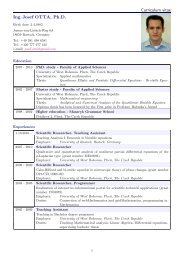
A general example, where seven different cubic junction curves exist, is shown in Fig. 3. Five curves 

between the same end points are drawn together with a part of the surface. The three most straight curves, 

which lie close together, are the two unique curves from the families CU24 and CU34 and one of the two 

CU45 curves. The CU23 curve is the little more arcuate curve, the CU25 curve winds around the other 

side of the surface and is therefore mainly hooded in the figure. The CU35 and the other CU45 curve are 

not drawn, because they contain the points on different branches and are therefore unusable as junction 

Fig. 3. Cubic junction curves on the surface (2).


curves. (As the decomposition into branches is a euclidian property, these curves can be used as junction 

curves on some different surfaces, which are projectively equivalent to (2).) 

5.4. Filling patches 

Often, a patch on a surface shall be constructed as the “filling patch” of a given chain of three or four 

curves on the surface, i.e., it shall be a triangular resp. tensor product patch, whose border lines are the 

given curves. When a birational parametrization ψ of the surface is given, it is possible to fill a chain by 

mapping the border curves into the plane by ψ −1 , filling this plane chain with a planar patch and mapping 

this patch back onto the surface with ψ. But in general, the degree of this patch is higher than the degree 

of its border curves. So, the question is, whether a chain of curves of (low) degree can be filled by a patch 

of the same degree, e.g., whether a given chain of cubic curves can be filled by a cubic patch (this means 

cubic triangular resp. bicubic tensor product patch). In fact, this question was proposed in (Krasauskas, 

1997) as the main problem to be solved with universal parametrizations. 

We can answer this question with our almost universal parametrization, as we could do, if we had a 

universal parametrization. The answer for surface (2) is negative: it is not always possible to fill a chain 

of cubic curves on the surface with a cubic patch. 

For example, take a chain C of one CU24 curve and two or three CU34 curve and assume, it could 

be filled by a cubic triangular resp. bicubic tensor product patch X. As said above, X is representable 

via the almost universal parametrization: X = γH (u, v, h). Hence C can be parametrized as an image 

of a closed chain �C in P1 × P1 × H , namely the boundary of the preimage of X. ButtheCU24 curve 

can be parametrized only with u of degree 1, while the other segments of C can be parametrized only 

with constant u. Therefore, if we walk around C, thevalueofuchanges along the first segment, but not 

along the other segments, so that it has a different value, when we return to the starting point. This is a 

contradiction to the closedness of �C. Hence, no such filling patch exists. 

If all curves of a given chain belong to the same family CU∗, then it is possible to fill the chain, because 

the curves are images of lines in the plane, which form a closed triangle or quadrangle. Filling this plane 

polygon gives the preimage of a cubic filling patch. 

This also means, that we can construct cubic patches with given corner points by first constructing 

junction curves of a certain family as border curves and then filling the chain, or, what is essentially the 

same, by mapping the corner points in the plane by a mapping δ−1 ∗ , constructing a planar patch between 

these preimage points and mapping this back onto the surface (in the case of δ45 different preimage points 

can be chosen, so the δ45 patch is not unique, while the other δ∗ patches are). 

As an example, Fig. 4 shows six bicubic tensor product patches with the same corner points, each 

constructed with a different parametrization δ∗. 

6. Interpolation 

An important task when working with an algebraic surface X is to interpolate a given set of points 

by a curve or a patch on the surface. We consider mainly the curve case, because the case of patches is 

similar but a little more technical. Hence, given are points pi and different parameter values τi, andwe 

look for a curve X on X, which interpolates the points at the given values, i.e., X(τi) ∼ pi for all i.


Fig. 4. Bicubic tensor product patches with given corner points. 

When we have a universal parametrization γ of X, we can work as follows. We check, whether the 

points are contained in one of the (finitely many) exceptional curves of γ . In such a case, this curve is 

an interpolating curve. Else, every possible interpolating curve is the image of a curve under γ ,sowe 

interpolate the preimages γ −1 (pi) with a curve Y in the preimage space R k and set X = γ(Y). Dueto


the properties of a universal parametrization we know, that no cancelling of common factors in X will be 

necessary, and that it is good to choose the degree of Y as low as possible. 

When we do not have a universal parametrization, but only an almost universal parametrization, like 

the one we derived for surface (2) and therewith for all cubics with four complex nodes, we can work 

with this parametrization as we would do with a universal parametrization. Of course, we can not get 

every possible interpolating curve with this parametrization in a representation of optimal degree, but at 

least most of them. 

In (Müller, 2002) was shown, that it is difficult to use a universal parametrization directly for 

interpolation purposes, because the interpolation conditions for the preimage curve Y are nonlinear 

equations in the unknown coefficients, and this system can hardly be solved. Hence, for interpolation 

some birational mappings were used, which were derived from the universal parametrization during 

classifying the curves of low degree, as we have done here in the previous chapter, when deriving the 

mappings δ∗. We will see, that the same problems arise, when we try to interpolate with the almost 

universal parametrization. Therefore, it is better to use the mappings δ∗ for interpolation. As they were 

derived from the almost universal parametrizations just the way they would have been derived from a 

universal parametrization, we see again, that this new kind of parametrization is similarly useful as a 

universal parametrization. 

An example for interpolation on the surface (2) shows the arising problems: We want to interpolate 

the three points (10, −1, 3, 0), (10, −5, 5, 0) and (10, −9, 3, 0) at parameter values 0, 1/2 and1.The 

points were chosen on the circle x2 + y2 + wx = 0, z = 0, which is contained in the surface. Hence, the 

quadratic parametrization 

X(τ) = � 8τ 2 − 8τ + 10, −(2τ + 1) 2 , −(2τ + 1)(2τ − 3), 0 � 

= γ(2τ + 1, 2τ − 3, 0, 1, 1, 1, 1/2, 1/2) (21) 

of this circle is a solution of the interpolation problem. With the general algorithm sketched above, i.e., 

if we do not “see” the circle, we let Y be a general linear curve to get the interpolation curve X = γ(Y). 

Then (9) gives a system of six cubic equations in 16 unknowns. This system has at least one solution, 

namely the one from (21), but the computer algebra system Maple does not find any solution. Reducing 

the number of unknown coefficients of Y by choosing s and t as constants can, in theory, not increase the 

number of solutions, but due to the simplification, Maple does find 16 solutions. Eight of these solutions 

do not lead to interpolation curves, because they describe preimage curves outside the domain of γ , i.e., 

these curves are mapped to the constant zero vector. The other eight solutions are constant multiples of 

the solution (21). 

The example shows, that solutions of the system, even if they exist, are already for small problems 

(only three points) hard to find. As γ is homogeneous in u, v, s and t, every common zero of only one 

of these pairs of variables gives a base point, where the interpolation equations are trivially fulfilled, but 

where the curve does in general not interpolate the point. Hence it is difficult to avoid such base points, 

especially when trying numerical methods to find approximations for solutions. 

The use of a birational map δ∗ can not prevent base points, as it leads to a usual rational interpolation 

problem, but they do not occur so often. As an example, Fig. 5 shows an interpolating curve of degree 12 

through 7 points, which was computed with δ25. 

As algebraic curves of high degree tend to have bows or loops, it could be useful to choose spline 

curves as preimage curves.


Fig. 5. Interpolating curve on the surface (2). 

7. Almost universal parametrizations for the other types 

The derivation of almost universal parametrization for the standard surfaces (3) and (4) of the two 

other types of cubics with four nodes is quite similar to the proceeding for the first type in Section 4, 

so we present only the results. The two theorems below are analogous to Corollary 3, they are actually 

corollaries to theorems like Theorem 2 (these theorems and proofs can be found detailed in (Müller, 

2001)). 

As in the previous section for surface (2), interpolation problems can be solved in theory directly 

via the almost universal parametrizations, in practice it would surely be better to derive birational 

parametrizations from the classification of curves. 

Theorem 10 (Surfaces with two real nodes). Let (w,x,y,z) be a solution of (3) in R[−], wherew 

and x are coprime and both not zero. Then exist polynomials x1,x2,x3,x4,y1,y2,y3, y4∈ R[−] and a 

homogeneous factor s ∈{1, −1}, so that 

w = s � x2 1 + x2 � 

2 (x3h3 − x4h4) 2 , 

x =−4sx3x4(x1h1 − x2h2) 2 , 

y =−4sx3x4(x1h1 − x2h2)(x1h2 + x2h1), 

z = s � x2 1 + x2 � 

2 (x3h3 − x4h4)(x3h3 + x4h4) 


h1 = y1y3 − y2y4, h2 = y1y4 + y2y3, h3 = y 2 1 + y2 2 , h4 =− � y 2 3 + y2 � 

4 . 

Versed, (22) is a solution of (3) for all x1,x2,x3,x4,y1,y2,y3,y4,s∈ R[−]. 

Fig. 6 shows the standard surfaces of types 2 and 3 and a different surface of type 3, where all four 

nodes can be seen. This figure shows the symmetry of the surface with respect to its four nodes, which 

form the corners of a regular tetrahedron. 

(22)


Fig. 6. Standard surfaces of type 2 (left) and 3 (middle) and surface with four visible nodes. 

Corollary 11 (Surfaces with four real nodes). Let (w,x,y,z)be a solution of (4) in R[−], wherewand x are coprime and both not zero. Then exist polynomials x1,x2,x3,x4,y1,y2,y3, y4∈ R[−], so that 

w = x1x2(x3h3 − x4h4) 2 , 

x = x3x4(x1h1 − x2h2) 2 , 

y = x3x4(x1h1 − x2h2)(x1h1 + x2h2), 

z = x1x2(x3h3 − x4h4)(x3h3 + x4h4) 


h1 = y1y2, h2 =−y3y4, h3 = y1y3, h4 = y2y4. 

Versed, (23) is a solution of (4) for all x1,x2,x3,x4,y1,y2,y3,y4 ∈ R[−]. 

A remarkable fact is, that the cubic with four nodes, which seems to have no universal parametrization, 

is dual to a surface, which has a universal parametrization, namely Steiner’s Roman surface, a surface of 

degree four with three double lines and a triple point (Müller, 2002). 

8. Conclusion 

We have seen, that almost universal parametrizations can be nearly as useful as universal parametrizations. 

Hence, it is reasonable to look for such parametrizations for other surfaces, which may not have a 

universal parametrization. 

For the derivation of almost universal parametrizations we tried to find a parametric representation 

of all solutions of the surface’s equation as a diophantine equation in the ring of polynomials. This is 

the same proceeding as the derivation of universal parametrizations. Therefore, the further search for 

almost universal parametrizations could either lead to a counterexample against Krasauskas’ conjecture, 

that only the toric surfaces possess a universal parametrization, or to a proof of it. Especially, it would be 

interesting to find connections between the property “toric” and the structure of the diophantine equation. 

The question of necessary or sufficient conditions for existence also arises for almost universal 

parametrizations. As said above, Definition 4 is just one possible generalization to the definition 

of universal parametrizations. Possibly a different definition would be better in the sense, that a 

(23)


parametrization of this kind would exist for all rational surfaces, but still guarantees the usefulness of 

such a parametrization. 

Appendix A. Proof of Theorem 2 

Let (w,x,y,z)∈ R[−] 4 be a solution of (2) with gcd(w,x,y,z)= 1. We set d = gcd(w, x), w = dw ′ , 

x = dx ′ .Asd �= 0, (2) is equivalent to 

w ′� (dx ′ ) 2 + y 2� + x ′� (dw ′ ) 2 + z 2� = 0. (A.1) 

As w ′ and x ′ are coprime, w ′ |z2 follows, thus z2 = w ′ p0 with a p0 ∈ R[−]. Every irreducible divider 

of z divides either w ′ or p0 quadratic or both factors once. With p2 = gcd(w ′ ,p0) we get the 

representation w ′ = p2 1p2, p0 = p2p2 3 ,z= p1p2p3 with p1,p2,p3 ∈ R[−], whereatp1and p3 are 

coprime. Analogously x ′ |y2 holds and therefore y = p4p5p6, x ′ = p2 4p5 with p4,p5,p6 ∈ R[−] and 

coprime p4,p6. Putting in (A.1) and cancelling of p2 1p2p2 4p5 = w ′ x ′ �= 0 yields 

� 2 

p5 ˜p 4 + p 2� � 2 

6 + p2 ˜p 1 + p 2� 3 = 0 (A.2) 

with ˜p1 = dp1, ˜p4 = dp4. Asw ′ and x ′ are coprime, p2 and p5 are also coprime, so that p2|( ˜p 2 4 + p2 6 ) 

follows. We use the factorization in C[−]: p2|( ˜p4 + ip6)( ˜p4 − ip6). Suppose, ˜p4 and p6 have a nontrivial 

common prime divider q. Asp4 and p6 are coprime, q isacommondividerofdand p6, hence because 

of d|w,x and p6|y a common divider of w,x and y. Furthermore, due to (A.2) and q|d| ˜p1, q is also 

adividerofp2p2 3 , and from the irreducibility of q follows q|p2p3|z. But this is a contradiction to 

the coprimeness of the solution. Hence, ˜p4 and p6 are coprime. Then ˜p4 + ip6 and ˜p4 − ip6 are also 

coprime, especially they do not possess a real irreducible factor. Each nontrivial irreducible factor of p2 

in R[−] must therefore split in C[−] into two complex conjugated factors, one of which dividing ˜p4 +ip6 

and the other dividing ˜p4 − ip6: p2 = c1(p7 + ip8)(p7 − ip8), ˜p4 + ip6 = (p7 + ip8)(p9 + ip10), with 

p7,p8,p9,p10 ∈ R[−] and c1 ∈{−1, 1}, as every positive real number can be written as product of two 

complex conjugated numbers. 

Completely analogous, from (A.2) follow p5|( ˜p 2 1 + p2 3 ), the coprimesness of ˜p1 and p3 and therewith 

the existence of p11,p12,p13,p14 ∈ R[−] and c2 ∈{1, −1}, sothatp5 = c2(p11 + ip12)(p11 − ip12) and 

˜p1 + ip3 = (p11 + ip12)(p13 + ip14). Putting in (A.2) and cancelling of c2p2p5 yields 

p 2 9 + p2 10 

+ c1 

c2 

� 2 

p13 + p 2 � 

14 = 0. 

For real polynomials, c2 = c1 is only possible for the trivial solution p9 = p10 = p13 = p14 = 0, which 

leads to w = x = y = z = 0. Hence, c2 =−c1 and the equation can be transformed to 

(p9 + p13)(p9 − p13) = (p14 + p10)(p14 − p10). 

Geometrically, this is a one-sheeted hyperboloid, the general solution is given by p9 + p13 = 2y1y2, 

p9 − p13 = 2y3y4, p14 + p10 = 2y1y3, p14 − p10 = 2y2y4 with y1,y2,y3,y4 ∈ R[−]. We introduce the 

factors 2 to achieve a convenient presentation: p9 = y1y2 + y3y4, p13 = y1y2 − y3y4, p14 = y1y3 + 

y2y4, p10 = y1y3 − y2y4. Therewith we have shown: 

dp1 =˜p1 = p11(y1y2 − y3y4) − p12(y1y3 + y2y4), 

dp4 =˜p4 = p7(y1y2 + y3y4) − p8(y1y3 − y2y4),


� 2 

p2 = c1 p7 + p 2� 8 , 

� 2 

p5 =−c1 p11 + p 2 � 

12 , 

p3 = p11(y1y3 + y2y4) + p12(y1y2 − y3y4), 

p6 = p7(y1y3 − y2y4) + p8(y1y2 + y3y4). 

The last four equations simply express the variables p2,p3,p5,p6 by other ones, but the first and 

the second cannot simply be solved for one single variable, as they mean, that the polynomial d is a 

common divider of the two right hand sides. They are constraints to the polynomials. By renaming of 

variables, p7 = x1,p8 = x2,p11 = x3,p12 = x4,p1 = z1,p4 = z2, and replacing the polynomials z1,z2 

and d by c1z1,c1z2 and c1d, i.e., multiplying with −1, if necessary, the factor c1 cancels, and we get the 

representation (5) for the solution and (6) for the constraints. The polynomials p9,p10,p13,p14, which are 

not arbitrary but fulfill the equation of a hyperboloid, which is universally parametrized by y1,y2,y3,y4, 

appear as abbreviations h1,h2,h3,h4 in (5). 

The converse, that (5) is a solution of (2) for all d,x1,...,z2, which fulfill (6), is true, because we only 

used equivalence transformations in the derivation, or simply checked by putting in. 

References 

Boehm, W., 1990. On cyclides in geometric modeling. Computer Aided Geometric Design 7, 243–255. 

Dietz, R., 1995. Rationale Bézier-Kurven und Bézier-Flächenstücke auf Quadriken. Diss. TH Darmstadt, Shaker, Aachen. 

Dietz, R., Hoschek, J., Jüttler, B., 1993. An algebraic approach to curves and surfaces on the sphere and on other quadrics. 

Computer Aided Geometric Design 10, 211–229. 

Krasauskas, R., 1997. Universal parameterizations of some rational surfaces. In: Le Méhauté, A., Rabut, C., Schumaker, L.L. 

(Eds.), Curves and Surfaces with Applications in CAGD. Vanderbilt University Press, Nashville, TN. 

Krasauskas, R., 2000. Toric surface patches I, Preprint 2000-21, Faculty of Mathematics and Informatics, Vilnius University. 

Krasauskas, R., 2001. Shape of toric surfaces, Preprint 2001-06, Faculty of Mathematics and Informatics, Vilnius University, 

http://www.maf.vu.lt/katedros/cs2/cagl/tor_surf.htm, to appear in the SCCG Conference Proceedings. 

Krasauskas, R., Mäurer, C., 2000. Studying cyclides with Laguerre geometry. Computer Aided Geometric Design 17, 101–126. 

Mäurer, C., 1997a. Generalized parameter representations of tori, Dupin cyclides and supercyclides. In: Le Méhauté, A., 

Rabut, C., Schumaker, L.L. (Eds.), Curves and Surfaces with Applications in CAGD. Vanderbilt University Press, Nashville, 

TN. 

Mäurer, C., 1997b. Rationale Bézier-Kurven und Bézier-Flächenstücke auf Dupinschen Zykliden. Diss. TH Darmstadt, Shaker, 

Aachen. 

Müller, R., 2001. Universelle Parametrisierung und Interpolation auf kubischen Flächen. Diss. TU Darmstadt, Shaker, Aachen. 

Müller, R., 2002. Universal parametrization and interpolation on cubic surfaces. Computer Aided Geometric Design 19, 479– 

502. 

Pratt, M.J., 1990. Cyclides in computer aided geometric design. Computer Aided Geometric Design 7, 221–242. 

Schläfli, L., 1863. On the Distribution of Surfaces of the Third Order into Species, in reference to the absence or presence of 

Singular Points, and the reality of their Lines. Philos. Trans. Roy. Soc. London 153, 193–241. Nachdruck in Gesammelte 

Mathematische Abhandlungen, Band II. Birkhäuser, Basel, 1953, 304–362. 

Srinivas, Y.L., Dutta, D., 1995. Rational parametric representation of parabolic cyclides: Formulation and applications. 

Computer Aided Geometric Design 12, 551–566.

Almost universal parametrizations for cubic surfaces

You also want an ePaper? Increase the reach of your titles

Delete template?

Save as template?