

Mathematical Modeling of Influenza Viruses

You also want an ePaper? Increase the reach of your titles
YUMPU automatically turns print PDFs into web optimized ePapers that Google loves.
<strong>Mathematical</strong> <strong>Modeling</strong> <strong>of</strong> <strong>Influenza</strong> <strong>Viruses</strong><br />
Project Number: MA-RYL-1314<br />
A Major Qualifying Project<br />
submitted to the Faculty<br />
<strong>of</strong> the<br />
WORCESTER POLYTECHNIC INSTITUTE<br />
in partial fulfillment <strong>of</strong> the requirements for the<br />
Degree <strong>of</strong> Bachelor <strong>of</strong> Science<br />
by<br />
Linan Zhang<br />
Tianyu Li<br />
Zhaokun Xue<br />
March 14, 2014<br />
Approved<br />
Pr<strong>of</strong>essor Roger Y. Lui<br />
Major Advisor
Abstract<br />
This Major Qualifying Project can be divided into three parts. We first start<br />
with the simplest SIR model to describe the transmission <strong>of</strong> communicable disease<br />
through individuals. We analyze the SIR model and the SEIR model with<br />
periodic transmission rates. With a constant transmission rate in the SIR or<br />
SEIR model, the occurrence <strong>of</strong> an epidemic outbreak depends on the Basic Reproduction<br />
Number <strong>of</strong> the model. But with a periodic transmission rate, small<br />
amplitude periodic solutions exhibiting a sequence <strong>of</strong> period-doubling bifurcations<br />
may appear. Then we focus on the two-strain SIR model with constant transmission<br />
rate. The two-strain model displays three basic relationships between the<br />
two viruses: coexistence, replacement, and periodic alternation between coexistence<br />
and replacement. These relationships are determined by the existence and<br />
stability <strong>of</strong> each equilibrium point. If there is no stable equilibrium point, the<br />
two-strain model has periodic solutions. We also study the two-strain SIR model<br />
with periodic transmission rate. The last part <strong>of</strong> this project conerns patterns<br />
observed from data downloaded from the World Health Organization (WHO) on<br />
the infective individuals <strong>of</strong> H1N1(77), H1N1(09), and H3N2(68) viruses.<br />
1
Acknowledgments<br />
We would like to thank Pr<strong>of</strong>essor Roger Lui <strong>of</strong> the <strong>Mathematical</strong> Sciences Department<br />
for his continuous advice and assistance throughout this project. We would<br />
also like to thank Pr<strong>of</strong>essor Daihai He <strong>of</strong> the Applied Mathematics Department,<br />
Hong Kong Polytechnic University, who assisted us in building the two-strain SIR<br />
model and downloading data from WHO.<br />
2
Contents<br />
1 Introduction 7<br />
1.1 Biology Background . . . . . . . . . . . . . . . . . . . . . . . . . . . . . . . . 7<br />
1.1.1 Classification <strong>of</strong> <strong>Influenza</strong> <strong>Viruses</strong> . . . . . . . . . . . . . . . . . . . . . 7<br />
1.1.2 <strong>Influenza</strong> Pandemic . . . . . . . . . . . . . . . . . . . . . . . . . . . . . 8<br />
1.1.3 Antigenic Drift . . . . . . . . . . . . . . . . . . . . . . . . . . . . . . . 10<br />
1.1.4 Antigenic Shift . . . . . . . . . . . . . . . . . . . . . . . . . . . . . . . 11<br />
1.2 The One-Strain SIR Model . . . . . . . . . . . . . . . . . . . . . . . . . . . . . 11<br />
2 The One-Strain <strong>Influenza</strong> Models with Periodic Transmission Rate 14<br />
2.1 Analysis <strong>of</strong> the SIR Model . . . . . . . . . . . . . . . . . . . . . . . . . . . . . 14<br />
2.2 Analysis <strong>of</strong> the SEIR Model . . . . . . . . . . . . . . . . . . . . . . . . . . . . 19<br />
2.3 Effective Infectee Number <strong>of</strong> the SEIR Model . . . . . . . . . . . . . . . . . . 24<br />
3 The Two-Strain <strong>Influenza</strong> Model 27<br />
3.1 Introduction . . . . . . . . . . . . . . . . . . . . . . . . . . . . . . . . . . . . . 27<br />
3.2 Analyses <strong>of</strong> the Equilibrium Points . . . . . . . . . . . . . . . . . . . . . . . . 28<br />
3.2.1 Analysis <strong>of</strong> E 1 . . . . . . . . . . . . . . . . . . . . . . . . . . . . . . . . 29<br />
3.2.2 Analysis <strong>of</strong> E 2 . . . . . . . . . . . . . . . . . . . . . . . . . . . . . . . . 29<br />
3.2.3 Analysis <strong>of</strong> E 3 . . . . . . . . . . . . . . . . . . . . . . . . . . . . . . . . 31<br />
3.2.4 Analysis <strong>of</strong> E 4 . . . . . . . . . . . . . . . . . . . . . . . . . . . . . . . . 33<br />
4 Stability <strong>of</strong> Interior Equilibrium Points 35<br />
4.1 Analyses <strong>of</strong> the Model ( when ) F 0 < 1 . . . . . . . . . . . . . . . . . . . . . . . . 35<br />
4.1.1 0 < β < γ 1 + δ 1<br />
δ 2<br />
. . . . . . . . . . . . . . . . . . . . . . . . . . . . . 36<br />
4.1.2 γ<br />
(<br />
1 + δ 1<br />
4.1.3 2γ < β < γ<br />
4.1.4 γ<br />
)<br />
δ 2<br />
< β < 2γ . . . . . . . . . . . . . . . . . . . . . . . . . . . . 36<br />
( )<br />
1 + δ 2<br />
δ 1<br />
. . . . . . . . . . . . . . . . . . . . . . . . . . . . 38<br />
(<br />
1 + δ 2<br />
δ 1<br />
)<br />
< β < (2 + δ 2 − δ 1 )γ + (δ 2 − δ 1 ) . . . . . . . . . . . . . . . . 39<br />
4.2 Analyses <strong>of</strong> the Model when F 0 > 1 . . . . . . . . . . . . . . . . . . . . . . . . 40<br />
4.2.1 Stability <strong>of</strong> E 4 . . . . . . . . . . . . . . . . . . . . . . . . . . . . . . . . 40<br />
4.2.2 Stability <strong>of</strong> E 1 . . . . . . . . . . . . . . . . . . . . . . . . . . . . . . . . 42<br />
4.2.3 Existence and Stability <strong>of</strong> E 2 and E 3 . . . . . . . . . . . . . . . . . . . 42<br />
3
5 Effects <strong>of</strong> Transmission Rate in the Two-strain Model 47<br />
5.1 Two-strain SIR Model with Constant Transmission Rate . . . . . . . . . . . . 47<br />
5.1.1 Coexistence . . . . . . . . . . . . . . . . . . . . . . . . . . . . . . . . . 48<br />
5.1.2 Replacement . . . . . . . . . . . . . . . . . . . . . . . . . . . . . . . . . 48<br />
5.1.3 Periodic and Alternating Coexistence and Replacement . . . . . . . . . 48<br />
5.2 Two-strain SIR Model with Periodic Transmission Rate . . . . . . . . . . . . . 50<br />
5.2.1 Coexistence . . . . . . . . . . . . . . . . . . . . . . . . . . . . . . . . . 50<br />
5.2.2 Replacement . . . . . . . . . . . . . . . . . . . . . . . . . . . . . . . . . 51<br />
5.2.3 Periodic and Alternating Coexistence and Replacement . . . . . . . . . 51<br />
6 Analysis <strong>of</strong> the WHO Data 57<br />
6.1 Downloading Data from FluNet . . . . . . . . . . . . . . . . . . . . . . . . . . 57<br />
6.2 Interpolation <strong>of</strong> the Data . . . . . . . . . . . . . . . . . . . . . . . . . . . . . . 58<br />
6.3 Interpretation <strong>of</strong> the Data . . . . . . . . . . . . . . . . . . . . . . . . . . . . . 58<br />
6.3.1 Replacement <strong>of</strong> H1N1(77) by H1N1(09) . . . . . . . . . . . . . . . . . . 58<br />
6.3.2 Coexistence <strong>of</strong> H1N1 and H3N2(68) . . . . . . . . . . . . . . . . . . . . 60<br />
6.3.3 Skips <strong>of</strong> H1N1(09) and H3N2(68) . . . . . . . . . . . . . . . . . . . . . 61<br />
7 Conclusion 64<br />
A List <strong>of</strong> Symbols 69<br />
B Matlab Scripts 70<br />
B.1 SIRperiodic.m . . . . . . . . . . . . . . . . . . . . . . . . . . . . . . . . . . . . 70<br />
B.2 SEIRstable.m . . . . . . . . . . . . . . . . . . . . . . . . . . . . . . . . . . . . 71<br />
B.3 SIRSIR.m . . . . . . . . . . . . . . . . . . . . . . . . . . . . . . . . . . . . . . 72<br />
B.4 SIRSIRplot.m . . . . . . . . . . . . . . . . . . . . . . . . . . . . . . . . . . . . 78<br />
B.5 simulateE4.m . . . . . . . . . . . . . . . . . . . . . . . . . . . . . . . . . . . . 82<br />
B.6 E4root.m . . . . . . . . . . . . . . . . . . . . . . . . . . . . . . . . . . . . . . 84<br />
4
List <strong>of</strong> Figures<br />
1.1 Trajectories <strong>of</strong> the SIR Model with γ = 1 and β = 2 . . . . . . . . . . . . . . . 13<br />
2.1 Trajectories <strong>of</strong> the SIR Model with γ = 1 and β = 3 and µ = 1 . . . . . . . . . 16<br />
2.2 − log(I) vs. t and − log(I) vs. − log(S) <strong>of</strong> the SIR Model with κ = 0.07 . . . . 17<br />
2.3 − log(I) vs. t and − log(I) vs. − log(S) <strong>of</strong> the SIR Model with κ = 0.08 . . . . 17<br />
2.4 − log(I) vs. t and − log(I) vs. − log(S) <strong>of</strong> the SIR Model with κ = 0.0875 . . 18<br />
2.5 − log(I) vs. t and − log(I) vs. − log(S) <strong>of</strong> the SIR Model with κ = 0.09 . . . . 18<br />
2.6 − log(I) vs. t and − log(I) vs. − log(S) <strong>of</strong> the SEIR Model with κ = 0.03 . . . 21<br />
2.7 − log(I) vs. t and − log(I) vs. − log(S) <strong>of</strong> the SEIR Model with κ = 0.05 . . . 22<br />
2.8 − log(I) vs. t and − log(I) vs. − log(S) <strong>of</strong> the SEIR Model with κ = 0.05 . . . 22<br />
2.9 − log(I) vs. t and − log(I) vs. − log(S) <strong>of</strong> the SEIR Model with κ = 0.08 . . . 23<br />
2.10 − log(I) vs. t and − log(I) vs. − log(S) with κ = 0.1 . . . . . . . . . . . . . . 23<br />
2.11 − log(I) vs. t and − log(I) vs. − log(S) <strong>of</strong> the SEIR Model with κ = 0.15 . . . 24<br />
2.12 − log(I) vs. t and − log(I) vs. − log(S) <strong>of</strong> the SEIR Model with κ = 0.25 . . . 24<br />
2.13 − log(I) vs. t and − log(I) vs. − log(S) <strong>of</strong> the SEIR Model with κ = 0.26 . . . 25<br />
2.14 − log(I) vs. t and − log(I) vs. − log(S) <strong>of</strong> the SEIR Model with κ = 0.27 . . . 25<br />
4.1 E 1 is stable; E 2 , E 3 , and E 4 do not exist . . . . . . . . . . . . . . . . . . . . . 37<br />
4.2 E 1 is unstable; E 3 is stable; E 2 and E 4 do not exist . . . . . . . . . . . . . . . 38<br />
4.3 E 1 and E 2 are unstable; E 3 is stable; E 4 does not exist . . . . . . . . . . . . . 40<br />
4.4 E 1 and E 3 are unstable; E 2 does not exist; E 4 is stable . . . . . . . . . . . . . 43<br />
4.5 E 1 , E 3 , and E 4 are unstable; E 2 does not exist . . . . . . . . . . . . . . . . . . 44<br />
4.6 E 1 , E 2 , and E 3 are unstable; E 4 is stable . . . . . . . . . . . . . . . . . . . . . 45<br />
4.7 E 1 , E 2 , E 3 , and E 4 are all unstable . . . . . . . . . . . . . . . . . . . . . . . . 46<br />
5.1 Coexistence between virus 1 and virus 2 . . . . . . . . . . . . . . . . . . . . . 48<br />
5.2 Replacement <strong>of</strong> virus 2 by virus 1 . . . . . . . . . . . . . . . . . . . . . . . . . 49<br />
5.3 Periodic alternation between coexistence and replacement . . . . . . . . . . . . 49<br />
5.4 Coexistence between virus 1 and virus 2 with κ = 0.1 and κ = 0.4 . . . . . . . 50<br />
5.5 Replacement <strong>of</strong> virus 2 by virus 1 with κ = 0.1 and κ = 0.4 . . . . . . . . . . . 52<br />
5.6 Periodic and alternating coexistence and replacement with κ = 0.1 . . . . . . . 53<br />
5.7 Periodic and alternating coexistence and replacement with κ = 0.2 . . . . . . . 54<br />
5.8 Periodic and alternating coexistence and replacement with κ = 0.3 . . . . . . . 55<br />
5.9 Periodic and alternating coexistence and replacement with κ = 0.4 . . . . . . . 56<br />
6.1 Replacement <strong>of</strong> H1N1(77) by H1N1(09) in some European and Asian regions . 59<br />
6.2 Coexistence <strong>of</strong> H1N1(77) and H3N2(68) in the American regions . . . . . . . . 61<br />
5
6.3 Coexistence <strong>of</strong> H1N1(09) and H3N2(68) in the American regions (Due to the<br />
magnitude, the peaks <strong>of</strong> H3N2(68) are hard to see) . . . . . . . . . . . . . . . 62<br />
6.4 Skips <strong>of</strong> H1N1(09) and H3N2(68) in the European regions . . . . . . . . . . . 63<br />
6
Chapter 1<br />
Introduction<br />
<strong>Influenza</strong>, commonly known as ”flu”, is an infectious disease <strong>of</strong> birds and mammals caused<br />
by RNA viruses <strong>of</strong> the family Orthomyxoviridae, the influenza viruses (Urban, 2009). It can<br />
cause mild to severe illness. Serious outcomes <strong>of</strong> flu infection can result in hospitalization or<br />
death. Some people, such as the old, the young, and those with certain health conditions, are<br />
at high risk for serious flu complications (Unknown, 2013a).<br />
Epidemiologists use systems <strong>of</strong> differential equations to model the number <strong>of</strong> people infected<br />
with a virus in a closed population over time. The simplest system is the Kermack-<br />
McKendrick model.<br />
1.1 Biology Background<br />
1.1.1 Classification <strong>of</strong> <strong>Influenza</strong> <strong>Viruses</strong><br />
In virus classification, influenza viruses are RNA viruses that make up three <strong>of</strong> the five genera<br />
<strong>of</strong> the family Orthomyxoviridae: <strong>Influenza</strong>virus A, <strong>Influenza</strong>virus B, and <strong>Influenza</strong>virus<br />
C. The type A <strong>Influenza</strong> viruses are the most virulent human pathogens among the three<br />
influenza types and cause the severest disease. The influenza A virus can be subdivided into<br />
11 different serotypes based on the antibody response to hemagglutinin and neuraminidase<br />
which form the basis <strong>of</strong> the H and N. These serotypes are: H1N1, H2N2, H3N2, H5N1, H7N7,<br />
H1N2, H9N2, H7N2, H7N3, H10N7, H7N9, (Hay et al., 2001)(Hilleman, 2002). Wild aquatic<br />
birds are the natural hosts for a large variety <strong>of</strong> influenza A (Mettenleiter and Sobrino, 2008).<br />
As for influenza B virus, it almost exclusively infects humans and is less common than influenza<br />
A (Hay et al., 2001). The only other animals known to be susceptible to influenza B<br />
infection are the seal (Osterhaus et al., 2000) and the ferret (Jakeman et al., 1994). <strong>Influenza</strong><br />
C virus, which infects humans, dogs, and pigs, sometimes causing both severe illness and local<br />
epidemics, is less common than the other types (Matsuzaki et al., 2002)(Taubenberger and<br />
Morens, 2008).<br />
7
1.1.2 <strong>Influenza</strong> Pandemic<br />
A pandemic is a worldwide disease outbreak. It is determined by how the disease spreads not<br />
how many deaths it causes. When an influenza virus especially influenza A virus emerges, an<br />
influenza pandemic can occur (Unknown, 2013e).<br />
<strong>Influenza</strong> pandemics usually occur when a new strain <strong>of</strong> the influenza virus is transmitted<br />
to humans from another animal species. Pigs, chickens, and ducks are thought to be<br />
important in the emergence <strong>of</strong> new human strains. <strong>Influenza</strong> A viruses can occasionally be<br />
transmitted from wild birds to other species, which causes outbreaks in domestic poultry and<br />
gives rise to human influenza pandemics (Kawaoka, 2006)(Mettenleiter and Sobrino, 2008).<br />
WHO has produced a six-phase classification that describes the process by which a novel<br />
influenza virus moves from the first few infections in humans through to a pandemic. These<br />
six phases also reflect WHO’s risk assessment <strong>of</strong> the global situation regarding each influenza<br />
virus with pandemic potential that infects humans (Unknown, 2013b). These six phases are<br />
followed by post-peak period and post-pandemic period (Unknown, 2009b).<br />
Phase 1: No viruses circulating among animals have been reported to cause infections in<br />
humans.<br />
Phase 2: An animal influenza virus circulating among domesticated or wild animals is<br />
known to have caused infection in humans, and is therefore considered a potential pandemic<br />
threat.<br />
Phase 3: An animal or human-animal influenza reassortant virus has caused sporadic cases<br />
or small clusters <strong>of</strong> disease in people, but has not resulted in human-to-human transmission<br />
sufficient to sustain community-level outbreaks.<br />
Phase 4: This phase is characterized by verified human-to-human transmission <strong>of</strong> an animal<br />
or human-animal influenza reassortant virus able to cause community-level outbreaks.<br />
The ability to cause sustained disease outbreaks in a community marks a significant upwards<br />
shift in the risk for a pandemic.<br />
Phase 5: Characterized by human-to-human spread <strong>of</strong> the virus into at least two countries<br />
in one WHO region.<br />
Phase 6: Characterized by community level outbreaks in at least one other country in a<br />
different WHO region in addition to the criteria defined in Phase 5.<br />
Post-Peak Period: During the post-peak period, pandemic disease levels in most countries<br />
with adequate surveillance will have dropped below peak observed levels.<br />
Post-Pandemic Period: In the post-pandemic period, influenza disease activity will have<br />
returned to levels normally seen for seasonal influenza.<br />
8
Until now, four main influenza pandemics have occurred throughout history:<br />
1918 - 1920<br />
1918 flu pandemic (January 1918 - December 1920) was an unusually deadly influenza pandemic.<br />
And it was the first <strong>of</strong> the two pandemics involving H1N1 influenza virus (the second<br />
being the 2009 flu pandemic) (Taubenberger and Morens, 2006). At that time, to maintain,<br />
morale, wartime censors minimized early reports <strong>of</strong> illness and mortality in Germany,<br />
Britain, France, and the United States; but papers were free to report the epidemic’s effects<br />
in neutral Spain (such as the grave illness <strong>of</strong> King Alfonso XIII), creating a false impression<br />
<strong>of</strong> Spain as especially hard hit, thus the pandemic’s nickname Spanish flu (Galvin). On<br />
the U.S. Department <strong>of</strong> Health & Human Services website’s 1918 flu pandemic report, it<br />
announces that approximately 20% to 40% <strong>of</strong> the worldwide population became ill, around<br />
50 million people died, and nearly 675,000 people died in the United States (Unknown, 2013f).<br />
1957 - 1958<br />
1957 flu pandemic is also called the Asian flu, which is the H2N2 subtype <strong>of</strong> influenza A. Asian<br />
flu pandemic outbreak originated in China in early 1956, and lasted until 1958 (Greene, 2006).<br />
Estimates <strong>of</strong> worldwide deaths vary widely depending on source, ranging from 1 million to 4<br />
million, with WHO settling on ”about two million.” Death toll in the US was approximately<br />
69,800 (Greene and Moline, 2006). The elderly people had the highest rates <strong>of</strong> death. The<br />
Asian flu strain later evolved via antigenic shift into H3N2, which caused a milder pandemic<br />
from 1968 to 1969 (Hong, 2006).<br />
1968 - 1969<br />
The 1968-70 pandemic or Hong Kong flu was also relatively mild compared to the Spanish<br />
flu (Unknown, 2013d). The Hong Kong flu was a category 2 flu pandemic. It was caused<br />
by an H3N2 strain <strong>of</strong> influenza A virus which descended from H2N2.The Hong Kong flu affected<br />
mainly the elderly and killed approximately one million people in the world (Mandel,<br />
2009)(Paul, 2008)(Unknown, 2009a). In the US, there were about 33,800 deaths (Unknown,<br />
2013c).<br />
2009 - 2010<br />
The most recent one is 2009 flu pandemic or swine flu which is the second pandemic involving<br />
H1N1 influenza virus (the first one is the 1918 flu pandemic). On June 11, 2009, Dr.<br />
Margaret Chan, the director <strong>of</strong> WHO, announced that the world now at the start <strong>of</strong> 2009<br />
influenza pandemic. By that time, nearly 30,000 confirmed cases have been reported in 74<br />
countries (Chan, 2009). According to the data on the U.S. Department <strong>of</strong> Health & Human<br />
Services website, by November 2009, 48 states in the United States had reported cases <strong>of</strong><br />
H1N1, mostly in young people. The Centers <strong>of</strong> Disease Control and Prevention (CDC) announced<br />
that approximately 43 million to 89 million people had H1N1 between April 2009<br />
and April 2012 and estimated between 8,870 and 18,300 H1N1 related deaths. On August<br />
10, 2010 WHO declared an end to the global H1N1 flu pandemic (Chan, 2009).<br />
<strong>Influenza</strong> pandemics have caused tremendous impacts on society and economy. The 1918<br />
influenza pandemic claimed 40 million deaths worldwide over 18 months; 675,000 <strong>of</strong> those<br />
9
deaths occurred in the United States. The 1918 influenza also estimated <strong>of</strong> its overall economic<br />
impact range from a 4.25 to a 5.5 percent annual decline in GDP in the US. In addition,<br />
the deaths <strong>of</strong> the 1918 <strong>Influenza</strong> were aged 18 to 40. Such a sudden and irreversible decline<br />
in the labor force would likely produce negative economic consequences in the following years<br />
(Ott, 2008).<br />
Not only the 1918 influenza pandemic led to such huge social and economic impacts to<br />
the United States and the world, but every severe pandemic in the history did lead similarly<br />
disasters on both society and economy to the whole world. Therefore, it is really valuable<br />
for us to work on our project, ”<strong>Mathematical</strong> <strong>Modeling</strong> <strong>of</strong> <strong>Influenza</strong> <strong>Viruses</strong>”. Studying on<br />
this project could help us get better understanding <strong>of</strong> behaviors among two or more influenza<br />
viruses. In the future, our analysis might help us predict possible outcomes and trends <strong>of</strong><br />
influenza viruses outbreaks in advance. This could help us prepare the prevention work early<br />
and reduce the loss as much as possible.<br />
1.1.3 Antigenic Drift<br />
Two processes drive the antigens to change: antigenic drift and antigenic shift. These are<br />
small changes in the virus that happen continually over time, and antigenic drift is more<br />
common than the other. (Earn et al., 2002).<br />
Antigenic drift is the mechanism for variation in viruses that involves the accumulation <strong>of</strong><br />
mutations within the genes that code for antibody-binding sites. This results in a new strain<br />
<strong>of</strong> virus particles which cannot be inhibited as effectively by the antibodies that were originally<br />
targeted against previous strains, making it easier for the virus to spread throughout<br />
a partially immune population (Earn et al., 2002). This process works as follows: a person<br />
infected with a particular flu virus strain develops antibody against that virus. As newer virus<br />
strains appear, the antibodies against the older strains no longer recognize the newer virus,<br />
and reinfection can occur. This is one <strong>of</strong> the main reasons why people can get the flu more<br />
than one time (Unknown, 2011a). Antigenic drift occurs in both influenza A and influenza<br />
B viruses (Earn et al., 2002). The process <strong>of</strong> antigenic drift is best characterized in influenza<br />
type A viruses, and the emergence <strong>of</strong> a new strain <strong>of</strong> influenza A due to antigenic drift can<br />
cause an influenza epidemic or pandemic (Rogers, 2007).<br />
The rate <strong>of</strong> antigenic drift is dependent on two characteristics: the duration <strong>of</strong> the epidemic<br />
and the strength <strong>of</strong> host immunity. A longer epidemic allows for selection pressure<br />
to continue over an extended period <strong>of</strong> time and stronger host immune responses increase<br />
selection pressure for development <strong>of</strong> novel antigens (Earn et al., 2002).<br />
Antigenic drift is also known to occur in HIV (human immunodeficiency virus), which<br />
causes AIDS, and in certain rhinoviruses, which cause common colds in humans. It also has<br />
been suspected to occur in some cancer-causing viruses in humans. Antigenic drift <strong>of</strong> such<br />
viruses is believed to enable the viruses to escape destruction by immune cells, thereby promoting<br />
virus survival and facilitating cancer development (Rogers, 2007).<br />
10
1.1.4 Antigenic Shift<br />
Of greater public health concern is the process <strong>of</strong> antigenic shift also called reassortment.<br />
Antigenic shift is the process by which two or more different strains <strong>of</strong> a virus, or strains <strong>of</strong><br />
two or more different viruses, combine to form a new subtype having a mixture <strong>of</strong> the surface<br />
antigens <strong>of</strong> the two or more original strains. The term is <strong>of</strong>ten applied specifically to influenza<br />
(Narayan and Griffin, 1977). Unlike Antigenic drift which can occur in all kinds <strong>of</strong> influenza,<br />
antigenic shift only occurs in influenza virus A because it can infect not only humans, but<br />
also other mammals and birds (Treanor, 2004) (Zambon, 1999).<br />
Antigenic shift results in a new influenza A subtype or a virus with a hemagglutinin or<br />
a hemagglutinin and neuraminidase combination that has emerged from an animal population<br />
that is so different from the same subtype in humans that most people do not have<br />
immunity to the new virus. Such a shift occurred in the spring <strong>of</strong> 2009, when a new H1N1<br />
virus with a new combination <strong>of</strong> genes emerged to infect people and quickly spread, causing<br />
a pandemic.(Unknown, 2011b)<br />
1.2 The One-Strain SIR Model<br />
The SIR model is an epidemiological model that computes the theoretical number <strong>of</strong> people<br />
infected with a contagious illness in a closed population over time. One <strong>of</strong> the basic one<br />
strain SIR models is Kermack-McKendrick Model. The Kermack-McKendrick Model is used<br />
to explain the rapid rise and fall in the number <strong>of</strong> infective patients observed in epidemics.<br />
It assumes that the population size is fixed (i.e., no births, no deaths due to disease nor by<br />
natural causes), incubation period <strong>of</strong> the infectious agent is instantaneous, and duration <strong>of</strong><br />
infectivity is the same as the length <strong>of</strong> the disease. It also assumes a completely homogeneous<br />
population with no age, spatial, or social structure.<br />
The model consists <strong>of</strong> a system <strong>of</strong> three coupled nonlinear ordinary differential equations:<br />
Ṡ = −βSI<br />
I ˙ = βSI − γI<br />
Ṙ = γI<br />
(1.1a)<br />
(1.1b)<br />
(1.1c)<br />
where S, I and R are the number <strong>of</strong> susceptible, infectious and recovered/immunized individuals<br />
respectively. β is the transmission rate, γ is the recovery rate, and ˙ denotes the derivative<br />
with respective to time t. Let N denote the population size. Clearly,<br />
and<br />
N = S + I + R,<br />
Ṅ = Ṡ + I ˙ + Ṙ = 0.<br />
11
Applying phase-plane analysis to the first two equations, set<br />
and<br />
Ṡ = −βSI = 0,<br />
I ˙ = (βS − γ)I = 0.<br />
(1.2a)<br />
(1.2b)<br />
Therefore, the S-nullclines are<br />
S = 0,<br />
I = 0;<br />
(1.3a)<br />
(1.3b)<br />
and the I-nullclines are<br />
S = γ β ,<br />
I = 0.<br />
(1.4a)<br />
(1.4b)<br />
These three nullclines form a triangle with vertices (0, 0), (N, 0) and (0, N) on the SI-plane.<br />
This triangle is an invariant region <strong>of</strong> steady states. A trajectory always starts from the line<br />
S + I = N, since R(0) = 0. A point is an equilibrium point if and only if Ṡ = I ˙ = Ṙ = 0.<br />
Thus, any trajectory will converge to a point (S, 0) where 0 ≤ S ≤ N.<br />
If S(0) = S 0 < γ , both S(t) and I(t) decreases and converges to a point on the S-axis.<br />
β<br />
There is no outbreak. If S 0 > γ ( ) γ<br />
β , I(t) first increases in the region β , 1 and then decreases<br />
to 0. In this case, an outbreak occurs. See Figure 1.1.<br />
Starting from (S 1 (0), I 1 (0)), both S(t) and I(t) decreases to an equilibrium point on the<br />
S-axis. There is no outbreak. In the contrast, starting from (S 2 (0), I 2 (0)), I(t) first increases,<br />
hitting its maximum where S(t) = γ , and then decreases to 0. Thus, an outbreak occurs.<br />
β<br />
In conclusion, there is a threshold value γ . Define the basic reproduction number (epi-<br />
β<br />
demiological threshold) <strong>of</strong> this model:<br />
R 0 = Nβ<br />
γ<br />
≈ S 0β<br />
γ . (1.5)<br />
Then<br />
S 0 > γ β ⇐⇒ R 0 > 1, (1.6)<br />
and S 0 < γ β ⇐⇒ R 0 < 1. (1.7)<br />
When R 0 < 1, each person who contracts to the disease will infect less than one person before<br />
dying or recovering. When R 0 > 1, the opposite occurs and there will be a outbreak <strong>of</strong><br />
disease.<br />
12
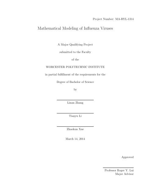
I<br />
S ’ = − beta S I<br />
I ’ = beta S I − gamma I<br />
beta = 2<br />
gamma = 1<br />
1<br />
0.8<br />
0.6<br />
0.4<br />
0.2<br />
0<br />
0 0.2 0.4 0.6 0.8 1<br />
S<br />
Figure 1.1: Trajectories <strong>of</strong> the SIR Model with γ = 1 and β = 2<br />
(S 1 (0), I 1 (0)) = (0.2, 0.8). (S 2 (0), I 2 (0)) = (0.8, 0.2).<br />
Magenta curve: S-nullcline; orange curves: I-nullclines.<br />
Blue curves: trajectories; black curve: invariant line.<br />
13
Chapter 2<br />
The One-Strain <strong>Influenza</strong> Models with<br />
Periodic Transmission Rate<br />
2.1 Analysis <strong>of</strong> the SIR Model<br />
In Chapter 1, we introduced the SIR model (1.1) in which birth rate and death rate are not<br />
taken into account, and the transmission rate β is considered as a constant. Now we assume<br />
(1) that new susceptible are introduced at a constant birth rate µ, (2) that the infectious and<br />
recovered classes experience the same constant birth rate µ, and (3) that all the three classes<br />
experience the same constant death rate, equal to the birth rate µ. The third assumption<br />
ensures that the population size is fixed. For simplicity, set N = 1, which can be achieved by<br />
non-dimensionalization. The new SIR model is:<br />
Ṡ = µ − µS − βSI<br />
I ˙ = βSI − (µ + γ)I<br />
Ṙ = γI − µR<br />
(2.1a)<br />
(2.1b)<br />
(2.1c)<br />
Applying phase-plane analysis to the first two equations, set<br />
and<br />
Ṡ = µ − µS − βSI = 0,<br />
I ˙ = (βS − µ − γ)I = 0.<br />
(2.2a)<br />
(2.2b)<br />
Therefore, the S-nullcline is<br />
and the I-nullclines are<br />
I = µ β<br />
( 1<br />
S − 1 )<br />
, (2.3)<br />
S = µ + γ<br />
β , (2.4a)<br />
I = 0.<br />
(2.4b)<br />
These three nullclines form a triangle with vertices (0, 0), (1, 0) and (0, 1) on the SI-plane.<br />
This triangle is an invariant region <strong>of</strong> steady states. A trajectory always starts from the line<br />
14
S + I = N = 1, since R(0) = 0. The point P 1 = (S1, ∗ I1) ∗ = (1, 0) is always an equilibrium<br />
point, which is a solution <strong>of</strong><br />
S-nullcline: I = µ ( ) 1<br />
β S − 1 , (2.5a)<br />
I-nullcline: I = 0. (2.5b)<br />
The other equilibrium point P 2 = (S2, ∗ I2) ∗ is the solution <strong>of</strong><br />
S-nullcline: I = µ ( ) 1<br />
β S − 1 , (2.6a)<br />
I-nullcline: S = µ + γ<br />
β . (2.6b)<br />
Substitute S ∗ 2 = µ + γ<br />
β<br />
Therefore, the equilibrium point<br />
into (2.2a) and solve for I ∗ 2.<br />
0 = µ − µS2 ∗ − βS2I ∗ 2<br />
∗<br />
0 = µ − µ µ + γ<br />
β<br />
(µ + γ)I ∗ 2 = µ − µ µ + γ<br />
β<br />
I ∗ 2 = µ<br />
µ + γ − µ β<br />
P 2 =<br />
− β µ + γ<br />
β I∗ 2<br />
( µ + γ<br />
β , µ<br />
µ + γ − µ )<br />
β<br />
(2.7)<br />
exists if β > µ + γ. Moreover, using Maple, it is not hard to see that the Jacobian <strong>of</strong> System<br />
(2.1) evaluated at P 2 has no positive eigenvalues. Thus, if P 2 exists, it must be stable.<br />
If S(0) = S 0 < µ + γ , then S(t) increases and I(t) decreases, converging to the equilibrium<br />
point. There is no outbreak. If S 0 > µ + γ , I(t) first increases, and then decreases to<br />
β<br />
β<br />
I2. ∗ In this case, an outbreak occurs. See Figure 2.1.<br />
Starting from (S 1 (0), I 1 (0)), S(t) increases and I(t) decreases to the equilibrium point.<br />
There is no outbreak. In the contrast, starting from (S 2 (0), I 2 (0)), I(t) first increases, hitting<br />
its maximum where S(t) = µ + γ<br />
β<br />
, and then decreases to I∗ 2. Thus, an outbreak occurs.<br />
In conclusion, there is a threshold value µ + γ . Define the basic reproduction number<br />
β<br />
(epidemiological threshold) <strong>of</strong> this model:<br />
R 0 =<br />
β<br />
µ + γ S 0. (2.8)<br />
15
I<br />
S ’ = mu − mu S − beta S I<br />
I ’ = beta S I − (mu + gamma) I<br />
mu = 1<br />
beta = 3<br />
gamma = 1<br />
1<br />
0.8<br />
0.6<br />
0.4<br />
0.2<br />
0<br />
0 0.2 0.4 0.6 0.8 1<br />
S<br />
Figure 2.1: Trajectories <strong>of</strong> the SIR Model with γ = 1 and β = 3 and µ = 1<br />
(S 1 (0), I 1 (0)) = (0.1, 0.9). (S 2 (0), I 2 (0)) = (0.9, 0.1).<br />
Magenta curve: S-nullcline; orange curves: I-nullclines.<br />
Blue curves: trajectories; black curve: invariant line.<br />
Trajectory on the left, starting from (0.1,0.9), shows no outbreak.<br />
Trajectory on the right, starting from (0.9,0.1), shows outbreak.<br />
Then<br />
and<br />
S 0 > µ + γ<br />
β<br />
S 0 < µ + γ<br />
β<br />
⇐⇒ R 0 > 1, (2.9)<br />
⇐⇒ R 0 < 1. (2.10)<br />
When R 0 < 1, each person who contracts to the disease will infect less than one person before<br />
dying or recovering. When R 0 > 1, there will be a outbreak <strong>of</strong> disease.<br />
Now assume that the contact rate β is seasonally varying in time (with period 1 year),<br />
and use a simple sinusoidal form to model it:<br />
where κ is called the degree <strong>of</strong> seasonality and 0 ≤ κ ≤ 1.<br />
β(t) = β 0 (1 + κ cos(2πt)), (2.11)<br />
16
Let S 0 = 0.7, I 0 = 0.3. Fix µ = 0.02, γ = 100, and β = 1800. The following series<br />
<strong>of</strong> figures (Figure 2.2 - 2.5) displays the negation <strong>of</strong> logarithm <strong>of</strong> infective, − log(I), as a<br />
function <strong>of</strong> time and as a function <strong>of</strong> − log(S) for periodic solutions <strong>of</strong> System (2.1). The<br />
corresponding Matlab code can be found in Appendix B.1.<br />
For κ very small, a stable periodical orbit having period 1 emerges from the endemic<br />
equilibrium point P 2 . See Figure 2.2 with κ = 0.07.<br />
13<br />
−log(I) vs. t<br />
13<br />
−log(I) vs. −log(S)<br />
12<br />
12<br />
11<br />
11<br />
−log(I)<br />
10<br />
−log(I)<br />
10<br />
9<br />
9<br />
8<br />
8<br />
7<br />
70 75 80 85 90 95 100<br />
t<br />
7<br />
2.8 2.85 2.9 2.95 3 3.05<br />
−log(S)<br />
Figure 2.2: − log(I) vs. t and − log(I) vs. − log(S) <strong>of</strong> the SIR Model with κ = 0.07<br />
Stable periodical solutions. There is no bifurcation.<br />
As κ increases, past a critical value, the period 1 orbit becomes unstable and a stable<br />
biennial orbit appears. See Figure 2.3 with κ = 0.08 and Figure 2.4 with κ = 0.0875.<br />
15<br />
−log(I) vs. t<br />
15<br />
−log(I) vs. −log(S)<br />
14<br />
14<br />
13<br />
13<br />
12<br />
12<br />
−log(I)<br />
11<br />
−log(I)<br />
11<br />
10<br />
10<br />
9<br />
9<br />
8<br />
8<br />
7<br />
70 75 80 85 90 95 100<br />
t<br />
7<br />
2.75 2.8 2.85 2.9 2.95 3 3.05<br />
−log(S)<br />
Figure 2.3: − log(I) vs. t and − log(I) vs. − log(S) <strong>of</strong> the SIR Model with κ = 0.08<br />
Unstable periodical solutions. Period doubling bifurcation occurs.<br />
17
An important feature <strong>of</strong> the biennial outbreak, or bifurcation, is that alternating years <strong>of</strong><br />
high and low incidence, or effective infectee number, begin to appear, represented as inner<br />
and outer cycles respectively in Figure 2.3. Further information on effective infectee number<br />
and its derivation can be found in Section 2.3.<br />
16<br />
−log(I) vs. t<br />
16<br />
−log(I) vs. −log(S)<br />
15<br />
15<br />
14<br />
14<br />
13<br />
13<br />
−log(I)<br />
12<br />
11<br />
−log(I)<br />
12<br />
11<br />
10<br />
10<br />
9<br />
9<br />
8<br />
8<br />
7<br />
70 75 80 85 90 95 100<br />
t<br />
7<br />
2.75 2.8 2.85 2.9 2.95 3 3.05 3.1 3.15<br />
−log(S)<br />
Figure 2.4: − log(I) vs. t and − log(I) vs. − log(S) <strong>of</strong> the SIR Model with κ = 0.0875<br />
Unstable periodical solutions. Period doubling bifurcation occurs.<br />
Further increments in κ yield chaotic period doubling bifurcation. In (Keeling et al., 2001),<br />
it is explained that nonlinear effects <strong>of</strong> the system play a stronger role than periodic behavior<br />
<strong>of</strong> seasonality. See Figure 2.5 with κ = 0.09.<br />
18<br />
−log(I) vs. t<br />
18<br />
−log(I) vs. −log(S)<br />
16<br />
16<br />
14<br />
14<br />
−log(I)<br />
12<br />
−log(I)<br />
12<br />
10<br />
10<br />
8<br />
8<br />
6<br />
70 75 80 85 90 95 100<br />
t<br />
6<br />
2.7 2.75 2.8 2.85 2.9 2.95 3 3.05 3.1<br />
−log(S)<br />
Figure 2.5: − log(I) vs. t and − log(I) vs. − log(S) <strong>of</strong> the SIR Model with κ = 0.09<br />
Unstable periodical solutions. Bifurcation becomes chaotic.<br />
18
In conclusion, for κ very small, a stable periodical orbit having period 1 emerges from<br />
the nontrivial equilibrium point P 2 . As κ increases, past a critical value, the period 1 orbit<br />
becomes unstable and a stable biennial orbit appears, where occurs the period doubling bifurcation.<br />
Further increments in κ yield chaotic period doubling bifurcation.<br />
2.2 Analysis <strong>of</strong> the SEIR Model<br />
Now consider the population with constant size consisting <strong>of</strong> the fourth class <strong>of</strong> individuals:<br />
the exposed, denoted as E. Then S + E + I + R = 1. Assume that exposed individuals<br />
become infective at a rate α, which leads the SIR model (2.1) to:<br />
Ṡ = µ − µS − βSI<br />
Ė = βSI − (µ + α)E<br />
I ˙ = αE − (µ + γ)I<br />
Ṙ = γI − µR<br />
(2.12a)<br />
(2.12b)<br />
(2.12c)<br />
(2.12d)<br />
Applying phase-plane analysis to the first three equations, set<br />
and<br />
Ṡ = µ − µS − βSI = 0,<br />
Ė = βSI − (µ + α)E = 0,<br />
I ˙ = αE − (µ + γ)I = 0.<br />
(2.13a)<br />
(2.13b)<br />
(2.13c)<br />
Therefore, the S-nullcline is<br />
the E-nullcilne is<br />
I = µ β<br />
E =<br />
( 1<br />
S − 1 )<br />
, (2.14)<br />
β SI, (2.15)<br />
µ + α<br />
and the I-nullcilne is<br />
E = µ + γ I, (2.16)<br />
α<br />
These three nullclines form a tetrahedron with vertices (0, 0, 0), (1, 0, 0), (0, 1, 0) and (0, 0, 1)<br />
on the SEI-plane. This tetrahedron is an invariant region <strong>of</strong> steady states. A trajectory<br />
always starts from the plane S + E + I = N = 1, since R(0) = 0. The point Q 1 =<br />
(S ∗ 1, E ∗ 1, I ∗ 1) = (1, 0, 0) is always an equilibrium point, which clearly satisfies Equation (2.13).<br />
19
The other equilibrium point Q 2 = (S ∗ 2, E ∗ 2, I ∗ 2) can be derived as the following:<br />
β<br />
µ + α S∗ 2I ∗ 2 = µ + γ<br />
α I∗ 2<br />
S2 ∗ (µ + γ)(µ + α)<br />
=<br />
αβ<br />
I2 ∗ = µ ( ) 1 µα<br />
− 1 =<br />
β S2<br />
∗ (µ + γ)(µ + α) − µ β<br />
E2 ∗ = µ + γ<br />
α I∗ 2 = µ µ(µ + γ)<br />
−<br />
µ + α αβ<br />
Therefore, the equilibrium point<br />
( (µ + γ)(µ + α)<br />
Q 2 = (S2, ∗ E2, ∗ I2) ∗ =<br />
,<br />
αβ<br />
µ<br />
µ + α<br />
µ(µ + γ)<br />
− ,<br />
αβ<br />
µα<br />
(µ + γ)(µ + α) − µ )<br />
β<br />
(2.17)<br />
exists if β ><br />
(µ + γ)(µ + α)<br />
.<br />
α<br />
The Jacobian <strong>of</strong> System (2.12) evaluated at Q 2 is<br />
⎛<br />
−µ − βµ<br />
⎞<br />
µ(µ + γ)<br />
(µ + γ)(µ + α)<br />
+ 0 − 0<br />
µ + α α<br />
α<br />
DF(Q 2 ) =<br />
βµ µ(µ + γ)<br />
(µ + γ)(µ + α)<br />
− −µ − α<br />
0<br />
⎜ µ + α α<br />
α<br />
. (2.18)<br />
⎟<br />
⎝ 0 α −µ − γ 0 ⎠<br />
0 0 γ −µ<br />
In (Schwartz and Smith, 1983), it has been proved that Q 2 must be asymptomatically stable<br />
if it exists. The corresponding Matlab code that computes the stability <strong>of</strong> Q 2 can be found<br />
in Appendix B.2.<br />
(µ + γ)(µ + α)<br />
If S(0) = S 0 < , then I(t) always decreases, converging to the equilibrium<br />
αβ<br />
(µ + γ)(µ + α)<br />
point. There is no outbreak. If S 0 > , I(t) first increases, and then decreases<br />
αβ<br />
to I2.<br />
∗<br />
(µ + γ)(µ + α)<br />
In conclusion, there is a threshold value . Define the basic reproduction<br />
αβ<br />
number (epidemiological threshold) <strong>of</strong> this model:<br />
R 0 =<br />
αβ<br />
(µ + γ)(µ + α) S 0. (2.19)<br />
20
Then<br />
(µ + γ)(µ + α)<br />
S 0 ><br />
αβ<br />
⇐⇒ R 0 > 1, (2.20)<br />
(µ + γ)(µ + α)<br />
and S 0 <<br />
αβ<br />
⇐⇒ R 0 < 1. (2.21)<br />
When R 0 < 1, each person who contracts to the disease will infect less than one person before<br />
dying or recovering. When R 0 > 1, there will be an outbreak <strong>of</strong> disease.<br />
Now assume that the contact rate β is seasonally varying in time, same as what has been<br />
done in Section 2.1,<br />
β(t) = β 0 (1 + κ cos(2πt)).<br />
Let S 0 = 0.7, E 0 = 0.2, I 0 = 0.1. Fix µ = 0.02, γ = 100, α = 35.8, and β = 1800. The<br />
following series <strong>of</strong> figures (Figure 2.6 - 2.14) displays the negation <strong>of</strong> logarithm <strong>of</strong> infective,<br />
− log(I), as a function <strong>of</strong> time and as a function <strong>of</strong> − log(S) for periodic solutions <strong>of</strong> System<br />
(2.12). The corresponding Matlab code is almost identical to Appendix B.1.<br />
For κ very small, a stable periodical orbit having period 1 emerges from the endemic<br />
equilibrium point Q 2 . See Figure 2.6 with κ = 0.03.<br />
8.75<br />
−log(I) vs. t<br />
8.75<br />
−log(I) vs. −log(S)<br />
8.7<br />
8.7<br />
8.65<br />
8.65<br />
−log(I)<br />
8.6<br />
8.55<br />
−log(I)<br />
8.6<br />
8.55<br />
8.5<br />
8.5<br />
8.45<br />
8.45<br />
8.4<br />
62 64 66 68 70 72 74 76<br />
t<br />
8.4<br />
2.88 2.885 2.89 2.895 2.9 2.905<br />
−log(S)<br />
Figure 2.6: − log(I) vs. t and − log(I) vs. − log(S) <strong>of</strong> the SEIR Model with κ = 0.03<br />
Stable periodical solutions. There is no bifurcation.<br />
As κ increases, past a critical value, the period 1 orbit becomes unstable and a stable<br />
biennial orbit appears. See Figure 2.7 with κ = 0.05.<br />
However, as t as to infinity, the period 2 orbit turns back to a stable period 1 orbit. See<br />
Figure 2.8 with κ = 0.05.<br />
21
9.1<br />
−log(I) vs. t<br />
9.1<br />
−log(I) vs. −log(S)<br />
9<br />
9<br />
8.9<br />
8.9<br />
8.8<br />
8.8<br />
−log(I)<br />
8.7<br />
8.6<br />
−log(I)<br />
8.7<br />
8.6<br />
8.5<br />
8.5<br />
8.4<br />
8.4<br />
8.3<br />
8.3<br />
8.2<br />
62 64 66 68 70 72 74 76<br />
t<br />
8.2<br />
2.86 2.87 2.88 2.89 2.9 2.91 2.92 2.93<br />
−log(S)<br />
Figure 2.7: − log(I) vs. t and − log(I) vs. − log(S) <strong>of</strong> the SEIR Model with κ = 0.05<br />
From t = 62.5 to t = 75. Unstable periodical solutions. Period doubling bifurcation.<br />
8.9<br />
−log(I) vs. t<br />
8.9<br />
−log(I) vs. −log(S)<br />
8.8<br />
8.8<br />
8.7<br />
8.7<br />
−log(I)<br />
8.6<br />
−log(I)<br />
8.6<br />
8.5<br />
8.5<br />
8.4<br />
8.4<br />
8.3<br />
220 225 230 235 240 245 250<br />
t<br />
8.3<br />
2.87 2.875 2.88 2.885 2.89 2.895 2.9 2.905 2.91<br />
−log(S)<br />
Figure 2.8: − log(I) vs. t and − log(I) vs. − log(S) <strong>of</strong> the SEIR Model with κ = 0.05<br />
From t = 225 to t = 250. Stable periodical solutions. No bifurcation.<br />
Figure 2.9 with κ = 0.08 is an example <strong>of</strong> stable period doubling bifurcation.<br />
However, when κ increases to some critical value, the orbit becomes triennial. See Figure<br />
2.10 with κ = 0.1.<br />
Then the trajectory becomes biennial again. See Figure 2.11 with κ = 0.15.<br />
Further increments in κ yield chaotic bifurcation. See a regular period doubling bifurcation<br />
in Figure 2.12 with κ = 0.25.<br />
22
10<br />
−log(I) vs. t<br />
10<br />
−log(I) vs. −log(S)<br />
9.5<br />
9.5<br />
9<br />
9<br />
−log(I)<br />
8.5<br />
−log(I)<br />
8.5<br />
8<br />
8<br />
7.5<br />
62 64 66 68 70 72 74 76<br />
t<br />
7.5<br />
2.75 2.8 2.85 2.9 2.95 3<br />
−log(S)<br />
Figure 2.9: − log(I) vs. t and − log(I) vs. − log(S) <strong>of</strong> the SEIR Model with κ = 0.08<br />
Stable periodical solutions. Period doubling bifurcation.<br />
16<br />
−log(I) vs. t<br />
16<br />
−log(I) vs. −log(S)<br />
15<br />
15<br />
14<br />
14<br />
13<br />
13<br />
12<br />
12<br />
−log(I)<br />
11<br />
10<br />
−log(I)<br />
11<br />
10<br />
9<br />
9<br />
8<br />
8<br />
7<br />
7<br />
6<br />
62 64 66 68 70 72 74 76<br />
t<br />
6<br />
2.6 2.8 3 3.2 3.4<br />
−log(S)<br />
Figure 2.10: − log(I) vs. t and − log(I) vs. − log(S) with κ = 0.1<br />
Stable periodical solutions. Period tripling bifurcation.<br />
See a chaotic period tripling bifurcation in Figure 2.13 with κ = 0.26.<br />
See a chaotic period doubling bifurcation in Figure 2.14 with κ = 0.27.<br />
In conclusion, different from the direct relationship between period <strong>of</strong> the orbit and β,<br />
there is one unanticipated result in the simulation <strong>of</strong> the SEIR model. For κ very small, a<br />
stable periodical orbit having period 1 emerges from the nontrivial equilibrium point Q 2 . As<br />
κ increases, past a critical value, the period 1 orbit becomes unstable and a stable biennial<br />
orbit appears, where occurs the period doubling bifurcation. However, when κ increases to<br />
23
10.5<br />
−log(I) vs. t<br />
10.5<br />
−log(I) vs. −log(S)<br />
10<br />
10<br />
9.5<br />
9.5<br />
−log(I)<br />
9<br />
8.5<br />
−log(I)<br />
9<br />
8.5<br />
8<br />
8<br />
7.5<br />
7.5<br />
7<br />
62 64 66 68 70 72 74 76<br />
t<br />
7<br />
2.7 2.75 2.8 2.85 2.9 2.95 3 3.05 3.1<br />
−log(S)<br />
Figure 2.11: − log(I) vs. t and − log(I) vs. − log(S) <strong>of</strong> the SEIR Model with κ = 0.15<br />
Stable periodical solutions. Period doubling bifurcation.<br />
11.5<br />
−log(I) vs. t<br />
11.5<br />
−log(I) vs. −log(S)<br />
11<br />
11<br />
10.5<br />
10.5<br />
10<br />
10<br />
9.5<br />
9.5<br />
−log(I)<br />
9<br />
8.5<br />
−log(I)<br />
9<br />
8.5<br />
8<br />
8<br />
7.5<br />
7.5<br />
7<br />
7<br />
6.5<br />
62 64 66 68 70 72 74 76<br />
t<br />
6.5<br />
2.6 2.7 2.8 2.9 3 3.1 3.2 3.3<br />
−log(S)<br />
Figure 2.12: − log(I) vs. t and − log(I) vs. − log(S) <strong>of</strong> the SEIR Model with κ = 0.25<br />
Regular period doubling bifurcation.<br />
some critical value, the orbit becomes triennial, and then turns back to biennial. Chaotic<br />
period doubling bifurcations occur with further increments in κ.<br />
2.3 Effective Infectee Number <strong>of</strong> the SEIR Model<br />
Define the effective infectee number to be the average number <strong>of</strong> cases produced per average<br />
infective in one infectious period (Aron and Schwartz, 1984). The effective infectee number<br />
approaches unity if the system approaches an equilibrium.<br />
24
30<br />
−log(I) vs. t<br />
30<br />
−log(I) vs. −log(S)<br />
25<br />
25<br />
20<br />
20<br />
−log(I)<br />
15<br />
−log(I)<br />
15<br />
10<br />
10<br />
5<br />
62 64 66 68 70 72 74 76<br />
t<br />
5<br />
2 2.5 3 3.5 4<br />
−log(S)<br />
Figure 2.13: − log(I) vs. t and − log(I) vs. − log(S) <strong>of</strong> the SEIR Model with κ = 0.26<br />
Chaotic period tripling bifurcation.<br />
13<br />
−log(I) vs. t<br />
13<br />
−log(I) vs. −log(S)<br />
12<br />
12<br />
11<br />
11<br />
−log(I)<br />
10<br />
9<br />
−log(I)<br />
10<br />
9<br />
8<br />
8<br />
7<br />
7<br />
6<br />
62 64 66 68 70 72 74 76<br />
t<br />
6<br />
2.6 2.7 2.8 2.9 3 3.1 3.2 3.3<br />
−log(S)<br />
Figure 2.14: − log(I) vs. t and − log(I) vs. − log(S) <strong>of</strong> the SEIR Model with κ = 0.27<br />
Chaotic period doubling bifurcation.<br />
Define<br />
C[a, b] = η<br />
∫ b<br />
β(t)S(t)I(t) dt<br />
a<br />
∫ b<br />
I(t) dt , (2.22)<br />
a<br />
α C[a, b]<br />
where η =<br />
. is the ratio <strong>of</strong> the average incidence to the average number<br />
(µ + γ)(µ + α) η<br />
<strong>of</strong> infective in time interval [a, b]. If<br />
(S(t), E(t), I(t)) = (S(t + p), E(t + p), I(t + p)), (2.23)<br />
where p is an integer greater than or equal to unity, then C[0, p] is the effective infectee number<br />
along a periodic orbit having period p.<br />
25
Based on equations (2.12), (2.22), and (2.23), the numerator <strong>of</strong> C[0, p] can be simplified<br />
as following:<br />
∫ p<br />
0<br />
β(t)S(t)I(t) dt =<br />
= µ<br />
= µ<br />
= µ<br />
= µ<br />
∫ p<br />
[µ − Ṡ(t) − µS(t)] dt<br />
0∫ p<br />
0<br />
∫ p<br />
0<br />
∫ p<br />
0<br />
∫ p<br />
0<br />
= (µ + α)<br />
[1 − S(t)] dt<br />
[E(t) + I(t) + R(t)] dt<br />
[<br />
E(t) +<br />
α<br />
µ + γ E(t) + γ ]<br />
α<br />
µ µ + γ E(t) dt<br />
[(<br />
1 + α ) ]<br />
E(t) dt<br />
µ<br />
∫ p<br />
0<br />
E(t) dt<br />
The denominator <strong>of</strong> C[0, p] is simplified as following:<br />
Thus,<br />
∫ p<br />
0<br />
∫ p<br />
I(t) dt = (µ + γ) −1 [αE(t) − I(t)] ˙ dt<br />
∫ p<br />
= (µ + γ) −1 αE(t) dt<br />
0<br />
0<br />
∫ p<br />
= (µ + γ) −1 (µ + γ)I(t) dt<br />
0<br />
C[0, p] =<br />
=<br />
=<br />
= 1<br />
α<br />
(µ + γ)(µ + α)<br />
∫ p<br />
∫<br />
0<br />
p<br />
0<br />
∫ p ˙<br />
0<br />
αE(t) dt<br />
(µ + γ)I(t) dt<br />
(µ + α) ∫ p<br />
E(t) dt<br />
0<br />
(µ + γ) −1 ∫ p<br />
0<br />
I(t) dt + ∫ p<br />
(µ + γ)I(t) dt<br />
0<br />
(µ + γ) ∫ −1 p<br />
(µ + γ)I(t) dt<br />
0<br />
(µ + γ)I(t) dt<br />
Therefore, if a periodic orbit having period p is asymptomatically stable, the effective<br />
infectee number approaches unity.<br />
26
Chapter 3<br />
The Two-Strain <strong>Influenza</strong> Model<br />
3.1 Introduction<br />
In this research, the following model (3.1) is used to understand the replacement and coexistence<br />
<strong>of</strong> two influenza viruses.<br />
S˙<br />
1 = g 2 R 2 − β(t)S 1 I 1 − δ 1 S 1 + δ 2 S 2 (3.1a)<br />
I˙<br />
1 = β(t)S 1 I 1 − γI 1 (3.1b)<br />
R˙<br />
1 = γI 1 − g 1 R 1 (3.1c)<br />
S˙<br />
2 = g 1 R 1 − β(t)S 2 I 2 − δ 2 S 2 + δ 1 S 1 (3.1d)<br />
I˙<br />
2 = β(t)S 2 I 2 − γI 2 (3.1e)<br />
R˙<br />
2 = γI 2 − g 2 R 2 (3.1f)<br />
where S i , I i and R i are the susceptible, infectious and recovered individuals associated with<br />
strain i = 1, 2. The two strains share the same transmission rate β (which is a periodic<br />
function with period <strong>of</strong> 1 year) and recovery rate γ (where γ −1 = 3 days). For simplicity, the<br />
latent period ( 1 , which is about 1 day) is not taken into consideration. Parameters δ α 1 and δ 2<br />
reflect the evolution and competition <strong>of</strong> these two strains. In addition, the assumptions on<br />
fixed population size and homogeneous population are still applied.<br />
The key part <strong>of</strong> this model is the way to model loss-<strong>of</strong>-immunity and cross-immunity.<br />
Assume that an individual leaves the recovered class <strong>of</strong> a strain at a rate g i , i = 1, 2, then<br />
moves to the susceptible pool <strong>of</strong> the other strain. This assumption is based on the general<br />
biological understanding. However, the two susceptible pools also exchange individuals at<br />
some rates (or, they ’steal’ individuals from each other). It is allowed that an individual can<br />
be infected alternatively by the two strains (no double infection). Due to the exchange <strong>of</strong> susceptible<br />
<strong>of</strong> the two strains, it is also possible in this model that an individual can be infected<br />
by one type <strong>of</strong> strain repeatedly without being infected by the other strain first. However,<br />
being alternatively infected is more biologically reasonable, since direct-protection should be<br />
more reliable than cross-protection. Thus, this model grasps the key ecology features.<br />
27
3.2 Analyses <strong>of</strong> the Equilibrium Points<br />
In system (3.1), it is easy to see that the total population size N = ∑ 2<br />
i=1 S i + I i + R i is a<br />
constant. We assume that the transmission rate β(t) = β is a constant and g 1 = g 2 = g. Then<br />
system (2.1) can be non-dimensionalized to the following system with N = 1 and g = 1.<br />
S˙<br />
1 = R 2 − βS 1 I 1 − δ 1 S 1 + δ 2 S 2 (3.2a)<br />
I˙<br />
1 = βS 1 I 1 − γI 1 (3.2b)<br />
R˙<br />
1 = γI 1 − R 1 (3.2c)<br />
S˙<br />
2 = R 1 − βS 2 I 2 − δ 2 S 2 + δ 1 S 1 (3.2d)<br />
I˙<br />
2 = βS 2 I 2 − γI 2 (3.2e)<br />
R˙<br />
2 = γI 2 − R 2 (3.2f)<br />
Using Maple, four equilibrium points are found, (Si,1, ∗ Ii,1, ∗ Ri,1, ∗ Si,2, ∗ Ii,2, ∗ Ri,2), ∗ i = 1, 2, 3, 4,<br />
which are used to represent different states <strong>of</strong> four different kinds <strong>of</strong> viruses:<br />
( )<br />
δ2 δ 1<br />
E 1 = , 0, 0, , 0, 0 , (3.3a)<br />
δ 1 + δ 2 δ 1 + δ<br />
( 2<br />
γ(β − γ + δ2 + δ 2 γ)<br />
E 2 =<br />
, 0, 0, γ )<br />
β(γ + δ 1 + γδ 1 ) β , I∗ 2,2, γI2,2<br />
∗ , (3.3b)<br />
( γ<br />
E 3 =<br />
β , I∗ 3,1, γI3,1, ∗ γ(β − γ + δ )<br />
1 + δ 1 γ)<br />
, 0, 0 , (3.3c)<br />
β(γ + δ 2 + γδ 2 )<br />
( γ<br />
E 4 =<br />
β , R∗ 4,1<br />
γ , R∗ 4,1, γ )<br />
β , R∗ 4,2<br />
γ , R∗ 4,2 , (3.3d)<br />
where<br />
I ∗ 2,2 = βδ 1 − δ 1 γ − δ 2 γ<br />
β(γ + δ 1 + γδ 1 ) ,<br />
I3,1 ∗ = βδ 2 − δ 2 γ − δ 1 γ<br />
β(γ + δ 2 + γδ 2 ) ,<br />
R4,1 ∗ γ<br />
=<br />
2β(1 + γ) ((β − 2γ) + (δ 2 − δ 1 )(γ + 1)) ,<br />
R4,2 ∗ γ<br />
=<br />
2β(1 + γ) ((β − 2γ) + (δ 1 − δ 2 )(γ + 1)) .<br />
The Jacobian matrix <strong>of</strong> F(S 1 , I 1 , R 1 , S 2 , I 2 , R 2 ) at an equilibrium point is<br />
⎛<br />
⎞<br />
−βI1 ∗ − δ 1 −βS1 ∗ 0 δ 2 0 1<br />
βI1 ∗ βS1 ∗ − γ 0 0 0 0<br />
JF =<br />
0 γ −1 0 0 0<br />
⎜ δ 1 0 1 −βI2 ∗ − δ 2 −βS2 ∗ 0<br />
. (3.4)<br />
⎟<br />
⎝ 0 0 0 βI2 ∗ βS2 ∗ − γ 0 ⎠<br />
0 0 0 0 γ −1<br />
28
If E 2 or E 3 exist and only one <strong>of</strong> them is stable, then replacement occurs between viruses.<br />
Else, if E 4 exists and is stable or if all existing equilibrium points are unstable in which case<br />
we shall see later that there are limit cycles, then coexistence occurs between viruses.<br />
The corresponding Matlab code that computes the existence and stability <strong>of</strong> each equilibrium<br />
point can be found in Appendix B.3.<br />
3.2.1 Analysis <strong>of</strong> E 1<br />
As shown in the beginning <strong>of</strong> this section,<br />
( )<br />
δ2 δ 1<br />
E 1 = , 0, 0, , 0, 0 . (3.5)<br />
δ 1 + δ 2 δ 1 + δ 2<br />
Clearly, E 1 always exists. E 1 has positive coordinates S ∗ 1,1 and S ∗ 1,2, and zeros elsewhere.<br />
If E 1 is stable, both viruses will vanish, leaving only the susceptible <strong>of</strong> both viruses in the<br />
population.<br />
The Jacobian matrix JF 1 evaluated at E 1 is<br />
⎛<br />
⎞<br />
−δ 1 −βS1,1 ∗ 0 δ 2 0 1<br />
0 βS1,1 ∗ − γ 0 0 0 0<br />
JF(E 1 ) =<br />
0 γ −1 0 0 0<br />
⎜ δ 1 0 1 −δ 2 −βS1,2 ∗ 0<br />
. (3.6)<br />
⎟<br />
⎝ 0 0 0 0 βS1,2 ∗ − γ 0 ⎠<br />
0 0 0 0 γ −1<br />
The eigenvalues are<br />
λ 11 = βS1,2 ∗ − γ,<br />
λ 12 = βS1,1 ∗ − γ,<br />
λ 13 = 0,<br />
λ 14 = −(δ 1 + δ 2 ),<br />
λ 15 = −1,<br />
λ 16 = −1.<br />
(3.7a)<br />
(3.7b)<br />
(3.7c)<br />
(3.7d)<br />
(3.7e)<br />
(3.7f)<br />
We only need to worry about the eigenvalues λ 11 and λ 12 . If they are both negative, E 1 is<br />
stable; otherwise, it is unstable.<br />
3.2.2 Analysis <strong>of</strong> E 2<br />
As shown in the beginning <strong>of</strong> this section,<br />
( γ(β − γ + δ2 + δ 2 γ)<br />
E 2 =<br />
, 0, 0, γ )<br />
β(γ + δ 1 + γδ 1 ) β , I∗ 2,2, γI2,2<br />
∗ , (3.8)<br />
29
where<br />
I ∗ 2,2 = βδ 1 − δ 1 γ − δ 2 γ<br />
β(γ + δ 1 + γδ 1 ) .<br />
The necessary and sufficient conditions for E 2 to exist are:<br />
β − γ + δ 2 (1 + γ) > 0, (3.9)<br />
and βδ 1 − γ(δ 1 + δ 2 ) > 0. (3.10)<br />
However,<br />
βδ 1 − γ(δ 1 + δ 2 ) > 0 =⇒<br />
(<br />
β > γ 1 + δ )<br />
2<br />
δ 1<br />
=⇒ β − γ + δ 2 (1 + γ) > 0<br />
For existence <strong>of</strong> E 2 , we only need to check condition (3.10).<br />
If E 2 exists, it has positive coordinates S ∗ 2,1, S ∗ 2,2, I ∗ 2,2, and R ∗ 2,2. Thus, if E 2 is stable, virus<br />
2 will replace virus 1 as time goes to infinity, leaving only the susceptible <strong>of</strong> virus 1 in the<br />
population.<br />
The Jacobian matrix JF 2 evaluated at E 2 is<br />
⎛<br />
⎞<br />
−δ 1 −β S2,1 ∗ 0 δ 2 0 1<br />
0 β S ∗ 2,1 − γ 0 0 0 0<br />
0 γ −1 0 0 0<br />
JF(E 2 ) =<br />
δ 1 0 1 −β I2,2 ∗ − δ 2 −γ 0<br />
. (3.11)<br />
⎜<br />
⎝ 0 0 0 β I2,2 ∗ 0 0<br />
⎟<br />
⎠<br />
where<br />
The characteristic polynomial is<br />
0 0 0 0 γ −1<br />
λ (λ + 1) ( λ − β S ∗ 2,1 + γ ) (λ 3 + a 1 λ 2 + a 2 λ + a 3 ), (3.12)<br />
a 1 = 1 + β I ∗ 2,2 + δ 1 + δ 2 ,<br />
a 2 = (γ + 1 + δ 1 )βI ∗ 2,2 + δ 1 + δ 2 ,<br />
a 3 = βI ∗ 2,2(γ + δ 1 + γδ 1 ) = βδ 1 − γδ 1 − γδ 2 .<br />
(3.13a)<br />
(3.13b)<br />
(3.13c)<br />
The eigenvalues <strong>of</strong> JF 2 are<br />
λ 21 = βS ∗ 2,1 − γ,<br />
λ 22 = 0,<br />
λ 23 = −1,<br />
(3.14a)<br />
(3.14b)<br />
(3.14c)<br />
30
and λ 24 , λ 25 , λ 26 , which are the roots <strong>of</strong> the polynomial λ 3 + a 1 λ 2 + a 2 λ + a 3 = 0. Since the<br />
coefficients <strong>of</strong> this polynomial are all positive, there is no positive real root and there must be<br />
at lease one negative real root. It follows from Routh-Hurwitz criterion that the remaining<br />
two roots have negative real parts if and only if a 1 a 2 > a 3 .<br />
where<br />
a 1 a 2 − a 3 = (βI ∗ 2,2 + 1 + δ 1 + δ 2 )[(γ + 1 + δ 1 )βI ∗ 2,2 + δ 1 + δ 2 ] − βI ∗ 3,1(γ + δ 1 + γδ 1 )<br />
= (γ + 1 + δ 1 )(βI ∗ 2,2) 2 + M(βI ∗ 2,2) + (1 + δ 1 + δ 2 )(δ 1 + δ 2 ),<br />
M = (1 + δ 1 + δ 2 )(γ + 1 + δ 1 ) + δ 1 + δ 2 − (γ + δ 1 + γδ 1 )<br />
= 1 + 2δ 1 + 2δ 2 + δ 2 1 + δ 2 γ + δ 1 δ 2 > 0 .<br />
Therefore, a 1 a 2 − a 3 > 0 if I ∗ 2,2 exists. We only need to worry about the eigenvalue λ 21 . If it<br />
is negative, E 2 is stable; otherwise, it is unstable.<br />
3.2.3 Analysis <strong>of</strong> E 3<br />
As shown in the beginning <strong>of</strong> this section,<br />
( γ<br />
E 3 =<br />
β , I∗ 3,1, γI3,1, ∗ γ(β − γ + δ )<br />
1 + δ 1 γ)<br />
, 0, 0 , (3.15)<br />
β(γ + δ 2 + γδ 2 )<br />
where<br />
I ∗ 3,1 = βδ 2 − δ 2 γ − δ 1 γ<br />
β(γ + δ 2 + γδ 2 ) .<br />
The necessary and sufficient conditions for E 3 to exist are:<br />
β − γ + δ 1 (1 + γ) > 0 (3.16)<br />
and βδ 2 − γ(δ 1 + δ 2 ) > 0. (3.17)<br />
However,<br />
βδ 2 − γ(δ 1 + δ 2 ) > 0 =⇒<br />
(<br />
β > γ 1 + δ )<br />
1<br />
δ 2<br />
=⇒ β − γ + δ 1 (1 + γ) > 0<br />
Thus, we only need to check condition (3.17).<br />
If E 3 exists, it has positive coordinates S ∗ 3,1, I ∗ 3,1, R ∗ 3,1, and S ∗ 3,2. Thus, if E 3 is stable, virus<br />
1 will replace virus 2 as time goes to infinity, leaving only the susceptible <strong>of</strong> virus 2 in the<br />
population.<br />
31
The Jacobian matrix JF 3 evaluated at E 3 is<br />
⎛<br />
⎞<br />
−β I3,1 ∗ − δ 1 −γ 0 δ 2 0 1<br />
β I ∗ 3,1 0 0 0 0 0<br />
0 γ −1 0 0 0<br />
JF(E 3 ) =<br />
δ 1 0 1 −δ 2 −β S3,2 ∗ 0<br />
. (3.18)<br />
⎜<br />
⎝ 0 0 0 0 β S3,2 ∗ − γ 0<br />
⎟<br />
⎠<br />
0 0 0 0 γ −1<br />
The characteristic polynomial <strong>of</strong> JF(E 3 ) is<br />
λ(λ + 1)(λ − βS3,2 ∗ + γ)(λ 3 + b 1 λ 2 + b 2 λ + b 3 ), (3.19)<br />
where<br />
b 1 = 1 + β I ∗ 3,1 + δ 1 + δ 2 ,<br />
b 2 = (γ + 1 + δ 2 )β I ∗ 3,1 + δ 1 + δ 2 ,<br />
b 3 = β I ∗ 3,1(γ + δ 2 + γδ 2 ) = βδ 2 − γδ 2 − γδ 1 .<br />
(3.20a)<br />
(3.20b)<br />
(3.20c)<br />
The eigenvalues <strong>of</strong> JF 3 are<br />
λ 31 = βS ∗ 3,2 − γ,<br />
λ 32 = 0,<br />
λ 33 = −1,<br />
(3.21a)<br />
(3.21b)<br />
(3.21c)<br />
and λ 34 , λ 35 , λ 36 , which are the roots <strong>of</strong> the polynomial λ 3 + b 1 λ 2 + b 2 λ + b 3 = 0. Similar to<br />
the analysis <strong>of</strong> E 2 , since the coefficients <strong>of</strong> this polynomial are all positive, there is no positive<br />
real root and there must be at least one negative real root. The remaining two roots have<br />
negative real parts if and only if b 1 b 2 > b 3 .<br />
where<br />
b 1 b 2 − b 3 = (βI ∗ 3,1 + 1 + δ 1 + δ 2 )[(γ + 1 + δ 2 )βI ∗ 3,1 + δ 1 + δ 2 ] − βI ∗ 3,1(γ + δ 2 + γδ 2 )<br />
= (γ + 1 + δ 2 )(βI ∗ 3,1) 2 + N(βI ∗ 3,1) + (1 + δ 1 + δ 2 )(δ 1 + δ 2 ),<br />
N = (1 + δ 1 + δ 2 )(γ + 1 + δ 2 ) + δ 1 + δ 2 − (γ + δ 2 + γδ 2 )<br />
= 1 + 2δ 1 + 2δ 2 + δ 2 2 + δ 1 γ + δ 1 δ 2 > 0 .<br />
Therefore, b 1 b 2 − b 3 > 0 if I ∗ 3,1 exists. We only need to worry about the eigenvalue λ 31 . If it<br />
has negative real part, E 3 is stable; otherwise, it is unstable.<br />
32
3.2.4 Analysis <strong>of</strong> E 4<br />
As shown in the beginning <strong>of</strong> this section,<br />
( γ<br />
E 4 =<br />
β , R∗ 4,1<br />
γ , R∗ 4,1, γ )<br />
β , R∗ 4,2<br />
γ , R∗ 4,2 , (3.22)<br />
where<br />
R4,1 ∗ γ<br />
=<br />
2β(1 + γ) ((β − 2γ) + (δ 2 − δ 1 )(γ + 1)) , (3.23)<br />
R4,2 ∗ γ<br />
=<br />
2β(1 + γ) ((β − 2γ) + (δ 1 − δ 2 )(γ + 1)) . (3.24)<br />
(3.25)<br />
A necessary and sufficient condition for E 4 to exist is R ∗ 4,1 and R ∗ 4,2 are positive; that is<br />
F 0 :=<br />
The above inequality is equivalent to<br />
(β − 2γ)<br />
|δ 1 − δ 2 |(γ + 1) > 1 . (3.26)<br />
β − 2γ + |δ 1 − δ 2 |(γ + 1) > 0 . (3.27)<br />
If E 4 exists, all its six coordinates are positive. Thus, if E 4 is stable, two viruses will<br />
coexist.<br />
The Jacobian matrix JF 4 evaluated at E 4 is<br />
⎛<br />
− β ⎞<br />
R∗ 4,1<br />
− δ 1 −γ 0 δ 2 0 1<br />
γ<br />
β R ∗ 4,1<br />
0 0 0 0 0<br />
γ<br />
0 γ −1 0 0 0<br />
JF(E 4 ) =<br />
δ 1 0 1 − β . (3.28)<br />
R∗ 4,2<br />
− δ 2 −γ 0<br />
γ<br />
β R4,2<br />
∗ ⎜ 0 0 0<br />
0 0<br />
⎝<br />
γ<br />
⎟<br />
⎠<br />
0 0 0 0 γ −1<br />
The characteristic polynomial <strong>of</strong> above matrix is<br />
λ(λ 5 + c 1 λ 4 + c 2 λ 3 + c 3 λ 2 + c 4 λ + c 5 ), (3.29)<br />
33
where<br />
c 1 = 2γ + βR∗ 4,2 + δ 2 γ + βR ∗ 4,1 + δ 1 γ<br />
γ<br />
= (2 + δ 1 + δ 2 ) + (R 1 + R 2 ),<br />
c 2 = 1 γ 2 {<br />
(2δ2 + 2δ 1 + 1)γ 2 + (2γβ + δ 2 γβ + βγ 2 )R ∗ 4,1 + (2βγ + βδ 1 γ + βγ 2 )R ∗ 4,2 + β 2 R ∗ 4,1R ∗ 4,2<br />
= (1 + 2δ 1 + 2δ 2 ) + (2 + δ 2 + γ)R 1 + (2 + δ 1 + γ)R 2 + R 1 R 2 ,<br />
c 3 = 1 { }<br />
γ 2 (δ<br />
γ 2 1 + δ 2 ) + [2γβδ 2 + 2βγ 2 + γβ + δ 2 γ 2 β)]R4,1<br />
∗<br />
+ 1 γ 2 {<br />
[2βγ 2 + βγ + βγ 2 δ 1 + 2βδ 1 γ]R ∗ 4,2 + 2β 2 (1 + γ)R ∗ 4,1R ∗ 4,2 + γ 2 (δ 1 + δ 2 ) }<br />
= (δ 1 + δ 2 ) + [2δ 2 + 2γ + 1 + δ 2 γ]R 1 + [2δ 1 + 2γ + 1 + δ 1 γ]R 2 + (1 + γ)R 1 R 2 ,<br />
c 4 = β γ 2 {<br />
(δ 2 γ + δ 2 γ 2 + γ 2 )R ∗ 4,1 + (γ 2 + δ 1 γ + γ 2 δ 1 )R ∗ 4,2 + (4βγ + β + βγ 2 )R ∗ 4,1R ∗ 4,2<br />
= (δ 2 + γ + δ 2 γ)R 1 + (δ 1 + γ + δ 1 γ)R 2 + (4γ + 1 + γ 2 )R 1 R 2 ,<br />
c 5 = 2 γ β2 (1 + γ) R ∗ 4,1 R ∗ 4,2<br />
= 2γ (1 + γ) R 1 R 2 ,<br />
where<br />
R 1 = β γ R∗ 4,1 = β − 2γ + (δ 2 − δ 1 )(γ + 1)<br />
,<br />
2(1 + γ)<br />
R 2 = β γ R∗ 4,2 = β − 2γ + (δ 1 − δ 2 )(γ + 1)<br />
.<br />
2(1 + γ)<br />
Due to the complication <strong>of</strong> the coefficients <strong>of</strong> (3.29), further analysis <strong>of</strong> E 4 requires Hopf<br />
Bifurcation theory which we will not include in our report.<br />
}<br />
}<br />
34
Chapter 4<br />
Stability <strong>of</strong> Interior Equilibrium<br />
Points<br />
In Section 3.2.4, it is showed that E 4 exists if and only if F 0 > 1, where<br />
F 0 =<br />
(β − 2γ)<br />
|δ 1 − δ 2 |(γ + 1) .<br />
To examine the existence and stability <strong>of</strong> each equilibrium point, we first assume that F 0 < 1<br />
and then F 0 > 1.<br />
4.1 Analyses <strong>of</strong> the Model when F 0 < 1<br />
Under this condition, E 4 does not exist. Thus, only E 1 , E 2 , and E 3 will be considered. Without<br />
loss <strong>of</strong> generality, one can assume that δ 2 > δ 1 . Due to the symmetry <strong>of</strong> E 2 and E 3 , in<br />
the opposite case, just switch the existence and stability <strong>of</strong> E 2 and E 3 .<br />
Given that δ 2 > δ 1 , inequality (3.27) is equivalent to<br />
A partition for <strong>of</strong> the positive real line is either<br />
(<br />
0 < γ 1 + δ )<br />
(<br />
1<br />
< 2γ < γ 1 + δ )<br />
2<br />
δ 2 δ 1<br />
or<br />
0 < γ<br />
(<br />
1 + δ 1<br />
δ 2<br />
)<br />
β − 2γ + (δ 1 − δ 2 )(γ + 1) > 0 . (4.1)<br />
< 2γ < (2 + δ 2 − δ 1 )γ + (δ 2 − δ 1 ) < γ<br />
< (2 + δ 2 − δ 1 )γ + (δ 2 − δ 1 ), (4.2)<br />
(<br />
1 + δ 2<br />
δ 1<br />
)<br />
. (4.3)<br />
35
( )<br />
4.1.1 0 < β < γ 1 + δ 1<br />
δ 2<br />
E 1 is stable since:<br />
(<br />
)<br />
λ 11 = βS1,2 ∗ δ2<br />
δ2<br />
− γ = β<br />
δ1 + δ2 − γ < γ δ1 + δ2 · δ1 + δ 2<br />
− 1 = 0<br />
δ<br />
(<br />
2<br />
)<br />
λ 12 = βS1,1 ∗ δ1<br />
δ1<br />
− γ = β<br />
δ1 + δ2 − γ < γ δ1 + δ2 · δ1 + δ 2<br />
− 1 < 0<br />
δ 2<br />
E 2 does not exist by condition (3.10) and E 3 does not exist by condition (3.17).<br />
Given the initial conditions<br />
S 1,0 = 0.2,<br />
I 1,0 = 0.01,<br />
R 1,0 = 0.4,<br />
S 2,0 = 0.2,<br />
I 2,0 = 30 −1 ,<br />
R 2,0 = 1 − S 1,0 − I 1,0 − R 1,0 − S 2,0 − I 2,0 ,<br />
(4.4a)<br />
(4.4b)<br />
(4.4c)<br />
(4.4d)<br />
(4.4e)<br />
(4.4f)<br />
Figure 4.1 plots a trajectory <strong>of</strong> population under this case. Red stars represent the initial<br />
points; Cyan, black, green, and magenta dots represent, respectively, E 1 , E 2 , E 3 , and E 4 . In<br />
this case, E 1 is stable; E 2 , E 3 , and E 4 do not exist. The trajectory converges to E 1 ; that<br />
is, as time goes to infinity, there are only the susceptible <strong>of</strong> both viruses in the population.<br />
Neither replacement nor coexistence occurs.<br />
The corresponding Matlab code that plots the trajectory under given parameter values<br />
and initial conditions can be found in Appendix B.4.<br />
4.1.2 γ<br />
(<br />
1 + δ 1<br />
δ 2<br />
)<br />
< β < 2γ<br />
E 1 is unstable since:<br />
(<br />
)<br />
λ 11 = βS1,2 ∗ δ2<br />
δ2<br />
− γ = β<br />
δ1 + δ2 − γ > γ δ1 + δ2 · δ1 + δ 2<br />
− 1 = 0<br />
δ 2<br />
λ 12 = βS1,1 ∗ δ1<br />
− γ = β<br />
δ1 + δ2 − γ < 2γ δ1<br />
δ1 + δ2 − γ = δ 1 − δ 2<br />
γ < 0<br />
δ 1 + δ 2<br />
36
0.45<br />
S1−S2<br />
0.035<br />
I1−I2<br />
0.18<br />
R1−R2<br />
0.03<br />
0.16<br />
0.4<br />
0.35<br />
0.025<br />
0.02<br />
0.14<br />
0.12<br />
0.1<br />
S2<br />
I2<br />
0.015<br />
R2<br />
0.08<br />
0.3<br />
0.25<br />
0.2<br />
0.2 0.3 0.4 0.5 0.6 0.7<br />
S1<br />
S1−I1−R1<br />
0.01<br />
0.005<br />
0<br />
−0.005<br />
0 0.002 0.004 0.006 0.008 0.01<br />
I1<br />
0.06<br />
0.04<br />
0.02<br />
0<br />
−0.02<br />
0 0.05 0.1 0.15 0.2 0.25 0.3 0.35 0.4<br />
R1<br />
S2−I2−R2<br />
0.4<br />
0.2<br />
R1<br />
0.3<br />
0.2<br />
0.1<br />
R2<br />
0.15<br />
0.1<br />
0.05<br />
0<br />
0.01 0<br />
0.005<br />
I1<br />
0<br />
0.2<br />
0.4<br />
S1<br />
0.6<br />
0.8<br />
−0.05<br />
0.04<br />
0.02<br />
I2<br />
0<br />
−0.02<br />
0.2<br />
0.3<br />
S2<br />
0.4<br />
0.5<br />
Figure 4.1: E 1 is stable; E 2 , E 3 , and E 4 do not exist<br />
The trajectory converges to E 1 (0.5505, 0, 0, 0.4495, 0, 0).<br />
γ = 17.5047, δ 1 = 0.7801, δ 2 = 0.9553, β = 27.7309.<br />
No replacement or coexistence.<br />
E 2 does not exist by condition (3.10). E 3 is stable since:<br />
λ 31 = βS3,2 ∗ − γ<br />
( )<br />
β − γ + δ1 (1 + γ)<br />
= γ<br />
− 1<br />
γ + δ 2 + γδ 2<br />
γ<br />
=<br />
(β − γ + δ 1 (1 + γ) − γ − δ 2 (1 + γ))<br />
γ + δ 2 + γδ 2<br />
γ<br />
=<br />
(β − 2γ + (δ 1 − δ 2 )(1 + γ)) < 0<br />
γ + δ 2 + γδ 2<br />
Figure 4.2 plots a trajectory <strong>of</strong> population under this case. In this case, E 1 is unstable; E 3<br />
is stable; E 2 and E 4 do not exist. The trajectory converges to E 3 . As time goes to infinity,<br />
virus 1 replaces virus 2.<br />
37
0.45<br />
S1−S2<br />
0.035<br />
I1−I2<br />
0.18<br />
R1−R2<br />
0.03<br />
0.16<br />
0.4<br />
0.35<br />
0.025<br />
0.02<br />
0.14<br />
0.12<br />
0.1<br />
S2<br />
I2<br />
0.015<br />
R2<br />
0.08<br />
0.3<br />
0.25<br />
0.2<br />
0.2 0.3 0.4 0.5 0.6 0.7<br />
S1<br />
S1−I1−R1<br />
0.01<br />
0.005<br />
0<br />
−0.005<br />
0 0.002 0.004 0.006 0.008 0.01<br />
I1<br />
0.06<br />
0.04<br />
0.02<br />
0<br />
−0.02<br />
0 0.05 0.1 0.15 0.2 0.25 0.3 0.35 0.4<br />
R1<br />
S2−I2−R2<br />
0.4<br />
0.2<br />
0.3<br />
0.15<br />
R1<br />
0.2<br />
0.1<br />
0<br />
0.2<br />
0.3<br />
0.4<br />
0.5<br />
0.6<br />
S1 0.7 0<br />
0.002<br />
0.004<br />
0.006<br />
0.008<br />
0.01<br />
I1<br />
R2<br />
0.1<br />
0.05<br />
0<br />
−0.05<br />
0.2<br />
0.25<br />
0.3<br />
0.35<br />
0.40.45 −0.01 0 0.01<br />
S2<br />
I2<br />
0.02<br />
0.03<br />
0.04<br />
Figure 4.2: E 1 is unstable; E 3 is stable; E 2 and E 4 do not exist<br />
The trajectory converges to E 3 (0.5285, 0.0050, 0.0488, 0.4177, 0, 0).<br />
γ = 9.7299, δ 1 = 0.5402, δ 2 = 0.8004, β = 18.4108.<br />
Replacement occurs. Virus 1 replaces virus 2.<br />
4.1.3 2γ < β < γ<br />
There are two subcases:<br />
( )<br />
1 + δ 2<br />
δ 1<br />
(1) 2γ < β < γ<br />
(<br />
1 + δ 2<br />
δ 1<br />
)<br />
< (2 + δ 2 − δ 1 )γ + (δ 2 − δ 1 ),<br />
(<br />
1 + δ )<br />
2<br />
.<br />
δ 1<br />
(2) 2γ < β < (2 + δ 2 − δ 1 )γ + (δ 2 − δ 1 ) < γ<br />
Nevertheless, same conclusions as in Section 4.1.2 can be drawn.<br />
E 1 is unstable since:<br />
δ 2<br />
λ 11 = βS1,2 ∗ − γ = β − γ > 2γ − γ = γ δ 2 − δ 1<br />
> 0<br />
δ 1 + δ 2 δ 1 + δ 2 δ 2 + δ 1<br />
δ 1<br />
λ 12 = βS1,1 ∗ − γ = β − γ < γ δ 1 + δ 2 δ 1<br />
− γ < 0<br />
δ1 + δ 2 δ 1 δ 1 + δ 2<br />
δ 2<br />
38
E 2 does not exist by condition (3.10). E 3 is stable since:<br />
λ 31 = βS3,2 ∗ − γ<br />
( )<br />
β − γ + δ1 (1 + γ)<br />
= γ<br />
− 1<br />
γ + δ 2 + γδ 2<br />
γ<br />
=<br />
(β − γ + δ 1 (1 + γ) − γ − δ 2 (1 + γ))<br />
γ + δ 2 + γδ 2<br />
γ<br />
=<br />
(β − 2γ + (δ 1 − δ 2 )(1 + γ)) < 0<br />
γ + δ 2 + γδ 2<br />
4.1.4 γ<br />
(<br />
1 + δ 2<br />
δ 1<br />
)<br />
< β < (2 + δ 2 − δ 1 )γ + (δ 2 − δ 1 )<br />
E 1 is unstable since:<br />
λ 11 = βS1,2 ∗ δ 2<br />
− γ = β − γ ><br />
δ 1 + δ 2<br />
(<br />
δ1 + δ 2<br />
δ 1<br />
δ 2<br />
δ 1<br />
λ 12 = βS1,2 ∗ − γ = β − γ ><br />
δ 1 + δ 2<br />
E 2 is unstable since:<br />
E 3 is stable since:<br />
)<br />
− 1<br />
δ 1 + δ 2<br />
)<br />
(<br />
δ1 + δ 2<br />
δ 1<br />
δ 1<br />
δ 1 + δ 2<br />
− 1<br />
γ = γ δ 2<br />
δ 1<br />
> 0<br />
γ = 0<br />
λ 21 = βS2,1 ∗ − γ<br />
( )<br />
β − γ + δ2 (1 + γ)<br />
= γ<br />
− 1<br />
γ + δ 1 + γδ 1<br />
γ<br />
=<br />
(β − γ + δ 2 (1 + γ) − γ − δ 1 (1 + γ))<br />
γ + δ 1 + γδ 1<br />
γ<br />
=<br />
(β − 2γ + (δ 2 − δ 1 )(1 + γ)) > 0<br />
γ + δ 2 + γδ 2<br />
λ 31 = βS3,2 ∗ − γ<br />
( )<br />
β − γ + δ1 (1 + γ)<br />
= γ<br />
− 1<br />
γ + δ 2 + γδ 2<br />
γ<br />
=<br />
(β − γ + δ 1 (1 + γ) − γ − δ 2 (1 + γ))<br />
γ + δ 2 + γδ 2<br />
γ<br />
=<br />
(β − 2γ + (δ 1 − δ 2 )(1 + γ)) < 0<br />
γ + δ 2 + γδ 2<br />
Figure 4.3 plots a trajectory <strong>of</strong> population under this case. In this case, E 1 and E 2 are<br />
unstable; E 3 is stable; E 4 does not exist. The trajectory converges to E 3 . As time goes to<br />
infinity, virus 1 replaces virus 2.<br />
39
0.38<br />
S1−S2<br />
0.035<br />
I1−I2<br />
0.16<br />
R1−R2<br />
0.36<br />
0.03<br />
0.14<br />
S2<br />
0.34<br />
0.32<br />
0.3<br />
0.28<br />
0.26<br />
0.24<br />
I2<br />
0.025<br />
0.02<br />
0.015<br />
0.01<br />
R2<br />
0.12<br />
0.1<br />
0.08<br />
0.06<br />
0.04<br />
0.22<br />
0.005<br />
0.02<br />
0.2<br />
0.2 0.3 0.4 0.5 0.6 0.7<br />
S1<br />
S1−I1−R1<br />
0<br />
0 0.02 0.04 0.06 0.08 0.1 0.12<br />
I1<br />
0<br />
0 0.05 0.1 0.15 0.2 0.25 0.3 0.35 0.4<br />
R1<br />
S2−I2−R2<br />
0.4<br />
0.2<br />
0.3<br />
0.15<br />
R1<br />
0.2<br />
R2<br />
0.1<br />
0.1<br />
0.05<br />
0.2 0<br />
0.1<br />
I1<br />
0<br />
0.2<br />
0.4<br />
S1<br />
0.6<br />
0.8<br />
1<br />
0.04 0<br />
0.02<br />
I2<br />
0<br />
0.2<br />
0.25<br />
S2<br />
0.3<br />
0.35<br />
0.4<br />
Figure 4.3: E 1 and E 2 are unstable; E 3 is stable; E 4 does not exist<br />
The trajectory converges to E 3 (0.3659, 0.1144, 0.1774, 0.3424, 0, 0).<br />
γ = 1.5499, δ 1 = 0.8473, δ 2 = 1.4234, β = 4.2359.<br />
Replacement occurs. Virus 1 replaces virus 2.<br />
4.2 Analyses <strong>of</strong> the Model when F 0 > 1<br />
The condition F 0 > 1 implies that E 4 exists but it may or may not be stable. In any case,<br />
when E 4 exists, all other equilibrium points exist and must be unstable.<br />
4.2.1 Stability <strong>of</strong> E 4<br />
Referring to Section 3.22, set the characteristic polynomial (3.29) to be 0.<br />
λ 5 + c 1 λ 4 + c 2 λ 3 + c 3 λ 2 + c 4 λ + c 5 = 0, (4.5)<br />
where<br />
c 1 = (2 + δ 1 + δ 2 ) + (R 1 + R 2 ),<br />
c 2 = (1 + 2δ 1 + 2δ 2 ) + (2 + δ 2 + γ)R 1 + (2 + δ 1 + γ)R 2 + R 1 R 2 ,<br />
c 3 = (δ 1 + δ 2 ) + (2δ 2 + 2γ + 1 + δ 2 γ)R 1 + (2δ 1 + 2γ + 1 + δ 1 γ)R 2 + (1 + γ)R 1 R 2 ,<br />
c 4 = (δ 2 + γ + δ 2 γ)R 1 + (δ 1 + γ + δ 1 γ)R 2 + (4γ + 1 + γ 2 )R 1 R 2 ,<br />
c 5 = 2γ (1 + γ) R 1 R 2 ,<br />
(4.6a)<br />
(4.6b)<br />
(4.6c)<br />
(4.6d)<br />
(4.6e)<br />
40
where<br />
R 1 = β − 2γ + (δ 2 − δ 1 )(γ + 1)<br />
,<br />
2(1 + γ)<br />
(4.7a)<br />
R 2 = β − 2γ + (δ 1 − δ 2 )(γ + 1)<br />
.<br />
2(1 + γ)<br />
(4.7b)<br />
To find signs <strong>of</strong> the real parts <strong>of</strong> all roots <strong>of</strong> equation (4.5), which reflect the stability <strong>of</strong><br />
E 4 , the Routh-Hurwitz stability criterion is applied. The Hurwitz Matrix <strong>of</strong> the 5th order<br />
polynomial related to equation (4.5) is<br />
⎡<br />
⎤<br />
c 1 c 3 c 5 0 0<br />
1 c 2 c 4 0 0<br />
H(p) =<br />
⎢ 0 c 1 c 3 c 5 0<br />
⎥<br />
(4.8)<br />
⎣ 0 1 c 2 c 4 0 ⎦<br />
0 0 c 1 c 3 c 5<br />
All its roots have strictly negative real part if and only if all the leading principal minors <strong>of</strong><br />
the matrix minors ∆(p) are positive; that is:<br />
∆ 1 (p) = |c 1 | = c 1 > 0 (4.9a)<br />
∆ 2 (p) =<br />
∣ c ∣<br />
1 c 3∣∣∣<br />
= c<br />
1 c 1 c 2 − c 3 > 0 (4.9b)<br />
2 ∣ c 1 c 3 c 5∣∣∣∣∣<br />
∆ 3 (p) =<br />
1 c 2 c 4 = c 1 (c 5 − c 1 c 4 ) + c 3 ∆ 2 (p) > 0 (4.9c)<br />
∣ 0 c 1 c 3 ∣ c 1 c 3 c 5 0 ∣∣∣∣∣∣∣ ∆ 4 (p) =<br />
1 c 2 c 4 0<br />
= c 0 c 1 c 3 c 5 (c 1 c 4 − c 5 ) − c 5 c 2 ∆ 2 (p) + c 4 ∆ 3 (p) > 0 (4.9d)<br />
5<br />
∣ 0 1 c 2 c 4 ∣ c 1 c 3 c 5 0 0 ∣∣∣∣∣∣∣∣∣ 1 c 2 c 4 0 0<br />
∆ 5 (p) =<br />
0 c 1 c 3 c 5 0 = c 5 ∆ 4 (p) > 0 (4.9e)<br />
0 1 c 2 c 4 0<br />
∣ 0 0 c 1 c 3 c 5<br />
Therefore, E 4 is stable if and only if<br />
c 1 , c 5 > 0, (4.10a)<br />
c 1 c 2 − c 3 > 0, (4.10b)<br />
c 1 (c 5 − c 1 c 4 ) > c 3 (c 3 − c 1 c 2 ), (4.10c)<br />
and c 5 (c 1 c 4 − c 5 ) > (c 5 c 2 − c 3 c 4 )(c 1 c 2 − c 3 ) − c 1 c 4 (c 5 − c 1 c 4 ). (4.10d)<br />
Using Matlab, we found that E 4 can be either stable or unstable if it exists. Moreover,<br />
the stability <strong>of</strong> E 4 is independent on the partition <strong>of</strong> γ.<br />
41
4.2.2 Stability <strong>of</strong> E 1<br />
It can be shown that E 1 is locally unstable if F 0 > 1. According to condition (3.26),<br />
F 0 =<br />
(β − 2γ)<br />
|δ 1 − δ 2 |(γ + 1)<br />
> 1 =⇒ β − 2γ > 0<br />
λ 11 + λ 12 = βS ∗ 1,2 − γ + βS ∗ 1,1 − γ<br />
= β(S ∗ 1,2 + S ∗ 1,1) − 2γ<br />
= β − 2γ > 0<br />
Therefore, at least one <strong>of</strong> λ 11 , λ 12 must be positive, and thus E 1 is locally unstable if E 4 exists.<br />
4.2.3 Existence and Stability <strong>of</strong> E 2 and E 3<br />
Once Again, one can assume that δ 2 > δ 1 without loss <strong>of</strong> generality. There are three inequalities<br />
related to β that ensure, respectively, the existence <strong>of</strong> E 2 , E 3 , and E 4 .<br />
(<br />
β > 1 + δ )<br />
2<br />
δ<br />
( 1<br />
β > 1 + δ )<br />
1<br />
δ 2<br />
A partition for β is either<br />
(<br />
1 + δ )<br />
1<br />
δ 2<br />
or<br />
If<br />
(<br />
1 + δ 1<br />
δ 2<br />
)<br />
β > (2 + |δ 2 − δ 1 |)γ + |δ 2 − δ 1 |<br />
< 2γ < (2 + δ 2 − δ 1 )γ + (δ 2 − δ 1 ) <<br />
< 2γ <<br />
E 2 does not exist by condition (3.10).<br />
(<br />
1 + δ 2<br />
δ 1<br />
)<br />
(2 + δ 2 − δ 1 )γ + (δ 2 − δ 1 ) < β <<br />
(<br />
1 + δ 2<br />
δ 1<br />
)<br />
,<br />
< (2 + δ 2 − δ 1 )γ + (δ 2 − δ 1 ).<br />
(<br />
1 + δ 2<br />
δ 1<br />
)<br />
,<br />
λ 31 = βS3,2 ∗ − γ<br />
( )<br />
β − γ + δ1 (1 + γ)<br />
= γ<br />
− 1<br />
γ + δ 2 + γδ 2<br />
γ<br />
=<br />
(β − γ + δ 1 (1 + γ) − γ − δ 2 (1 + γ))<br />
γ + δ 2 + γδ 2<br />
γ<br />
=<br />
(β − 2γ + (δ 1 − δ 2 )(1 + γ)) > 0<br />
γ + δ 2 + γδ 2<br />
42
E 3 is unstable, since λ 31 is positive by condition (3.27).<br />
Figure 4.4 plots a trajectory <strong>of</strong> population under this case when E 4 is stable. In the figure<br />
set, E 1 and E 3 are unstable, E 2 does not exist, and E 4 is stable. The trajectory converges to<br />
E 4 ; that is, coexistence between two viruses occurs.<br />
0.5<br />
S1−S2<br />
0.035<br />
I1−I2<br />
0.16<br />
R1−R2<br />
0.45<br />
0.03<br />
0.14<br />
S2<br />
0.4<br />
0.35<br />
0.3<br />
I2<br />
0.025<br />
0.02<br />
0.015<br />
0.01<br />
R2<br />
0.12<br />
0.1<br />
0.08<br />
0.06<br />
0.04<br />
0.25<br />
0.005<br />
0.02<br />
0.2<br />
0.2 0.3 0.4 0.5 0.6 0.7<br />
S1<br />
S1−I1−R1<br />
0<br />
0 0.01 0.02 0.03 0.04 0.05 0.06 0.07<br />
I1<br />
0<br />
0 0.05 0.1 0.15 0.2 0.25 0.3 0.35 0.4<br />
R1<br />
S2−I2−R2<br />
0.4<br />
0.2<br />
0.3<br />
0.15<br />
R1<br />
0.2<br />
R2<br />
0.1<br />
0.1<br />
0.05<br />
0.08 0<br />
0.06<br />
0.04<br />
I1<br />
0.02<br />
0<br />
0.2<br />
0.4<br />
S1<br />
0.6<br />
0.8<br />
1<br />
0.04 0<br />
0.02<br />
I2<br />
0<br />
0.2<br />
0.3<br />
S2<br />
0.4<br />
0.5<br />
Figure 4.4: E 1 and E 3 are unstable; E 2 does not exist; E 4 is stable<br />
The trajectory converges to E 4 (0.4156, 0.0490, 0.0729, 0.4156, 0.0131, 0.0195).<br />
γ = 1.4878, δ 1 = 0.1818, δ 2 = 0.3080, β = 3.5196.<br />
Coexistence occurs.<br />
Figure 4.5 also plots a trajectory <strong>of</strong> population under this case but with E 4 unstable.<br />
In the figure set, E 1 and E 3 are unstable, E 2 does not exist, and E 4 is unstable. The<br />
trajectory converges to a limit cycle as time goes to infinity. Coexistence and replacement<br />
occur alternatively and periodically.<br />
or<br />
If either<br />
(2 + δ 2 − δ 1 )γ + (δ 2 − δ 1 ) <<br />
(<br />
1 + δ 2<br />
δ 1<br />
)<br />
(<br />
1 + δ 2<br />
δ 1<br />
)<br />
< β,<br />
< (2 + δ 2 − δ 1 )γ + (δ 2 − δ 1 ) < β,<br />
43
0.8<br />
S1−S2<br />
0.07<br />
I1−I2<br />
0.2<br />
R1−R2<br />
0.7<br />
0.6<br />
0.06<br />
0.05<br />
0.15<br />
S2<br />
0.5<br />
0.4<br />
I2<br />
0.04<br />
0.03<br />
0.02<br />
R2<br />
0.1<br />
0.05<br />
0.3<br />
0.2<br />
0.01<br />
0<br />
0<br />
0.1<br />
0.2 0.3 0.4 0.5 0.6 0.7<br />
S1<br />
S1−I1−R1<br />
−0.01<br />
0 0.01 0.02 0.03 0.04 0.05 0.06 0.07 0.08<br />
I1<br />
−0.05<br />
0 0.1 0.2 0.3 0.4 0.5 0.6 0.7<br />
R1<br />
S2−I2−R2<br />
R1<br />
0.8<br />
0.6<br />
0.4<br />
0.2<br />
R2<br />
0.2<br />
0.15<br />
0.1<br />
0.05<br />
0<br />
0.1 0<br />
0.05<br />
I1<br />
0<br />
0.2<br />
0.4<br />
S1<br />
0.6<br />
0.8<br />
1<br />
−0.05<br />
0.1<br />
0.05<br />
I2<br />
0<br />
−0.05<br />
0<br />
0.2<br />
S2<br />
0.4<br />
0.6<br />
0.8<br />
Figure 4.5: E 1 , E 3 , and E 4 are unstable; E 2 does not exist<br />
There appears limit cycles.<br />
γ = 4.6681, δ 1 = 0.0347, δ 2 = 0.0538, β = 11.5110.<br />
Coexistence and replacement occur alternatively and periodically.<br />
referring to Section 4.1.4, both E 2 and E 3 are unstable.<br />
Figure 4.6 plots a trajectory <strong>of</strong> population under this case when E 4 is stable. In the figure<br />
set, E 1 , E 2 , and E 3 are unstable, while E 4 is stable. The trajectory converges to E 4 ; that is,<br />
coexistence between two viruses occurs.<br />
Figure 4.7 also plots a trajectory <strong>of</strong> population under this case but with E 4 unstable. In the<br />
figure set, all four equilibrium points are unstable. The trajectory converges to a limit cycle<br />
as time goes to infinity. Coexistence and replacement occur alternatively and periodically.<br />
44
0.4<br />
S1−S2<br />
0.12<br />
I1−I2<br />
0.35<br />
R1−R2<br />
0.35<br />
0.1<br />
0.3<br />
0.3<br />
0.08<br />
0.25<br />
S2<br />
0.25<br />
0.2<br />
I2<br />
0.06<br />
R2<br />
0.2<br />
0.15<br />
0.15<br />
0.04<br />
0.1<br />
0.1<br />
0.02<br />
0.05<br />
0.05<br />
0 0.1 0.2 0.3 0.4 0.5 0.6 0.7<br />
S1<br />
S1−I1−R1<br />
0<br />
0 0.02 0.04 0.06 0.08 0.1 0.12 0.14<br />
I1<br />
0<br />
0 0.1 0.2 0.3 0.4 0.5<br />
R1<br />
S2−I2−R2<br />
R1<br />
0.5<br />
0.4<br />
0.3<br />
0.2<br />
0.1<br />
R2<br />
0.4<br />
0.3<br />
0.2<br />
0.1<br />
0.2 0<br />
0.1<br />
I1<br />
0<br />
0<br />
0.2<br />
S1<br />
0.4<br />
0.6<br />
0.8<br />
0.2 0<br />
0.1<br />
I2<br />
0<br />
0<br />
0.1<br />
S2<br />
0.2<br />
0.3<br />
0.4<br />
Figure 4.6: E 1 , E 2 , and E 3 are unstable; E 4 is stable<br />
The trajectory converges to E 4 (0.1030, 0.1027, 0.3560, 0.1030, 0.0751, 0.3603).<br />
γ = 3.4675, δ 1 = 0.9706, δ 2 = 1.8996, β = 33.6607.<br />
Coexistence occurs.<br />
45
0.8<br />
S1−S2<br />
0.07<br />
I1−I2<br />
0.2<br />
R1−R2<br />
0.7<br />
0.06<br />
0.15<br />
0.6<br />
0.05<br />
0.5<br />
0.04<br />
0.1<br />
S2<br />
I2<br />
R2<br />
0.4<br />
0.03<br />
0.05<br />
0.3<br />
0.02<br />
0.2<br />
0.01<br />
0<br />
0.1<br />
0.2 0.3 0.4 0.5 0.6 0.7<br />
S1<br />
S1−I1−R1<br />
0<br />
0 0.01 0.02 0.03 0.04 0.05 0.06 0.07<br />
I1<br />
−0.05<br />
0 0.1 0.2 0.3 0.4 0.5 0.6 0.7<br />
R1<br />
S2−I2−R2<br />
0.8<br />
0.2<br />
R1<br />
0.6<br />
0.4<br />
0.2<br />
R2<br />
0.15<br />
0.1<br />
0.05<br />
0<br />
0.08 0<br />
0.06<br />
0.04<br />
I1<br />
0.02<br />
0<br />
0.2<br />
0.4<br />
S1<br />
0.6<br />
0.8<br />
1<br />
−0.05<br />
0.08<br />
0.06<br />
0.04<br />
I2<br />
0.02<br />
0<br />
0<br />
0.2<br />
S2<br />
0.4<br />
0.6<br />
0.8<br />
Figure 4.7: E 1 , E 2 , E 3 , and E 4 are all unstable<br />
There appears limit cycles.<br />
γ = 3.5244, δ 1 = 0.0356, δ 2 = 0.0394, β = 10.7309.<br />
Coexistence and replacement occur alternatively and periodically.<br />
46
Chapter 5<br />
Effects <strong>of</strong> Transmission Rate in the<br />
Two-strain Model<br />
5.1 Two-strain SIR Model with Constant Transmission<br />
Rate<br />
In Chapter 3, the following system was introduced to understand the replacement and coexistence<br />
<strong>of</strong> two influenza viruses.<br />
S˙<br />
1 = R 2 − β(t)S 1 I 1 − δ 1 S 1 + δ 2 S 2<br />
I˙<br />
1 = β(t)S 1 I 1 − γI 1<br />
R˙<br />
1 = γI 1 − R 1<br />
S˙<br />
2 = R 1 − β(t)S 2 I 2 − δ 2 S 2 + δ 1 S 1<br />
I˙<br />
2 = β(t)S 2 I 2 − γI 2<br />
R˙<br />
2 = γI 2 − R 2<br />
where β(t) = β is a constant and we assume that δ2 > δ1.<br />
In Chapter 4, the existence and stability <strong>of</strong> each equilibrium point <strong>of</strong> the above system<br />
was studied. The results can be divided into three classes, each <strong>of</strong> which implies a relationship<br />
between the two viruses.<br />
• Two viruses coexist, cf. Figure 4.6.<br />
• One virus is replaced by the other, cf. Figure 4.3.<br />
• Coexistence and replacement occur alternatively and periodically, cf. Figure 4.5.<br />
The following series <strong>of</strong> figures are introduced to display I 1 and I 2 as functions <strong>of</strong> time.<br />
47
5.1.1 Coexistence<br />
If E 4 is stable, then two viruses coexist. See Figure 5.1. I 1 and I 2 have almost the same<br />
trend. Both <strong>of</strong> them burgeon at the very beginning and then decrease simultaneously. After<br />
around t = 4, they both reach their steady states.<br />
0.18<br />
0.16<br />
I1,I2 vs. t<br />
I1<br />
I2<br />
Number <strong>of</strong> Infectives<br />
0.14<br />
0.12<br />
0.1<br />
0.08<br />
0.06<br />
0.04<br />
0 10 20 30 40 50<br />
Time<br />
Figure 5.1: Coexistence between virus 1 and virus 2<br />
γ = 3.4675, δ 1 = 0.9706, δ 2 = 1.8996, β = 33.6607.<br />
5.1.2 Replacement<br />
If E 3 is stable, then virus 2 will be replaced by virus 1. See Figure 5.2. As I 1 increases, I 2<br />
drops dramatically. I 2 vanishes at around t = 25, while I 1 reaches its steady state.<br />
E 4 does not exist in this case, because otherwise E 3 is not stable, cf. Section 4.2.3.<br />
5.1.3 Periodic and Alternating Coexistence and Replacement<br />
If there is no stable equilibrium point, then coexistence and replacement <strong>of</strong> two viruses occur<br />
alternatively and periodically. See Figure 5.3. I 1 and I 2 have the same period differed by<br />
a phase, which is called anti-phase. After t = 40, the minimum <strong>of</strong> each oscillation drops to<br />
zero. Thus, one virus replaces the other alternatively.<br />
In Chapter 2, a simple sinusoidal form is introduced to model the periodic transmission<br />
rate.<br />
β(t) = β 0 (1 + κ cos(2πt))<br />
48
0.12<br />
I1,I2 vs. t<br />
Number <strong>of</strong> Infectives<br />
0.1<br />
0.08<br />
0.06<br />
0.04<br />
I1<br />
I2<br />
0.02<br />
0<br />
0 10 20 30 40 50<br />
Time<br />
Figure 5.2: Replacement <strong>of</strong> virus 2 by virus 1<br />
γ = 1.5499, δ 1 = 0.8473, δ 2 = 1.4234, β = 4.2359.<br />
0.1<br />
0.09<br />
0.08<br />
I1,I2 vs. t<br />
I1<br />
I2<br />
Number <strong>of</strong> Infectives<br />
0.07<br />
0.06<br />
0.05<br />
0.04<br />
0.03<br />
0.02<br />
0.01<br />
0<br />
0 10 20 30 40 50<br />
Time<br />
Figure 5.3: Periodic alternation between coexistence and replacement<br />
γ = 4.6681, δ 1 = 0.0347, δ 2 = 0.0538, β = 11.5110.<br />
The effect <strong>of</strong> a periodic transmission rate defined as above on the infective number in the<br />
two-strain model (3.1) will be discussed in the next section. The corresponding Matlab code<br />
is a combination <strong>of</strong> Appendix B.1 and B.4.<br />
49
5.2 Two-strain SIR Model with Periodic Transmission<br />
Rate<br />
5.2.1 Coexistence<br />
Fixing γ = 3.4675, δ 1 = 0.9706, δ 2 = 1.8996, β = 33.6607, the case that two viruses coexist,<br />
I 1 and I 2 are plotted as a function <strong>of</strong> time. See Figure 5.4.<br />
0.18<br />
0.16<br />
I1,I2 vs. t<br />
I1<br />
I2<br />
Number <strong>of</strong> Infectives<br />
0.14<br />
0.12<br />
0.1<br />
0.08<br />
0.06<br />
0 200 400 600 800 1000<br />
Time<br />
(a) κ=0.1<br />
0.2<br />
0.18<br />
0.16<br />
I1,I2 vs. t<br />
I1<br />
I2<br />
Number <strong>of</strong> Infectives<br />
0.14<br />
0.12<br />
0.1<br />
0.08<br />
0.06<br />
0.04<br />
0 200 400 600 800 1000<br />
Time<br />
(b) κ=0.4<br />
Figure 5.4: Coexistence between virus 1 and virus 2 with κ = 0.1 and κ = 0.4<br />
50
Two graphs in Figure 5.4 are almost the same except for the amplitude <strong>of</strong> oscillations <strong>of</strong><br />
both viruses. In both figures, I 1 is above I 2 . When κ = 0.1, the curve <strong>of</strong> I 1 is relatively flat,<br />
and I 2 has an amplitude A 2 ≈ 0.01. When κ = 0.4, both curves are stretched, with A 1 ≈ 0.01<br />
and A 2 ≈ 0.03, respectively.<br />
5.2.2 Replacement<br />
Fixing γ = 1.5499, δ 1 = 0.8473, δ 2 = 1.4234, β = 4.2359, the case that virus 2 is replaced by<br />
virus 1, I 1 and I 2 are plotted as a function <strong>of</strong> time. See Figure 5.5.<br />
Two graphs in Figure 5.5 are almost the same except for the segment <strong>of</strong> I 2 when t is<br />
small. When κ = 0.1, the curve <strong>of</strong> I 2 is concave, which implies that virus 2 does not exhibit<br />
its seasonality before it vanishes. When κ = 0.4, the curve <strong>of</strong> I 2 is convex, and it is interpreted<br />
that I 2 starts to oscillate but the replacement is so overwhelming that virus 2 vanishes within<br />
a period. For I 1 , the amplitude <strong>of</strong> its oscillation is larger when κ is larger, which is expected<br />
from the definition <strong>of</strong> κ.<br />
5.2.3 Periodic and Alternating Coexistence and Replacement<br />
Fixing parameters γ = 4.6681, δ 1 = 0.0347, δ 2 = 0.0538, β = 11.5110, the following series <strong>of</strong><br />
figures (Figure 5.6-5.9) displays I 1 and I 2 as functions <strong>of</strong> time with different seasonalities. It is<br />
noticed that there is a critical point <strong>of</strong> κ 0 ≈ 0.19 such that the two viruses vanish temporarily<br />
and periodically if κ > κ 0 .<br />
For κ = 0.1, the curves <strong>of</strong> I 1 and I 2 are similar to those with constant transmission rate.<br />
See Figure 5.6.<br />
For κ = 0.2, virus 1 vanishes at t ≈ 200 and resurges at t ≈ 240. Virus 2 vanishes at<br />
t ≈ 175 and resurges at t ≈ 220. See Figure 5.7.<br />
For κ = 0.3, virus 1 vanishes at t ≈ 150 and resurges at t ≈ 300. Virus 2 vanishes at<br />
t ≈ 140 and resurges at t ≈ 250. See Figure 5.8.<br />
For κ = 0.4, virus 1 vanishes at t ≈ 125 and resurges at t ≈ 280. Virus 2 vanishes at<br />
t ≈ 140 and resurges at t ≈ 315. See Figure 5.9.<br />
It can be claimed that the larger κ is, the shorter the time a virus exists within a period.<br />
Complicated computation and rigorous analysis are needed to prove and interpret this fact.<br />
However, it is believed that the periodically temporary vanishment <strong>of</strong> a virus corresponds to<br />
the skip which will be discussed in Section 6.3.3.<br />
51
0.14<br />
0.12<br />
I1,I2 vs. t<br />
I1<br />
I2<br />
Number <strong>of</strong> Infectives<br />
0.1<br />
0.08<br />
0.06<br />
0.04<br />
0.02<br />
0<br />
0 200 400 600 800 1000<br />
Time<br />
(a) κ=0.1<br />
0.18<br />
0.16<br />
0.14<br />
I1,I2 vs. t<br />
I1<br />
I2<br />
Number <strong>of</strong> Infectives<br />
0.12<br />
0.1<br />
0.08<br />
0.06<br />
0.04<br />
0.02<br />
0<br />
0 200 400 600 800 1000<br />
Time<br />
(b) κ=0.4<br />
Figure 5.5: Replacement <strong>of</strong> virus 2 by virus 1 with κ = 0.1 and κ = 0.4<br />
52
Number <strong>of</strong> Infectives<br />
0.16<br />
0.14<br />
0.12<br />
0.1<br />
0.08<br />
0.06<br />
0.04<br />
0.02<br />
I1,I2 vs. t<br />
I1<br />
I2<br />
0<br />
100 150 200 250 300 350<br />
Time<br />
Number <strong>of</strong> Infectives<br />
0.16<br />
0.14<br />
0.12<br />
0.1<br />
0.08<br />
0.06<br />
0.04<br />
0.02<br />
I1,I2 vs. t<br />
I1<br />
I2<br />
0<br />
0 100 200 300 400 500 600 700 800 900 1000<br />
Time<br />
Figure 5.6: Periodic and alternating coexistence and replacement with κ = 0.1<br />
53
Number <strong>of</strong> Infectives<br />
0.16<br />
0.14<br />
0.12<br />
0.1<br />
0.08<br />
0.06<br />
0.04<br />
0.02<br />
I1,I2 vs. t<br />
I1<br />
I2<br />
0<br />
100 150 200 250 300 350<br />
Time<br />
Number <strong>of</strong> Infectives<br />
0.16<br />
0.14<br />
0.12<br />
0.1<br />
0.08<br />
0.06<br />
0.04<br />
0.02<br />
I1,I2 vs. t<br />
I1<br />
I2<br />
0<br />
0 100 200 300 400 500 600 700 800 900 1000<br />
Time<br />
Figure 5.7: Periodic and alternating coexistence and replacement with κ = 0.2<br />
54
0.2<br />
I1,I2 vs. t<br />
I1<br />
I2<br />
Number <strong>of</strong> Infectives<br />
0.15<br />
0.1<br />
0.05<br />
0<br />
100 150 200 250 300 350<br />
Time<br />
0.2<br />
0.18<br />
0.16<br />
I1,I2 vs. t<br />
I1<br />
I2<br />
Number <strong>of</strong> Infectives<br />
0.14<br />
0.12<br />
0.1<br />
0.08<br />
0.06<br />
0.04<br />
0.02<br />
0<br />
0 100 200 300 400 500 600 700 800 900 1000<br />
Time<br />
Figure 5.8: Periodic and alternating coexistence and replacement with κ = 0.3<br />
55
0.35<br />
0.3<br />
I1,I2 vs. t<br />
I1<br />
I2<br />
Number <strong>of</strong> Infectives<br />
0.25<br />
0.2<br />
0.15<br />
0.1<br />
0.05<br />
0<br />
100 150 200 250 300 350<br />
Time<br />
0.35<br />
0.3<br />
I1,I2 vs. t<br />
I1<br />
I2<br />
Number <strong>of</strong> Infectives<br />
0.25<br />
0.2<br />
0.15<br />
0.1<br />
0.05<br />
0<br />
0 100 200 300 400 500 600 700 800 900 1000<br />
Time<br />
Figure 5.9: Periodic and alternating coexistence and replacement with κ = 0.4<br />
56
Chapter 6<br />
Analysis <strong>of</strong> the WHO Data<br />
In Chapter 3 - 4, the replacement and coexistence <strong>of</strong> two influenza viruses were studied analytically.<br />
From FluNet, one <strong>of</strong> the major modules under the WHO <strong>of</strong>ficial website, one can<br />
download demographic data on the number <strong>of</strong> reported infective <strong>of</strong> a subtype <strong>of</strong> influenza<br />
viruses in a country/region over a specified period. In this chapter, these data will be used<br />
to explain the coexistence <strong>of</strong> H3N2(68) and H1N1(77)/H1N1(09), as well as the replacement<br />
<strong>of</strong> H1N1(77) by H1N1(09).<br />
6.1 Downloading Data from FluNet<br />
To obtain the data <strong>of</strong> interest, one can follow the detailed instructions.<br />
1. Go to the WHO <strong>of</strong>ficial website. Under module Programmes, find FluNet and click.<br />
http://www.who.int/influenza/gisrs laboratory/flunet/en/<br />
2. Click on ”Data entry and advanced functions” under FluNet functions.<br />
http://gamapserver.who.int/GlobalAtlas/home.asp<br />
3. Click on ”DATA QUERY” on the left panel.<br />
4. Select indicators and variables. For the purpose <strong>of</strong> this study, the number <strong>of</strong> influenza<br />
viruses detected is chosen as the indicator, and A(H1), A(H3) and A(H1N1)pdm09<br />
are the variables. These variables correspond to H1N1(77), H3N2(68), and H1N1(09),<br />
respectively.<br />
5. In the next page, select a country / countries and a time range. Caution: it may be out<br />
<strong>of</strong> memory if too many data are requested at one time. To avoid this situation, one can<br />
limit the number <strong>of</strong> countries selected or shorten the time range.<br />
6. In the next page, click on ”REPORTS”, which is the first option above the chart.<br />
7. Select the report type. To view geographic areas by row and time periods by column,<br />
click on the first chart.<br />
57
8. In the next page, click on ”EXPORT TO EXCEL” to download the data as a *.xls file<br />
(Excel 97-2003 Workbook). Notice that some browsers do not support this download<br />
and thus generate a *.asp file.<br />
After that, one can either manipulate the Excel file manually or write some code to output<br />
figures and statistics.<br />
6.2 Interpolation <strong>of</strong> the Data<br />
Due to the randomness <strong>of</strong> the infected individuals <strong>of</strong> a given country, the cubic spline method<br />
is applied to interpolate the data: divide the approximation interval into a collection <strong>of</strong> subintervals<br />
and construct a cubic polynomial on each subinterval. For detailed algorithm <strong>of</strong> cubic<br />
spline interpolation, one can refer to Sec. 3.5 in (Burden and Faires, 2009).<br />
Given a subtype <strong>of</strong> influenza viruses and a country/region, the node and node values were<br />
built up as follows.<br />
1. With 469 weeks from January 1, 2005 to December 31, 2013, the nodes are chosen to<br />
be x i = 13i + 1, i = 0, 1, 2, ..., 36. Thus, there are 36 subintervals, each containing 13<br />
weeks <strong>of</strong> data (a three-month period).<br />
2. The node value f(x i ) <strong>of</strong> the corresponding node is the mean <strong>of</strong> five observed values,<br />
y i−2 , y i−1 , y i , y i+1 , y i+2 . For i = 0 or i = 36, f(x i ) is the mean <strong>of</strong> the three observed<br />
values which are available.<br />
3. Use the Matlab built-in function spline to find the values <strong>of</strong> the underlying function<br />
at the values <strong>of</strong> the interpolant x= (x 0 , x 1 , x 2 , ... x 36 ).<br />
Since the corresponding Matlab code is heavily based on the data selected, it will not<br />
appear in the Appendix.<br />
6.3 Interpretation <strong>of</strong> the Data<br />
Three assertions can be made from the Matlab output figures.<br />
6.3.1 Replacement <strong>of</strong> H1N1(77) by H1N1(09)<br />
On the 200th week (January, 2009), most countries had the first H1N1(09) outbreaks, and after<br />
that no outbreaks <strong>of</strong> H1N1(77) took place. It is believed that H1N1(09) replaced H1N1(77).<br />
To illustrate the replacement <strong>of</strong> H1N1(77) by H1N1(09), data <strong>of</strong> the following regions are<br />
58
used. Each region contains a list <strong>of</strong> countries as follows.<br />
• East Asia: China, Japan, Mongolia, and Republic <strong>of</strong> Korea.<br />
• Southeast Asia: Cambodia, Indonesia, Lao People’s Democratic Republic, Malaysia,<br />
Philippines, Thailand, and Viet Nam.<br />
• North Europe: Denmark, Estonia, Finland, Iceland, Ireland, Latvia, Lithuania, Norway,<br />
Sweden, and United Kingdom.<br />
• South Europe: Albania, Bosnia and Herzegovina, Croatia, Greece, Italy, Montenegro,<br />
Portugal, Serbia, Serbia and Montenegro, Slovenia, Spain, and the former Yugoslav Republic.<br />
The replacement will be shown based on the data <strong>of</strong> H1N1(77) and H1N1(09) in the above<br />
regions from January 1, 2005 to December 31, 2013.<br />
Number <strong>of</strong> Infectives<br />
4000<br />
3000<br />
2000<br />
1000<br />
0<br />
East Asia<br />
H1N1(77)<br />
H1N1(09)<br />
Number <strong>of</strong> Infectives<br />
1000<br />
800<br />
600<br />
400<br />
200<br />
0<br />
Southeast Asia<br />
H1N1(77)<br />
H1N1(09)<br />
−1000<br />
1 53 105 157 209 261 313 365 417 469<br />
Week, from 01/01/2005 to 12/31/2013<br />
−200<br />
1 53 105 157 209 261 313 365 417 469<br />
Week, from 01/01/2005 to 12/31/2013<br />
1200<br />
1000<br />
North Europe<br />
H1N1(77)<br />
H1N1(09)<br />
600<br />
500<br />
South Europe<br />
H1N1(77)<br />
H1N1(09)<br />
Number <strong>of</strong> Infectives<br />
800<br />
600<br />
400<br />
200<br />
Number <strong>of</strong> Infectives<br />
400<br />
300<br />
200<br />
100<br />
0<br />
0<br />
−200<br />
1 53 105 157 209 261 313 365 417 469<br />
Week, from 01/01/2005 to 12/31/2013<br />
−100<br />
1 53 105 157 209 261 313 365 417 469<br />
Week, from 01/01/2005 to 12/31/2013<br />
Figure 6.1: Replacement <strong>of</strong> H1N1(77) by H1N1(09) in some European and Asian regions<br />
From Figure 6.1, it can be seen that all <strong>of</strong> these four regions had some H1N1(77) cases<br />
from 2005, and relatively significant outbreaks (compared to the overall magnitude <strong>of</strong> the<br />
59
virus) in around the 150th week (December, 2007). After around the 210th week (January,<br />
2009), there were few H1N1(77) cases. Instead, since then, H1N1(09) surged and soon became<br />
a pandemic. It is believed that H1N1(77) was replaced by H1N1(09) due to antigenetic drift.<br />
6.3.2 Coexistence <strong>of</strong> H1N1 and H3N2(68)<br />
Most countries had H1N1(77) and H3N2(68), or H1N1(09) and H3N2(68) outbreaks at almost<br />
the same period <strong>of</strong> time. It is considered that there is a coexistence <strong>of</strong> H1N1(77) and<br />
H3N2(68), or H1N1(09) and H3N2(68). To illustrate the coexistence <strong>of</strong> H1N1 and H3N2(68),<br />
data <strong>of</strong> the following regions are used. Each region contains a list <strong>of</strong> countries as follows.<br />
• North America: Canada, Mexico, and United States <strong>of</strong> America.<br />
• South America: Argentina, Bolivia, Brazil, Chile, Colombia, Ecuador, French Guiana,<br />
Paraguay, Peru, Suriname, Uruguay, and Venezuela.<br />
• East Asia: China, Japan, Mongolia, and Republic <strong>of</strong> Korea.<br />
• Southeast Asia: Cambodia, Indonesia, Lao People’s Democratic Republic, Malaysia,<br />
Philippines, Thailand, and Viet Nam.<br />
The coexistence will be shown from two aspects.<br />
Coexistence <strong>of</strong> H1N1(77) and H3N2(68)<br />
Since H1N1(77) was replaced by H1N1(09) in the early 2009, data used in this section are<br />
from January 1, 2005 to December 31, 2008.<br />
From Figure 6.2, it can be seen that although different regions suffered outbreaks <strong>of</strong><br />
H1N1(77) and H3N2(68) at different weeks, the two viruses had the same period <strong>of</strong> about one<br />
year in all regions. Moreover, the two viruses reached their peaks almost simultaneously.<br />
Notice that the purple curve in Figure 6.2(a), which represents the number <strong>of</strong> infective<br />
<strong>of</strong> H3N2(68) in North America, is very close to the theoretical results in Chapter 2, Figure 2.6.<br />
Coexistence <strong>of</strong> H1N1(09) and H3N2(68)<br />
Since H1N1(09) did not exist before 2009, data used in this section are from January 1, 2009<br />
to December 31, 2013.<br />
From Figure 6.3, similar conclusion can be drawn that the outbreaks <strong>of</strong> the two viruses<br />
occurred almost simultaneously.<br />
60
Number <strong>of</strong> Infectives<br />
400<br />
300<br />
200<br />
100<br />
0<br />
North America<br />
H3N2(68)<br />
H1N1(77)<br />
Number <strong>of</strong> Infectives<br />
100<br />
80<br />
60<br />
40<br />
20<br />
0<br />
−20<br />
South America<br />
H3N2(68)<br />
H1N1(77)<br />
−100<br />
1 53 105 157 209<br />
Week, from 01/01/2005 to 12/31/2008<br />
−40<br />
1 53 105 157 209<br />
Week, from 01/01/2005 to 12/31/2008<br />
1000<br />
800<br />
East Asia<br />
H3N2(68)<br />
H1N1(77)<br />
100<br />
80<br />
Southeast Asia<br />
H3N2(68)<br />
H1N1(77)<br />
Number <strong>of</strong> Infectives<br />
600<br />
400<br />
200<br />
0<br />
Number <strong>of</strong> Infectives<br />
60<br />
40<br />
20<br />
0<br />
−200<br />
1 53 105 157 209<br />
Week, from 01/01/2005 to 12/31/2008<br />
−20<br />
1 53 105 157 209<br />
Week, from 01/01/2005 to 12/31/2008<br />
Figure 6.2: Coexistence <strong>of</strong> H1N1(77) and H3N2(68) in the American regions<br />
Compare with Figure 6.2 and 6.3, it can be seen the pattern <strong>of</strong> the infective number <strong>of</strong><br />
H3N2(68) is more regular, and can be reproduced computationally with larger seasonality κ.<br />
From the figure, it is hard to tell whether the period <strong>of</strong> either H3N2(68) <strong>of</strong> H1N1(77) is about<br />
one year. More information, such as health insurance policy and migration, should be taken<br />
into consideration to interpret the oscillation.<br />
6.3.3 Skips <strong>of</strong> H1N1(09) and H3N2(68)<br />
The outbreaks <strong>of</strong> H1N1(09) happened on the 260th, 320th and 440th week (December, 2009,<br />
February, 2011, and June, 2013, respectively). It was expected that an outbreak should have<br />
occurred on the 380th week (March, 2012), but there was no outbreak, which is called a skip.<br />
The outbreaks <strong>of</strong> H3N2(68) occurred on the 200th, 380th and 440th week. It was expected<br />
that outbreaks should have taken place on the 260th and 320th week, but no outbreaks happened.<br />
Subtype H3N2(68) had two skips over the observed period. To illustrate the skips <strong>of</strong><br />
H1N1(09) and H3N2(68), data from the European regions are used. Each part contains a list<br />
<strong>of</strong> countries as follows.<br />
• East Europe: Armenia, Azerbaijan, Belarus, Bulgaria, Czech Republic, Georgia,<br />
Hungary, Poland, Republic <strong>of</strong> Moldova, Romania, Russian Federation, Slovakia, and<br />
61
12000<br />
10000<br />
North America<br />
H3N2(68)<br />
H1N1(09)<br />
3000<br />
2500<br />
South America<br />
H3N2(68)<br />
H1N1(09)<br />
Number <strong>of</strong> Infectives<br />
8000<br />
6000<br />
4000<br />
2000<br />
Number <strong>of</strong> Infectives<br />
2000<br />
1500<br />
1000<br />
500<br />
0<br />
0<br />
−2000<br />
209 261 313 365 417 469<br />
Week, from 01/01/2009 to 12/31/2013<br />
−500<br />
209 261 313 365 417 469<br />
Week, from 01/01/2009 to 12/31/2013<br />
Number <strong>of</strong> Infectives<br />
4000<br />
3000<br />
2000<br />
1000<br />
0<br />
East Asia<br />
H3N2(68)<br />
H1N1(09)<br />
Number <strong>of</strong> Infectives<br />
1000<br />
800<br />
600<br />
400<br />
200<br />
0<br />
Southeast Asia<br />
H3N2(68)<br />
H1N1(09)<br />
−1000<br />
209 261 313 365 417 469<br />
Week, from 01/01/2009 to 12/31/2013<br />
−200<br />
209 261 313 365 417 469<br />
Week, from 01/01/2009 to 12/31/2013<br />
Figure 6.3: Coexistence <strong>of</strong> H1N1(09) and H3N2(68) in the American regions (Due to the<br />
magnitude, the peaks <strong>of</strong> H3N2(68) are hard to see)<br />
Ukraine.<br />
• North Europe: Denmark, Estonia, Finland, Iceland, Ireland, Latvia, Lithuania, Norway,<br />
Sweden, and United Kingdom.<br />
• South Europe: Albania, Bosnia and Herzegovina, Croatia, Greece, Italy, Montenegro,<br />
Portugal, Serbia, Serbia and Montenegro, Slovenia, Spain, and the former Yugoslav<br />
Republic.<br />
• West Europe: Austria, Belgium, France, Germany, Luxembourg, Netherlands, and<br />
Switzerland<br />
The skips will be shown based on the data <strong>of</strong> H1N1(09) and H3N2(68) in the above regions<br />
from January 1, 2009 to December 31, 2013.<br />
From Figure 6.4, it can be seen that all <strong>of</strong> these four regions had their first H1N1(09)<br />
outbreaks in around the 260th week (December, 2009), and the second in the 320th week<br />
(February, 2011). If the outbreak <strong>of</strong> H1N1(09) was considered periodic, the third outbreak<br />
should have happened in around the 380th week (March, 2012), indicated by the arrows.<br />
62
1500<br />
East Europe<br />
H3N2(68)<br />
H1N1(09)<br />
1200<br />
1000<br />
North Europe<br />
H3N2(68)<br />
H1N1(09)<br />
Number <strong>of</strong> Infectives<br />
1000<br />
500<br />
0<br />
Number <strong>of</strong> Infectives<br />
800<br />
600<br />
400<br />
200<br />
0<br />
−500<br />
209 261 313 365 417 469<br />
Week, from 01/01/2009 to 12/31/2013<br />
−200<br />
209 261 313 365 417 469<br />
Week, from 01/01/2009 to 12/31/2013<br />
600<br />
500<br />
South Europe<br />
H3N2(68)<br />
H1N1(09)<br />
1000<br />
800<br />
West Europe<br />
H3N2(68)<br />
H1N1(09)<br />
Number <strong>of</strong> Infectives<br />
400<br />
300<br />
200<br />
100<br />
0<br />
Number <strong>of</strong> Infectives<br />
600<br />
400<br />
200<br />
0<br />
−100<br />
209 261 313 365 417 469<br />
Week, from 01/01/2009 to 12/31/2013<br />
−200<br />
209 261 313 365 417 469<br />
Week, from 01/01/2009 to 12/31/2013<br />
Figure 6.4: Skips <strong>of</strong> H1N1(09) and H3N2(68) in the European regions<br />
However, there was a skip in that week. After another 60-week period, in the 440th week<br />
(June, 2013), there was a resurgence <strong>of</strong> H1N1(09) as expected.<br />
On the other hand, all <strong>of</strong> these four regions had their H3N2(68) outbreaks in around the<br />
200th week (January, 2009). There were no significant H3N2(68) outbreaks in Europe until in<br />
around the 380th week (March, 2012). Another H3N2(68) outbreak took place in the 440th<br />
week (summer <strong>of</strong> 2012). It is concluded that H3N2(68), with a period <strong>of</strong> 60 weeks, skipped<br />
two outbreaks, one in the 260th week, and the other in the 320th week.<br />
63
Chapter 7<br />
Conclusion<br />
The field <strong>of</strong> epidemic models is a large and growing area <strong>of</strong> applied mathematics. It is being<br />
increasingly used to model the transmission <strong>of</strong> communicable diseases through individuals.<br />
In this Major Qualifying Project, we studied three models with constant and periodic transmission<br />
rates.<br />
We started this project with the simplest SIR model and its extension, the SEIR model.<br />
Since the SIR and SEIR models with constant transmission rates have already been well<br />
studied, we focused mainly on the models with periodic transmission rates. With a constant<br />
transmission rate in the SIR or SEIR model, the occurrence <strong>of</strong> an epidemic outbreak depends<br />
on the Basic Reproduction Number <strong>of</strong> the model. With a periodic transmission rate, we<br />
showed numerically in Chapter 2 that the small-amplitude periodic solutions <strong>of</strong> the SIR or<br />
SEIR model with periodic transmission rate form a sequence <strong>of</strong> period-doubling bifurcations.<br />
As the seasonality increases, the solution passes from a period 1 cycle to period 2 to period<br />
3 and tends to a chaotic behavior. However, this transition is not stable in the SEIR model,<br />
where a period tripling bifurcation may degrade to a period doubling bifurcation.<br />
Then we moved on to the two-strain SIR model, in which two SIR models are coupled<br />
together and the revolution and competition parameters δ i are introduced. By analyzing the<br />
four equilibrium points in this model, we found three major relationships between the two<br />
viruses: coexistence, replacement, and periodic alternation between coexistence and replacement.<br />
When the transmission rate is constant and there is no stable equilibrium point, the<br />
model has periodic solutions. In Chapter 5, we examined the effects <strong>of</strong> periodic transmission<br />
rate in the two-strain SIR model on the number <strong>of</strong> infective individuals. When coexistence<br />
or replacement takes place between the two viruses, the periodic transmission rate β(t) turns<br />
I 1 (t) and I 2 (t) into trigonometric-like functions with a constant amplitude. When the solution<br />
displays an alternating coexistence and replacement, β(t) results in transitory extinctions <strong>of</strong><br />
both viruses in each period, as well as chaotic features in the functions I 1 (t) and I 2 (t).<br />
Research in the application <strong>of</strong> the two-strain SIR model is far from complete. There remains<br />
a wealth <strong>of</strong> mathematical problems relating to the model that have yet to be solved. In<br />
Chapter 6, we interpreted the data <strong>of</strong> the infective individuals <strong>of</strong> H1N1(77), H1N1(09), and<br />
H3N2(68) downloaded from WHO. The infective numbers <strong>of</strong> these viruses display the three<br />
64
elationships to some extent. We noticed the replacement <strong>of</strong> H1N1(77) by H1N1(09), the coexistence<br />
<strong>of</strong> H1N1 and H3N2(68), and the skips <strong>of</strong> H1N1(09) and H3N2(68). Unfortunately,<br />
the interpolation results are very different from our simulation results. We have thus summarized<br />
some limitations <strong>of</strong> the two-strain SIR model. First, we assumed that the population is<br />
homogeneous in our model , and there is neither birth nor death in the population. However,<br />
the population structure in the real life is much more complicated, consisting <strong>of</strong> different<br />
ages, races, and genders. Second, the transmission rate function, β(t), used in the model is<br />
too simplistic. It may change from year to year and between countries, depending on public<br />
health policies and global migrations. In addition, the WHO data may not be accurate, as<br />
some countries are reluctant to report their cases.<br />
The followings are some suggestions to improve the two-strain SIR model. First, one can<br />
make use <strong>of</strong> the interpolation polynomial <strong>of</strong> the infective individuals and extend it to a transmission<br />
rate function. Second, since different countries have different health policies, one can<br />
add additional parameters to the model such as birth rate, death rate, and government control<br />
over health care. Third, to improve the accuracy <strong>of</strong> the model, one can keep track <strong>of</strong> each<br />
individual’s contribution to the spread <strong>of</strong> viruses by extending the model to a multicity model.<br />
65
Bibliography<br />
J.L. Aron and I.B. Schwartz. Seasonally and period-doubling bifurcations in an epidemic<br />
model. Journal <strong>of</strong> Theoretical Biology, 110:665–679, 1984.<br />
R.L. Burden and J.D. Faires. Numerical Analysis. Cengage Learning, 9 edition, 2009.<br />
M. Chan. World now at the start <strong>of</strong> 2009 influenza pandemic. Technical report, World Health<br />
Organization, 2009.<br />
D.J.D. Earn, J. Dush<strong>of</strong>f, and S.A. Levin. Ecology and evolution <strong>of</strong> the flu. Trends in Ecology<br />
and Evolution, 17:334340, 2002.<br />
J. Galvin. Spanish flu pandemic: 1918. Technical report, Popular Mechanics.<br />
J. Greene. The Bird Flu Pandemic: Can It Happen? Will It Happen? How to Protect Yourself<br />
and Your Family If It Does. St. Martin’s Griffin, 1 edition, 2006.<br />
J. Greene and K. Moline. The Bird Flu Pandemic. St. Martin’s Griffin, 1 edition, 2006.<br />
A.J. Hay, Gregory V., Douglas A.R., and Lin Y.P. The evolution <strong>of</strong> human influenza viruses.<br />
Philosophical Transactions <strong>of</strong> the Royal Society B: Biological, 356:1861–1870, 2001.<br />
M.R. Hilleman. Realities and enigmas <strong>of</strong> human viral influenza: Pathogenesis, epidemiology<br />
and control. Vaccine, 20:25–26, 2002.<br />
H. Hong. Plague, SARS, and the Story <strong>of</strong> Medicine in Hong Kong. Hong Kong University<br />
Press, 1 edition, 2006.<br />
K.J. Jakeman, M. Tisdale, S. Russell, A. Leone, and C. Sweet. Efficacy <strong>of</strong> 2’-deoxy-2’-<br />
fluororibosides against influenza a and b viruses in ferrets. Antimicrobial Agents and<br />
Chemotherapy, 38:1864–1867, 1994.<br />
Y. Kawaoka. <strong>Influenza</strong> Virology: Current Topics. Caister Academic Press, 1 edition, 2006.<br />
M.J. Keeling, P. Hohani, and B.T. Grenfell. Seasonally forced disease dynamics explored as<br />
switching between attractors. Physica D, 148:317–335, 2001.<br />
M. Mandel. No need to panic. Toronto Sun, 2009.<br />
66
Y. Matsuzaki, K. Sugawara, K. Mizuta, E. Tsuchiya, Y. Muraki, S. Hongo, H. Suzuki, and<br />
K. Nakamura. Antigenic and genetic characterization <strong>of</strong> influenza c viruses which caused<br />
two outbreaks in yamagata city, japan, in 1996 and 1998. Journal <strong>of</strong> Clinical Microbiology,<br />
40:422–429, 2002.<br />
T.C. Mettenleiter and F. Sobrino. Animal <strong>Viruses</strong>: Molecular Biology. Caister Academic<br />
Press, 1 edition, 2008.<br />
O. Narayan and J. Griffin, D.E. amd Chase. Antigenic shift <strong>of</strong> visna virus in persistently<br />
infected sheep. Science, 197:376–378, 1977.<br />
A.D. Osterhaus, G.F. Rimmelzwaan, B.E. Martina, T.M. Bestebroer, and Fouchier R.A.<br />
<strong>Influenza</strong> b virus in seals. Science, 288:1051–1053, 2000.<br />
L.S. Ott. The economic impact <strong>of</strong> an influenza pandemic on the united states. Economic<br />
Information Newsletter, 2008.<br />
W.E. Paul. Fundamental Immunology. Wolters KluWer, 6 edition, 2008.<br />
K. Rogers. Flu shots for everyone. Technical report, Encyclopaedia Britannica, Inc, 2007.<br />
I.B. Schwartz and H.L. Smith. Infinite subharmonic bifurcation in an seir epidemic model.<br />
Journal <strong>of</strong> <strong>Mathematical</strong> Biology, 18:233–253, 1983.<br />
J.K. Taubenberger and D. Morens. 1918 influenza: the mother <strong>of</strong> all pandemics. EID Journal,<br />
12:15–22, 2006.<br />
J.K. Taubenberger and D.M. Morens. The pathology <strong>of</strong> influenza virus infections. Annual<br />
Review <strong>of</strong> Pathology, 3:499–522, 2008.<br />
J. Treanor. <strong>Influenza</strong> vaccine — outmaneuvering antigenic shift and drift. New England<br />
Journal <strong>of</strong> Medicine, 350:218–220, 2004.<br />
Unknown. World health group issues alert: Mexican president tries to isolate those with swine<br />
flu. Associated Press, 2009a.<br />
Unknown. Current who global phase <strong>of</strong> pandemic alert for pandemic (h1n1) 2009. Technical<br />
report, World Health Organization, 2009b.<br />
Unknown. How the flu virus can change: Drift and shift. Technical report, Centers for Disease<br />
Control and Prevention, National Center for Immunization and Respiratory Diseases<br />
(NCIRD), 2011a.<br />
Unknown. How the flu virus can change: Drift and shift. Technical report, Centers for Disease<br />
Control and Prevention, National Center for Immunization and Respiratory Diseases<br />
(NCIRD), 2011b.<br />
Unknown. Seasonal influenza: Flu basics. Technical report, Centers for Disease Control and<br />
Prevention, National Center for Immunization and Respiratory Diseases (NCIRD), 2013a.<br />
67
Unknown. Current who global phase <strong>of</strong> pandemic alert: Avian influenza a(h5n1). Technical<br />
report, World Health Organization, 2013b.<br />
Unknown. Report <strong>of</strong> hong kong flu. Technical report, U.S. Department <strong>of</strong> Health and Human<br />
Services, 2013c.<br />
Unknown. History <strong>of</strong> pandemic. Technical report, U.S. Department <strong>of</strong> Health and Human<br />
Services, 2013d.<br />
Unknown. About pandemics. Technical report, U.S. Department <strong>of</strong> Health and Human<br />
Services, 2013e.<br />
Unknown. Pandemics flu history. Technical report, U.S. Department <strong>of</strong> Health and Human<br />
Services, 2013f.<br />
M.A. Urban. <strong>Influenza</strong>: Viral infections: Merck manual home edition. Technical report, 2009.<br />
M.C. Zambon. Epidemiology and pathogenesis <strong>of</strong> influenza. Journal <strong>of</strong> Antimicrobial<br />
Chemotherapy, 44:3–9, 1999.<br />
68
Appendix A<br />
List <strong>of</strong> Symbols<br />
Symbol Description<br />
α<br />
infective rate<br />
β<br />
transmission rate<br />
C<br />
the effective infectee number<br />
δ<br />
revolution and competition parameter<br />
E<br />
the number <strong>of</strong> people exposed to the virus but not infectious<br />
E 1 , E 2 , E 3 , E 4 equilibrium points <strong>of</strong> the two-strain SIR model<br />
F 0 critical value that determines the existence <strong>of</strong> E 4<br />
γ<br />
recovery rate<br />
I<br />
the number <strong>of</strong> infected people<br />
κ<br />
seasonality<br />
N<br />
population size<br />
P 1 , P 2 equilibrium points <strong>of</strong> the SIR model<br />
Q 1 , Q 2 equilibrium points <strong>of</strong> the SEIR model<br />
R<br />
the number <strong>of</strong> recovered people<br />
R 0<br />
the basic reproduction number<br />
S<br />
the number <strong>of</strong> susceptible people<br />
t<br />
time<br />
µ birth rate, death rate<br />
69
Appendix B<br />
Matlab Scripts<br />
B.1 SIRperiodic.m<br />
1 % This f u n c t i o n s i m u l a t e s the SIR model with p e r i o d i c beta , and<br />
2 % p l o t s the graph o f −l o g ( I ) vs . t and −l o g ( I ) vs . −l o g (S) .<br />
3 f u n c t i o n SIRperiodic (T, b , c , d)<br />
4 % Input Parameters<br />
5 % T − Times o f s i m u l a t i o n<br />
6 % b − The contact r a t e o f the p e r i o d i c beta<br />
7 % c − S t a r t i n g time o f the graph<br />
8 % d − Ending time o f the graph<br />
9<br />
10 % V a r i a b l e s<br />
11 g l o b a l mu gamma beta0 d e l t a<br />
12 mu = 0 . 0 2 ; beta0 = 1800; gamma = 100; d e l t a = b ;<br />
13<br />
14 % I n i t i a l c o n d i t i o n<br />
15 s0 = 0 . 7 ; i 0 = 0 . 3 ; r0 = 0 ;<br />
16 i n i t d a t a = [ s0 , i0 , r0 ] ;<br />
17<br />
18 % Solving the ODE<br />
19 o p tions = odeset ( ’ MaxStep ’ , 0 . 0 1 ) ;<br />
20 [ t , x ] = ode45 ( @SIRmodel , [ 0 ,T] , i n i t d a t a , op t i o ns ) ;<br />
21<br />
22 % P l o t t i n g<br />
23 f i g u r e ( 1 ) ;<br />
24 s e t ( gcf , ’ DefaultAxesFontSize ’ ,12 , ’ Color ’ , ’ white ’ ) ;<br />
25 p l o t ( t ( c : d ) ,− l o g ( x ( c : d , 2 ) ) , ’ LineWidth ’ ,2 , ’ Color ’ , ’ red ’ ) ;<br />
26 x l a b e l ( ’ t ’ ) ; y l a b e l ( ’−l o g ( I ) ’ ) ;<br />
27 t i t l e ( ’−l o g ( I ) vs . t ’ ) ;<br />
28 f i g u r e ( 2 ) ;<br />
29 s e t ( gcf , ’ DefaultAxesFontSize ’ ,12 , ’ Color ’ , ’ white ’ ) ;<br />
70
30 p l o t (− l o g ( x ( c : d , 1 ) ) ,− l o g ( x ( c : d , 2 ) ) , ’ LineWidth ’ ,2 , ’ Color ’ , ’ red ’ ) ;<br />
31 x l a b e l ( ’−l o g ( S ) ’ ) ; y l a b e l ( ’−l o g ( I ) ’ ) ;<br />
32 t i t l e ( ’−l o g ( I ) vs . −l o g ( S ) ’ ) ;<br />
33<br />
34 % SIR model<br />
35 f u n c t i o n dydt = SIRmodel ( t , y )<br />
36 g l o b a l mu gamma beta0 d e l t a<br />
37 s = y ( 1 ) ; i = y ( 2 ) ; r = y ( 3 ) ;<br />
38 beta = beta0 ∗(1+ d e l t a ∗ cos (2∗ pi ∗ t ) ) ;<br />
39 dydt ( 1 ) = mu−mu∗s−beta ∗ s ∗ i ;<br />
40 dydt ( 2 ) = beta ∗ s ∗ i −(mu+gamma) ∗ i ;<br />
41 dydt ( 3 ) = gamma∗ i−mu∗ r ;<br />
42 dydt = dydt ’ ;<br />
B.2 SEIRstable.m<br />
1 % This program examines the s t a b i l i t y o f the n o n t r i v i a l e q u i l i b r i u m<br />
2 % point o f the SEIR model .<br />
3 f u n c t i o n SEIRstable ( n )<br />
4 counts = 0 ; countu = 0 ;<br />
5 f o r k = 1 : n<br />
6 % generate parameters<br />
7 beta = 1000∗ rand ( 1 ) ; alpha = 100∗ rand ( 1 ) ;<br />
8 gamma = 10∗ rand ( 1 ) ; mu = (1/10) ∗rand ( 1 ) ;<br />
9 beta0 = beta ;<br />
10 R0 = alpha ∗ beta0 /(mu + gamma) /(mu + alpha ) ;<br />
11 % Jacobian at the n o n t r i v i a l e q u i l i b r i u m point<br />
12 J = [−mu−beta0 ∗(mu/(mu+alpha )−mu∗(mu+gamma) /( alpha ∗ beta0 ) ) . . .<br />
13 0 −(mu+gamma) ∗(mu+alpha ) / alpha 0 ;<br />
14 beta0 ∗(mu/(mu+alpha )−mu∗(mu+gamma) /( alpha ∗ beta0 ) ) . . .<br />
15 −mu−alpha (mu+gamma) ∗(mu+alpha ) / alpha 0 ;<br />
16 0 alpha −mu−gamma 0 ;<br />
17 0 0 gamma −mu ] ;<br />
18 i f R0 < 1<br />
19 % the n o n t r i v i a l e q u i l i b r i u m point does not e x i s t<br />
20 continue<br />
21 e l s e<br />
22 rx = e i g ( J ) ;<br />
23 countR = countR + 1 ;<br />
24 i f ( r e a l ( rx ( 1 ) ) > 0 | | r e a l ( rx ( 2 ) ) > 0 | | r e a l ( rx ( 3 ) ) > 0<br />
| | r e a l ( rx ( 4 ) ) > 0)<br />
25 countu = countu + 1 ; % unstable<br />
26 e l s e<br />
27 counts = counts + 1 ; % s t a b l e<br />
28 end<br />
71
29 end<br />
30 end<br />
31 d i s p l a y ( countu ) ; d i s p l a y ( counts ) ;<br />
B.3 SIRSIR.m<br />
1 % Simulate the s t a b i l i t y o f the e q u i l i b r i u m p o i n t s .<br />
2 f u n c t i o n SIRSIR (m)<br />
3 % ======================<br />
4 % I n i t i a l i z i n g v a r i a b l e s<br />
5 % ======================<br />
6 s i g n 1 = 0 ; % s t a b i l i t y o f E1<br />
7 s i g n 2 = 0 ; % s t a b i l i t y o f E2<br />
8 s i g n 3 = 0 ; % s t a b i l i t y o f E3<br />
9 s i g n 4 = 0 ; % s t a b l i i t y o f E4<br />
10 s i g n = 0 ; % combined r e s u l t<br />
11 % 0 = DNE; 1 = s t a b l e ; 2 = unstable<br />
12 E1st E4dne = z e r o s ( 3 , 3 ) ; % matrix f o r E1 s t a b l e , E4 DNE<br />
13 E1un E4dne = z e r o s ( 3 , 3 ) ; % matrix f o r E1 unstable , E4 DNE<br />
14 E1st E4st = z e r o s ( 3 , 3 ) ; % matrix f o r E1 s t a b l e , E4 s t a b l e<br />
15 E1un E4st = z e r o s ( 3 , 3 ) ; % matrix f o r E1 unstable , E4 s t a b l e<br />
16 E1st E4un = z e r o s ( 3 , 3 ) ; % matrix f o r E1 s t a b l e , E4 unstable<br />
17 E1un E4un = z e r o s ( 3 , 3 ) ; % matrix f o r E1 unstable , E4 unstable<br />
18<br />
19 f o r k=1:m<br />
20 % =====================<br />
21 % Generating parameters<br />
22 % =====================<br />
23 gamma = 22∗ rand ( 1 ) ;<br />
24 d e l t a 1 = rand ( 1 ) ;<br />
25 d e l t a 2 = (1+rand ( 1 ) ) ∗ d e l t a 1 ;<br />
26 beta0 = 5∗ rand ( 1 ) ∗gamma ;<br />
27 beta = round ( rand ( 1 ) ∗5) ∗ beta0 ;<br />
28 F0 = ( beta −2∗gamma) / ( ( abs ( delta1 −d e l t a 2 ) ) ∗(gamma+1) ) ;<br />
29 % some v a l u e s o f equlibrium p o i n t s<br />
30 S11 = d e l t a 2 /( d e l t a 1+d e l t a 2 ) ;<br />
31 S12 = d e l t a 1 /( d e l t a 1+d e l t a 2 ) ;<br />
32 I31 = ( beta ∗ delta2 −gamma∗ delta2 −d e l t a 1 ∗gamma) / . . .<br />
33 ( beta ∗(gamma+d e l t a 2+gamma∗ d e l t a 2 ) ) ;<br />
34 S32 = gamma∗( beta−gamma+d e l t a 1+d e l t a 1 ∗gamma) / . . .<br />
35 ( beta ∗(gamma+d e l t a 2+gamma∗ d e l t a 2 ) ) ;<br />
36 S21 = gamma∗( beta−gamma+d e l t a 2+d e l t a 2 ∗gamma) / . . .<br />
37 ( beta ∗(gamma+d e l t a 1+gamma∗ d e l t a 1 ) ) ;<br />
38 I22 = ( beta ∗ delta1 −gamma∗ delta1 −d e l t a 2 ∗gamma) / . . .<br />
39 ( beta ∗(gamma+d e l t a 1+gamma∗ d e l t a 1 ) ) ;<br />
72
40<br />
41 % ==========================<br />
42 % Analysis o f E1<br />
43 % ==========================<br />
44 i f ( ( beta ∗S12−gamma) < 0 && ( beta ∗S11−gamma) < 0)<br />
45 %i f both o f the r e s t two e i g e n v a l u e s are n e g a t i v e<br />
46 s i g n 1 =1; % E1 i s s t a b l e<br />
47 e l s e<br />
48 % i f anyone o f t h e s e two i s p o s i t i v e , E1 i s unstable<br />
49 s i g n 1 =2;<br />
50 end<br />
51<br />
52 % ==========================<br />
53 % Analysis o f E2<br />
54 % ==========================<br />
55 % c o n d i t i o n s f o r E2 to e x i s t<br />
56 c o n d i t i o n 2 1 = beta−gamma+d e l t a 2 ∗(1+gamma) ;<br />
57 c o n d i t i o n 2 2 = beta ∗ delta1 −gamma∗( d e l t a 1+d e l t a 2 ) ;<br />
58 % c o e f f i c i e n t s o f E2 ’ s c h a r a c t e r i s t i c polynomial<br />
59 a1=1+beta ∗ I22+d e l t a 1+d e l t a 2 ;<br />
60 a2=(gamma+1+d e l t a 1 ) ∗ beta ∗ I22+( d e l t a 1+d e l t a 2 ) ;<br />
61 a3=beta ∗ I22 ∗(gamma+d e l t a 1+gamma∗ d e l t a 1 ) ;<br />
62 % check c o n d i t i o n s f o r E2 to e x i s t<br />
63 i f ( c o n d i t i o n 2 1 > 0 && c o n d i t i o n 2 2 > 0)<br />
64 % i f both c o n d i t i o n s s a t i s f i e d , E2 e x i s t s<br />
65 % f i r s t part o f E2 ’ s c h a r a c t e r i s t i c polynomial<br />
66 p1=[1 −beta ∗S21+gamma ] ;<br />
67 % second part o f E2 ’ s c h a r a c t e r i s t i c polynomial<br />
68 p2=[1 a1 a2 a3 ] ;<br />
69 rx1=r o o t s ( p1 ) ; % r o o t s o f p1<br />
70 rx2=r o o t s ( p2 ) ; % r o o t s o f p2<br />
71 i f ( r e a l ( rx1 )
85 % c o n d i t i o n s f o r E3 to e x i s t<br />
86 c o n d i t i o n 3 1 = gamma∗( beta−gamma +d e l t a 1+d e l t a 1 ∗gamma) ;<br />
87 c o n d i t i o n 3 2 = beta ∗ delta2 −gamma∗ delta1 −d e l t a 2 ∗gamma ;<br />
88 % c o e f f i c i e n t s o f c h a r a c t e r i s t i c polynomial<br />
89 b1=1+beta ∗ I31+d e l t a 1+d e l t a 2 ;<br />
90 b2=(gamma+1+d e l t a 2 ) ∗ beta ∗ I31+d e l t a 1+d e l t a 2 ;<br />
91 b3=beta ∗ I31 ∗(gamma+d e l t a 2+gamma∗ d e l t a 2 ) ;<br />
92 % check c o n d i t i o n s f o r E3 to e x i s t<br />
93 i f c o n d i t i o n 3 1 > 0 && c o n d i t i o n 3 2 > 0<br />
94 % f i r s t part o f E2 ’ s c h a r a c t e r i s t i c polynomial<br />
95 p1=[1 −beta ∗S32+gamma ] ;<br />
96 % second part o f E2 ’ s c h a r a c t e r i s t i c polynomial<br />
97 p2=[1 b1 b2 b3 ] ;<br />
98 rx1=r o o t s ( p1 ) ; % r o o t s o f p1<br />
99 rx2=r o o t s ( p2 ) ; % r o o t s o f p2<br />
100 i f ( r e a l ( rx1 )< 0 && r e a l ( rx2 ( 1 ) ) < 0 &&...<br />
101 r e a l ( rx2 ( 2 ) ) < 0 && r e a l ( rx2 ( 3 ) ) < 0)<br />
102 % i f a l l r o o t s are n e g a t i v e<br />
103 s i g n 3 = 1 ; % E3 s t a b l e<br />
104 e l s e<br />
105 s i g n 3 = 2 ; % E3 unstable<br />
106 end<br />
107 e l s e<br />
108 s i g n 3 = 0 ;<br />
109 end<br />
110<br />
111 % ==========================<br />
112 % Analysis o f E4<br />
113 % ==========================<br />
114 % E4 e x i s t s when F0 > 1<br />
115 i f F0 > 1<br />
116 R1 = ( beta −2∗gamma+(delta2 −d e l t a 1 ) ∗(gamma+1) ) /(2+2∗gamma) ;<br />
117 R2 = ( beta −2∗gamma+(delta1 −d e l t a 2 ) ∗(gamma+1) ) /(2+2∗gamma) ;<br />
118 % c o e f f i c i e n t s o f c h a r a c t e r i s t i c polynomial<br />
119 c1 = (2+ d e l t a 1+d e l t a 2 )+(R1+R2) ;<br />
120 c2 = 1+2∗ d e l t a 1 +2∗ d e l t a 2 +2∗R1+d e l t a 2 ∗R1+gamma∗R1 . . .<br />
121 +2∗R2+d e l t a 1 ∗R2+gamma∗R2+R1∗R2 ;<br />
122 c3 = d e l t a 1+d e l t a 2 +(2∗ d e l t a 2 +2∗gamma+1+d e l t a 2 ∗gamma) ∗R1 . . .<br />
123 +(2∗ d e l t a 1 +2∗gamma+1+d e l t a 1 ∗gamma) ∗R2+(1+gamma) ∗R1∗R2 ;<br />
124 c4 = ( d e l t a 2+gamma+d e l t a 2 ∗gamma) ∗R1+( d e l t a 1+gamma + . . .<br />
125 d e l t a 1 ∗gamma) ∗R2+(4∗gamma+1+gammaˆ2) ∗R1∗R2 ;<br />
126 c5 = 2∗gamma∗(1+gamma) ∗R1∗R2 ;<br />
127 % c o n s t r u c t E4 ’ s c h a r a c t e r i s t i c polynomial<br />
128 p4=[1 c1 c2 c3 c4 c5 ] ;<br />
129 rx4 = r o o t s ( p4 ) ; % r o o t s o f E4 ’ s c h a r a c t e r i s t i c polynomial<br />
74
130 i f ( r e a l ( rx4 ( 1 ) ) > 0 | | r e a l ( rx4 ( 2 ) ) > 0 | | r e a l ( rx4 ( 3 ) ) . . .<br />
131 > 0 | | r e a l ( rx4 ( 4 ) ) > 0 | | r e a l ( rx4 ( 5 ) ) > 0)<br />
132 % i f one o f the e i g e n v a l u e s i s p o s i t i v e , E4 unstable<br />
133 s i g n 4 = 2 ;<br />
134 e l s e<br />
135 s i g n 4 = 1 ; % a l l e i g e n v a l u e s are negative , E4 s t a b l e<br />
136 end<br />
137 e l s e<br />
138 s i g n 4 =0; % F0 < 1 , E4 does not e x i s t<br />
139 end<br />
140<br />
141 % ===================================<br />
142 % Analysis o f e x i s t e n c e and s t a b i l i t y<br />
143 % ===================================<br />
144 s i g n = s i g n 1 ∗1000+ s i g n 2 ∗100+ s i g n 3 ∗10+ s i g n 4 ;<br />
145 % Case 1 : E1 s t a b l e , E4 DNE<br />
146 i f s i g n == 1000 % E1 s t a b l e , E2 DNE, E3 DNE, E4 DNE<br />
147 E1st E4dne ( 1 , 1 ) = E1st E4dne ( 1 , 1 ) +1;<br />
148 e l s e i f s i g n == 1010 % E1 s t a b l e , E2 DNE, E3 s t a b l e , E4 DNE<br />
149 E1st E4dne ( 2 , 1 ) = E1st E4dne ( 2 , 1 ) +1;<br />
150 e l s e i f s i g n == 1020 % E1 s t a b l e , E2 DNE, E3 unstable , E4 DNE<br />
151 E1st E4dne ( 3 , 1 ) = E1st E4dne ( 3 , 1 ) +1;<br />
152 e l s e i f s i g n == 1100 % E1 s t a b l e , E2 s t a b l e , E3 DNE, E4 DNE<br />
153 E1st E4dne ( 1 , 2 ) = E1st E4dne ( 1 , 2 ) +1;<br />
154 e l s e i f s i g n == 1110 % E1 s t a b l e , E2 s t a b l e , E3 s t a b l e , E4 DNE<br />
155 E1st E4dne ( 2 , 2 ) = E1st E4dne ( 2 , 2 ) +1;<br />
156 e l s e i f s i g n == 1120 % E1 s t a b l e , E2 s t a b l e , E3 unstable , E4 DNE<br />
157 E1st E4dne ( 3 , 2 ) = E1st E4dne ( 3 , 2 ) +1;<br />
158 e l s e i f s i g n == 1200 % E1 s t a b l e , E2 unstable , E3 DNE, E4 DNE<br />
159 E1st E4dne ( 1 , 3 ) = E1st E4dne ( 1 , 3 ) +1;<br />
160 e l s e i f s i g n == 1210 % E1 s t a b l e , E2 unstable , E3 s t a b l e , E4 DNE<br />
161 E1st E4dne ( 2 , 3 ) = E1st E4dne ( 2 , 3 ) +1;<br />
162 e l s e i f s i g n == 1220 % E1 s t a b l e , E2 unstable , E3 unstable , E4<br />
DNE<br />
163 E1st E4dne ( 3 , 3 ) = E1st E4dne ( 3 , 3 ) +1;<br />
164 end<br />
165 % Case 2 : E1 unstable , E4 DNE<br />
166 i f s i g n == 2000 % E1 unstable , E2 DNE, E3 DNE, E4 DNE<br />
167 E1un E4dne ( 1 , 1 ) = E1un E4dne ( 1 , 1 ) +1;<br />
168 e l s e i f s i g n == 2010 % E1 unstable , E2 DNE, E3 s t a b l e , E4 DNE<br />
169 E1un E4dne ( 2 , 1 ) = E1un E4dne ( 2 , 1 ) +1;<br />
170 e l s e i f s i g n == 2020 % E1 unstable , E2 DNE, E3 unstable , E4 DNE<br />
171 E1un E4dne ( 3 , 1 ) = E1un E4dne ( 3 , 1 ) +1;<br />
172 e l s e i f s i g n == 2100 % E1 unstable , E2 s t a b l e , E3 DNE, E4 DNE<br />
173 E1un E4dne ( 1 , 2 ) = E1un E4dne ( 1 , 2 ) +1;<br />
75
174 e l s e i f s i g n == 2110 % E1 unstable , E2 s t a b l e , E3 s t a b l e , E4 DNE<br />
175 E1un E4dne ( 2 , 2 ) = E1un E4dne ( 2 , 2 ) +1;<br />
176 e l s e i f s i g n == 2120 % E1 unstable , E2 s t a b l e , E3 unstable , E4<br />
DNE<br />
177 E1un E4dne ( 3 , 2 ) = E1un E4dne ( 3 , 2 ) +1;<br />
178 e l s e i f s i g n == 2200 % E1 unstable , E2 unstable , E3 DNE, E4 DNE<br />
179 E1un E4dne ( 1 , 3 ) = E1un E4dne ( 1 , 3 ) +1;<br />
180 e l s e i f s i g n == 2210 % E1 unstable , E2 unstable , E3 s t a b l e , E4<br />
DNE<br />
181 E1un E4dne ( 2 , 3 ) = E1un E4dne ( 2 , 3 ) +1;<br />
182 e l s e i f s i g n == 2220 % E1 unstable , E2 unstable , E3 unstable , E4<br />
DNE<br />
183 E1un E4dne ( 3 , 3 ) = E1un E4dne ( 3 , 3 ) +1;<br />
184 end<br />
185 % Case 3 : E1 s t a b l e , E4 s t a b l e<br />
186 i f s i g n == 1001 % E1 s t a b l e , E2 DNE, E3 DNE, E4 s t a b l e<br />
187 E1st E4st ( 1 , 1 ) = E1st E4st ( 1 , 1 ) +1;<br />
188 e l s e i f s i g n == 1011 % E1 s t a b l e , E2 DNE, E3 s t a b l e , E4 s t a b l e<br />
189 E1st E4st ( 2 , 1 ) = E1st E4st ( 2 , 1 ) +1;<br />
190 e l s e i f s i g n == 1021 % E1 s t a b l e , E2 DNE, E3 unstable , E4 s t a b l e<br />
191 E1st E4st ( 3 , 1 ) = E1st E4st ( 3 , 1 ) +1;<br />
192 e l s e i f s i g n == 1101 % E1 s t a b l e , E2 s t a b l e , E3 DNE, E4 s t a b l e<br />
193 E1st E4st ( 1 , 2 ) = E1st E4st ( 1 , 2 ) +1;<br />
194 e l s e i f s i g n == 1111 % E1 s t a b l e , E2 s t a b l e , E3 s t a b l e , E4<br />
s t a b l e<br />
195 E1st E4st ( 2 , 2 ) = E1st E4st ( 2 , 2 ) +1;<br />
196 e l s e i f s i g n == 1121 % E1 s t a b l e , E2 s t a b l e , E3 unstable , E4<br />
s t a b l e<br />
197 E1st E4st ( 3 , 2 ) = E1st E4st ( 3 , 2 ) +1;<br />
198 e l s e i f s i g n == 1201 % E1 s t a b l e , E2 unstable , E3 DNE, E4 s t a b l e<br />
199 E1st E4st ( 1 , 3 ) = E1st E4st ( 1 , 3 ) +1;<br />
200 e l s e i f s i g n == 1211 % E1 s t a b l e , E2 unstable , E3 s t a b l e , E4<br />
s t a b l e<br />
201 E1st E4st ( 2 , 3 ) = E1st E4st ( 2 , 3 ) +1;<br />
202 e l s e i f s i g n == 1221 % E1 s t a b l e , E2 E3 unstable , E4 s t a b l e<br />
203 E1st E4st ( 3 , 3 ) = E1st E4st ( 3 , 3 ) +1;<br />
204 end<br />
205 % Case 4 : E1 unstable , E4 s t a b l e<br />
206 i f s i g n == 2001 % E1 unstable , E2DNE, E3 DNE, E4 s t a b l e<br />
207 E1un E4st ( 1 , 1 ) = E1un E4st ( 1 , 1 ) +1;<br />
208 e l s e i f s i g n == 2011 % E1 unstable , E2 DNE, E3 s t a b l e , E4 s t a b l e<br />
209 E1un E4st ( 2 , 1 ) = E1un E4st ( 2 , 1 ) +1;<br />
210 e l s e i f s i g n == 2021 % E1 unstable , E2 DNE, E3 unstable , E4<br />
s t a b l e<br />
211 E1un E4st ( 3 , 1 ) = E1un E4st ( 3 , 1 ) +1;<br />
76
212 e l s e i f s i g n == 2101 % E1 unstable , E2 s t a b l e , E3 DNE, E4<br />
s t a b l e<br />
213 E1un E4st ( 1 , 2 ) = E1un E4st ( 1 , 2 ) +1;<br />
214 e l s e i f s i g n == 2111 % E1 unstable , E2 s t a b l e , E3 s t a b l e , E4<br />
s t a b l e<br />
215 E1un E4st ( 2 , 2 ) = E1un E4st ( 2 , 2 ) +1;<br />
216 e l s e i f s i g n == 2121 % E1 E3 unstable , E2 s t a b l e , E4 s t a b l e<br />
217 E1un E4st ( 3 , 2 ) = E1un E4st ( 3 , 2 ) +1;<br />
218 e l s e i f s i g n == 2201 % E1 unstable , E2 unstable , E3 DNE, E4<br />
s t a b l e<br />
219 E1un E4st ( 1 , 3 ) = E1un E4st ( 1 , 3 ) +1;<br />
220 e l s e i f s i g n == 2211 % E1 E2 unstable , E3 s t a b l e , E4 s t a b l e<br />
221 E1un E4st ( 2 , 3 ) = E1un E4st ( 2 , 3 ) +1;<br />
222 e l s e i f s i g n == 2221 % E1 E2 E3 unstable , E4 s t a b l e<br />
223 E1un E4st ( 3 , 3 ) = E1un E4st ( 3 , 3 ) +1;<br />
224 end<br />
225 % Case 5 : E1 s t a b l e , E4 unstable<br />
226 i f s i g n == 1002 % E1 s t a b l e , E2 DNE, E3 DNE, E4 unstable<br />
227 E1st E4un ( 1 , 1 ) = E1st E4un ( 1 , 1 ) +1;<br />
228 e l s e i f s i g n == 1012 % E1 s t a b l e , E2 DNE, E3 s t a b l e , E4 unstable<br />
229 E1st E4un ( 2 , 1 ) = E1st E4un ( 2 , 1 ) +1;<br />
230 e l s e i f s i g n == 1022 % E1 s t a b l e , E2 DNE, E3 unstable , E4<br />
unstable<br />
231 E1st E4un ( 3 , 1 ) = E1st E4un ( 3 , 1 ) +1;<br />
232 e l s e i f s i g n == 1102 % E1 s t a b l e , E2 s t a b l e , E3 DNE, E4 unstable<br />
233 E1st E4un ( 1 , 2 ) = E1st E4un ( 1 , 2 ) +1;<br />
234 e l s e i f s i g n == 1112 % E1 s t a b l e , E2 s t a b l e , E3 s t a b l e , E4<br />
unstable<br />
235 E1st E4un ( 2 , 2 ) = E1st E4un ( 2 , 2 ) +1;<br />
236 e l s e i f s i g n == 1122 % E1 s t a b l e , E2 s t a b l e , E3 E4 unstable<br />
237 E1st E4un ( 3 , 2 ) = E1st E4un ( 3 , 2 ) +1;<br />
238 e l s e i f s i g n == 1202 % E1 s t a b l e , E2 unstable , E3 DNE, E4<br />
unstable<br />
239 E1st E4un ( 1 , 3 ) = E1st E4un ( 1 , 3 ) +1;<br />
240 e l s e i f s i g n == 1212 % E1 s t a b l e , E3 s t a b l e , E2 E4 unstable<br />
241 E1st E4un ( 2 , 3 ) = E1st E4un ( 2 , 3 ) +1;<br />
242 e l s e i f s i g n == 1222 % E1 s t a b l e , E2 E3 E4 unstable<br />
243 E1st E4un ( 3 , 3 ) = E1st E4un ( 3 , 3 ) +1;<br />
244 end<br />
245 % Case 6 : E1 unstable , E4 unstable<br />
246 i f s i g n == 2002 % E1 unstable , E2DNE, E3 DNE, E4 unstable<br />
247 E1un E4un ( 1 , 1 ) = E1un E4un ( 1 , 1 ) +1;<br />
248 e l s e i f s i g n == 2012 % E1 unstable , E2 DNE, E3 s t a b l e , E4<br />
unstable<br />
249 E1un E4un ( 2 , 1 ) = E1un E4un ( 2 , 1 ) +1;<br />
77
250 e l s e i f s i g n == 2022 % E1 unstable , E2 DNE, E3 unstable , E4<br />
unstable<br />
251 E1un E4un ( 3 , 1 ) = E1un E4un ( 3 , 1 ) +1;<br />
252 e l s e i f s i g n == 2102 % E1 unstable , E2 s t a b l e , E3 DNE, E4<br />
unstable<br />
253 E1un E4un ( 1 , 2 ) = E1un E4un ( 1 , 2 ) +1;<br />
254 e l s e i f s i g n == 2112 % E1 E4 unstable , E2 s t a b l e , E3 s t a b l e<br />
255 E1un E4un ( 2 , 2 ) = E1un E4un ( 2 , 2 ) +1;<br />
256 e l s e i f s i g n == 2122 % E1 E3 E4 unstable , E2 s t a b l e<br />
257 E1un E4un ( 3 , 2 ) = E1un E4un ( 3 , 2 ) +1;<br />
258 e l s e i f s i g n == 2202 % E1 unstable , E2 unstable , E3 DNE, E4<br />
unstable<br />
259 E1un E4un ( 1 , 3 ) = E1un E4un ( 1 , 3 ) +1;<br />
260 e l s e i f s i g n == 2212 % E1 E2 E4 unstable , E3 s t a b l e<br />
261 E1un E4un ( 2 , 3 ) = E1un E4un ( 2 , 3 ) +1;<br />
262 e l s e i f s i g n == 2222 % a l l unstable<br />
263 E1un E4un ( 3 , 3 ) = E1un E4un ( 3 , 3 ) +1;<br />
264 end<br />
265 end % end o f f o r k=1:m loop<br />
266<br />
267 %f p r i n t f ( ’ F0 > 1 : %d\n ’ , a000 ) ;<br />
268 d i s p l a y ( E1st E4dne ) ;<br />
269 disp ( ’E2 DNE; s t a b l e ; unstable ’ ) ;<br />
270 d i s p l a y ( E1un E4dne ) ;<br />
271 disp ( ’E2 DNE; s t a b l e ; unstable ’ ) ;<br />
272 d i s p l a y ( E1st E4st ) ;<br />
273 disp ( ’E2 DNE; s t a b l e ; unstable ’ ) ;<br />
274 d i s p l a y ( E1st E4un ) ;<br />
275 disp ( ’E2 DNE; s t a b l e ; unstable ’ ) ;<br />
276 d i s p l a y ( E1un E4st ) ;<br />
277 disp ( ’E2 DNE; s t a b l e ; unstable ’ ) ;<br />
278 d i s p l a y ( E1un E4un ) ;<br />
279 disp ( ’E2 DNE; s t a b l e ; unstable ’ ) ;<br />
280 end<br />
B.4 SIRSIRplot.m<br />
1 % Plot the t r a j e c t o r y o f 2− s t r a i n SIR model .<br />
2 f u n c t i o n [ t , y ] = SIRSIRplot (T)<br />
3 g l o b a l d e l t a 1 d e l t a 2 gamma beta0 E1 E2 E3 E4<br />
4 % ========================<br />
5 % Data f o r d i f f e r e n t c a s e s<br />
6 % ========================<br />
7 % Case1000 : E1 s t a b l e ; E2 not e x i s t ; E3 not e x i s t ; E4 DNE<br />
8 % gamma=17.5047; d e l t a 1 =0.7801; d e l t a 2 =0.9553; beta0 =27.7309;<br />
78
9 % Case2010 : E1 unstable ; E2 not e x i s t ; E3 s t a b l e ; E4 DNE<br />
10 % gamma=9.7299; d e l t a 1 =0.5402; d e l t a 2 =0.8004; beta0 =18.4107;<br />
11 % Case2210 : E1 unstable ; E2 unstable ; E3 s t a b l e ; E4 DNE<br />
12 % gamma=1.5499; d e l t a 1 =0.8473; d e l t a 2 =1.4234; beta0 =4.2359;<br />
13 % Case 2221 E1 unstable , E2 unstable , E3 unstable , E4 s t a b l e :<br />
14 % gamma=3.4675; d e l t a 1 =0.9706; d e l t a 2 =1.8996; beta0 =33.6607;<br />
15 % Case 2222 E1 unstable , E2 unstable , E3 unstable , E4 unstable :<br />
16 % gamma=3.5244; d e l t a 1 =0.0356; d e l t a 2 =0.0394; beta0 =10.7309;<br />
17 % Case 2021 E1 unstable , E2 DNE, E3 unstable , E4 s t a b l e :<br />
18 % gamma=1.4878; d e l t a 1 =0.1818; d e l t a 2 =0.3080; beta0 =3.5196;<br />
19 % Case 2022 E1 unstable , E2 DNE, E3 unstable , E4 unstable :<br />
20 gamma=4.6681; d e l t a 1 =0.0347; d e l t a 2 =0.0538; beta0 =11.5110;<br />
21<br />
22 % =========================<br />
23 % Solving the system o f ODE<br />
24 % =========================<br />
25 s10 = . 2 ; i 1 0 = 10/1 e3 ; r10 = 2∗ s10 ; s20 = . 2 ;<br />
26 i 2 0 = 10/(3 e2 ) ; r20 = 1−s10−i10−r10−s20−i 2 0 ;<br />
27 i n i t d a t a = [ s10 , i10 , r10 , s20 , i20 , r20 ] ;<br />
28 eqpts ;<br />
29 [ t , y ] = ode45 ( @twostrain , [ 0 ,T] , i n i t d a t a ) ;<br />
30 y ( end , : ) ;<br />
31<br />
32 % ======================<br />
33 % P l o t t i n g the s o l u t i o n s<br />
34 % ======================<br />
35 % Figure 1 : S1−S2<br />
36 f i g u r e ( 1 ) ;<br />
37 s e t ( gcf , ’ DefaultAxesFontSize ’ ,12 , ’ Color ’ , ’ white ’ ) ;<br />
38 p l o t ( y ( : , 1 ) , y ( : , 4 ) , ’ LineWidth ’ ,2) ;<br />
39 hold on ;<br />
40 p l o t ( s10 , s20 , ’ ∗ r ’ ) ;<br />
41 hold on ;<br />
42 s c a t t e r (E1 ( 1 ) ,E1 ( 4 ) , ’ c ’ , ’ f i l l ’ , ’ LineWidth ’ ,2) ;<br />
43 hold on ;<br />
44 s c a t t e r (E2 ( 1 ) ,E2 ( 4 ) , ’ k ’ , ’ f i l l ’ , ’ LineWidth ’ ,2) ;<br />
45 hold on ;<br />
46 s c a t t e r (E3 ( 1 ) ,E3 ( 4 ) , ’ g ’ , ’ f i l l ’ , ’ LineWidth ’ ,2) ;<br />
47 hold on ;<br />
48 s c a t t e r (E4 ( 1 ) ,E4 ( 4 ) , ’m’ , ’ f i l l ’ , ’ LineWidth ’ ,2) ;<br />
49 x l a b e l ( ’ S1 ’ ) ; y l a b e l ( ’ S2 ’ ) ;<br />
50 t i t l e ( ’ S1−S2 ’ ) ;<br />
51 % Figure 2 : I1−I2<br />
52 f i g u r e ( 2 ) ;<br />
53 s e t ( gcf , ’ DefaultAxesFontSize ’ ,12 , ’ Color ’ , ’ white ’ ) ;<br />
79
54 p l o t ( y ( : , 2 ) , y ( : , 5 ) , ’ LineWidth ’ ,2) ;<br />
55 hold on ;<br />
56 p l o t ( i10 , i20 , ’ ∗ r ’ ) ;<br />
57 hold on ;<br />
58 s c a t t e r (E1 ( 2 ) ,E1 ( 5 ) , ’ c ’ , ’ f i l l ’ , ’ LineWidth ’ ,2) ;<br />
59 hold on ;<br />
60 s c a t t e r (E2 ( 2 ) ,E2 ( 5 ) , ’ k ’ , ’ f i l l ’ , ’ LineWidth ’ ,2) ;<br />
61 hold on ;<br />
62 s c a t t e r (E3 ( 2 ) ,E3 ( 5 ) , ’ g ’ , ’ f i l l ’ , ’ LineWidth ’ ,2) ;<br />
63 hold on ;<br />
64 s c a t t e r (E4 ( 2 ) ,E4 ( 5 ) , ’m’ , ’ f i l l ’ , ’ LineWidth ’ ,2) ;<br />
65 x l a b e l ( ’ I1 ’ ) ; y l a b e l ( ’ I2 ’ ) ;<br />
66 t i t l e ( ’ I1−I2 ’ ) ;<br />
67 % Figure 3 : R1−R2<br />
68 f i g u r e ( 3 ) ;<br />
69 s e t ( gcf , ’ DefaultAxesFontSize ’ ,12 , ’ Color ’ , ’ white ’ ) ;<br />
70 p l o t ( y ( : , 3 ) , y ( : , 6 ) , ’ LineWidth ’ ,2) ;<br />
71 hold on ;<br />
72 p l o t ( r10 , r20 , ’ ∗ r ’ ) ;<br />
73 hold on ;<br />
74 s c a t t e r (E1 ( 3 ) ,E1 ( 6 ) , ’ c ’ , ’ f i l l ’ , ’ LineWidth ’ ,2) ;<br />
75 hold on ;<br />
76 s c a t t e r (E2 ( 3 ) ,E2 ( 6 ) , ’ k ’ , ’ f i l l ’ , ’ LineWidth ’ ,2) ;<br />
77 hold on ;<br />
78 s c a t t e r (E3 ( 3 ) ,E3 ( 6 ) , ’ g ’ , ’ f i l l ’ , ’ LineWidth ’ ,2) ;<br />
79 hold on ;<br />
80 s c a t t e r (E4 ( 3 ) ,E4 ( 6 ) , ’m’ , ’ f i l l ’ , ’ LineWidth ’ ,2) ;<br />
81 x l a b e l ( ’R1 ’ ) ; y l a b e l ( ’R2 ’ ) ;<br />
82 t i t l e ( ’R1−R2 ’ ) ;<br />
83 % Figure 4 : S1−I1−R1<br />
84 f i g u r e ( 4 ) ;<br />
85 s e t ( gcf , ’ DefaultAxesFontSize ’ ,12 , ’ Color ’ , ’ white ’ ) ;<br />
86 p l o t 3 ( y ( : , 1 ) , y ( : , 2 ) , y ( : , 3 ) , ’ LineWidth ’ , 2) ;<br />
87 hold on ;<br />
88 p l o t 3 ( s10 , i10 , r10 , ’ ∗ r ’ ) ;<br />
89 hold on ;<br />
90 s c a t t e r 3 (E1 ( 1 ) ,E1 ( 2 ) ,E1 ( 3 ) , ’ c ’ , ’ f i l l ’ , ’ LineWidth ’ ,2) ;<br />
91 hold on ;<br />
92 s c a t t e r 3 (E2 ( 1 ) ,E2 ( 2 ) ,E2 ( 3 ) , ’ k ’ , ’ f i l l ’ , ’ LineWidth ’ ,2) ;<br />
93 hold on ;<br />
94 s c a t t e r 3 (E3 ( 1 ) ,E3 ( 2 ) ,E3 ( 3 ) , ’ g ’ , ’ f i l l ’ , ’ LineWidth ’ ,2) ;<br />
95 hold on ;<br />
96 s c a t t e r 3 (E4 ( 1 ) ,E4 ( 2 ) ,E4 ( 3 ) , ’m’ , ’ f i l l ’ , ’ LineWidth ’ ,2) ;<br />
97 x l a b e l ( ’ S1 ’ ) ; y l a b e l ( ’ I1 ’ ) ; z l a b e l ( ’R1 ’ ) ;<br />
98 t i t l e ( ’ S1−I1−R1 ’ ) ;<br />
80
99 % Figure 5 : S2−I2−R2<br />
100 f i g u r e ( 5 ) ;<br />
101 s e t ( gcf , ’ DefaultAxesFontSize ’ ,12 , ’ Color ’ , ’ white ’ ) ;<br />
102 p l o t 3 ( y ( : , 4 ) , y ( : , 5 ) , y ( : , 6 ) , ’ LineWidth ’ , 2) ;<br />
103 hold on ;<br />
104 p l o t 3 ( s20 , i20 , r20 , ’ ∗ r ’ ) ;<br />
105 hold on ;<br />
106 s c a t t e r 3 (E1 ( 4 ) ,E1 ( 5 ) ,E1 ( 6 ) , ’ c ’ , ’ f i l l ’ , ’ LineWidth ’ ,2) ;<br />
107 hold on ;<br />
108 s c a t t e r 3 (E2 ( 4 ) ,E2 ( 5 ) ,E2 ( 6 ) , ’ k ’ , ’ f i l l ’ , ’ LineWidth ’ ,2) ;<br />
109 hold on ;<br />
110 s c a t t e r 3 (E3 ( 4 ) ,E3 ( 5 ) ,E3 ( 6 ) , ’ g ’ , ’ f i l l ’ , ’ LineWidth ’ ,2) ;<br />
111 hold on ;<br />
112 s c a t t e r 3 (E4 ( 4 ) ,E4 ( 5 ) ,E4 ( 6 ) , ’m’ , ’ f i l l ’ , ’ LineWidth ’ ,2) ;<br />
113 x l a b e l ( ’ S2 ’ ) ; y l a b e l ( ’ I2 ’ ) ; z l a b e l ( ’R2 ’ ) ;<br />
114 t i t l e ( ’ S2−I2−R2 ’ ) ;<br />
115<br />
116 d i s p l a y (E1) ; d i s p l a y (E2) ; d i s p l a y (E3) ; d i s p l a y (E4) ;<br />
117<br />
118 % ==================<br />
119 % 2− s t r a i n SIR model<br />
120 % ==================<br />
121 f u n c t i o n dydt = t w o s t r a i n (˜ , y )<br />
122 g l o b a l d e l t a 1 d e l t a 2 gamma beta0<br />
123 s1 = y ( 1 ) ; i 1 = y ( 2 ) ; r1 = y ( 3 ) ; s2 = y ( 4 ) ; i 2 = y ( 5 ) ; r2 = y ( 6 ) ;<br />
124 dydt ( 1 ) = r2−beta0 ∗ s1 ∗ i1−d e l t a 1 ∗ s1+d e l t a 2 ∗ s2 ;<br />
125 dydt ( 2 ) = beta0 ∗ s1 ∗ i1−gamma∗ i 1 ;<br />
126 dydt ( 3 ) = gamma∗ i1−r1 ;<br />
127 dydt ( 4 ) = r1−beta0 ∗ s2 ∗ i2−d e l t a 2 ∗ s2+d e l t a 1 ∗ s1 ;<br />
128 dydt ( 5 ) = beta0 ∗ s2 ∗ i2−gamma∗ i 2 ;<br />
129 dydt ( 6 ) = gamma∗ i2−r2 ;<br />
130 dydt = dydt ’ ;<br />
131<br />
132 % =========================<br />
133 % f u n c t i o n o f the parameter<br />
134 % =========================<br />
135 f u n c t i o n eqpts<br />
136 g l o b a l d e l t a 1 d e l t a 2 gamma beta0 E1 E2 E3 E4<br />
137 % E1<br />
138 S11 = d e l t a 2 /( d e l t a 1+d e l t a 2 ) ; I11 = 0 ; R11 = 0 ;<br />
139 S12 = d e l t a 1 /( d e l t a 1+d e l t a 2 ) ; I12 = 0 ; R12 = 0 ;<br />
140 % E2<br />
141 S21 = gamma∗( beta0−gamma+d e l t a 2+d e l t a 2 ∗gamma) / . . .<br />
142 ( beta0 ∗(gamma+d e l t a 1+gamma∗ d e l t a 1 ) ) ;<br />
143 I21 = 0 ; R21 = 0 ;<br />
81
144 S22 = gamma/ beta0 ;<br />
145 I22 = ( beta0 ∗ delta1 −gamma∗ delta1 −d e l t a 2 ∗gamma) / . . .<br />
146 ( beta0 ∗(gamma+d e l t a 1+gamma∗ d e l t a 1 ) ) ;<br />
147 R22 = gamma∗ I22 ;<br />
148 % E3<br />
149 S31 = gamma/ beta0 ;<br />
150 I31 = ( beta0 ∗ delta2 −gamma∗ delta2 −d e l t a 1 ∗gamma) / . . .<br />
151 ( beta0 ∗(gamma+d e l t a 2+gamma∗ d e l t a 2 ) ) ;<br />
152 R31 = gamma∗ I31 ;<br />
153 S32 = gamma∗( beta0−gamma+d e l t a 1+d e l t a 1 ∗gamma) / . . .<br />
154 ( beta0 ∗(gamma+d e l t a 2+gamma∗ d e l t a 2 ) ) ;<br />
155 I32 = 0 ; R32 = 0 ;<br />
156 % E4<br />
157 D = 2∗ beta0 ∗(1+gamma) ;<br />
158 R41 = (gamma/D) ∗ (( beta0 −2∗gamma)+(delta2 −d e l t a 1 ) ∗(1+gamma) ) ;<br />
159 R42 = (gamma/D) ∗ ( ( beta0 −2∗gamma)+(delta1 −d e l t a 2 ) ∗(1+gamma) ) ;<br />
160 S41 = gamma/ beta0 ; S42 = gamma/ beta0 ;<br />
161 I41 = R41/gamma ; I42 = R42/gamma ;<br />
162 % e q u i l i b r i u m p o i n t s<br />
163 E1 = [ S11 , I11 , R11 , S12 , I12 , R12 ] ;<br />
164 E2 = [ S21 , I21 , R21 , S22 , I22 , R22 ] ;<br />
165 E3 = [ S31 , I31 , R31 , S32 , I32 , R32 ] ;<br />
166 E4 = [ S41 , I41 , R41 , S42 , I42 , R42 ] ;<br />
B.5 simulateE4.m<br />
1 % This f u n c t i o n e v a l u a t e s r o o t s o f the c h a r a c t e r i s t i c polynomial<br />
2 % o f E4 , d i s t r i b u t e s them to d i f f e r e n t cases , counts the number<br />
3 % o f occurrence o f each case , and g i v e an sample f o r each case .<br />
4 f u n c t i o n simulateE4 ( n )<br />
5 % Input Parameters<br />
6 % n − Times o f s i m u l a t i o n<br />
7<br />
8 % The c o u n t s i g n s i s a 20∗2 matrix . Each element o f the second<br />
9 % column stands f o r a case o f combination o f p o s i t i v e / n e g a t i v e<br />
10 % r e a l /complex roots , and the f i r s t column i s the number o f<br />
11 % occurrence o f the corresponding case .<br />
12 c o u n t s i g n s=z e r o s ( 2 0 , 1 ) ;<br />
13 % These are the symbols o f c a s e s . The f i r s t d i g i t i s the number<br />
14 % o f p o s i t i v e r e a l r o o t s in the r o o t s o f the polynomial , the second<br />
15 % d i g i t the number o f n e g a t i v e r e a l roots , the t h i r d d i g i t the<br />
16 % number o f p o s i t v e complex roots , and the l a s t d i g i t the number o f<br />
17 % n e g a t i v e complex r o o t s . There are 20 c o n d i t i o n s in t o t a l .<br />
18 c o u n t s i g n s ( 1 , 2 ) =5000; c o u n t s i g n s ( 2 , 2 ) =4100;<br />
19 c o u n t s i g n s ( 3 , 2 ) =3200; c o u n t s i g n s ( 4 , 2 ) =2300;<br />
82
20 c o u n t s i g n s ( 5 , 2 ) =1400; c o u n t s i g n s ( 6 , 2 ) =0500;<br />
21 c o u n t s i g n s ( 7 , 2 ) =3020; c o u n t s i g n s ( 8 , 2 ) =3002;<br />
22 c o u n t s i g n s ( 9 , 2 ) =2120; c o u n t s i g n s ( 1 0 , 2 ) =2102;<br />
23 c o u n t s i g n s ( 1 1 , 2 ) =1220; c o u n t s i g n s ( 1 2 , 2 ) =1202;<br />
24 c o u n t s i g n s ( 1 3 , 2 ) =0320; c o u n t s i g n s ( 1 4 , 2 ) =0302;<br />
25 c o u n t s i g n s ( 1 5 , 2 ) =1040; c o u n t s i g n s ( 1 6 , 2 ) =1004;<br />
26 c o u n t s i g n s ( 1 7 , 2 ) =1022; c o u n t s i g n s ( 1 8 , 2 ) =0140;<br />
27 c o u n t s i g n s ( 1 9 , 2 ) =0104; c o u n t s i g n s ( 2 0 , 2 ) =0122;<br />
28<br />
29 f o r k=1:n<br />
30 % ====================<br />
31 % Parameters<br />
32 % ====================<br />
33 rp = 0 ; % number o f r e a l p o s i t i v e root<br />
34 rn = 0 ; % number o f r e a l n e g a t i v e root<br />
35 cp = 0 ; % number o f complex p o s i t i v e root<br />
36 cn = 0 ; % number o f complex n e g a t i v e root<br />
37 % Generate gamma, delta1 , d e l t a 2 and beta .<br />
38 gamma = 22∗ rand ( 1 ) ;<br />
39 d e l t a 1 = rand ( 1 ) ;<br />
40 d e l t a 2 = rand ( 1 ) ;<br />
41 beta0 = 5∗gamma∗rand ( 1 ) ;<br />
42 beta = round ( rand ( 1 ) ∗5) ∗ beta0 ;<br />
43 % The polynomial<br />
44 R0 = ( beta − 2∗gamma) / ( ( abs ( delta1 −d e l t a 2 ) ) ∗(gamma+1) ) ;<br />
45 r1 = ( beta −2∗gamma+( delta2 −d e l t a 1 ) ∗(1+gamma) ) /(2+2∗gamma) ;<br />
46 r2 = ( beta −2∗gamma+( delta1 −d e l t a 2 ) ∗(1+gamma) ) /(2+2∗gamma) ;<br />
47 c1 = 2+d e l t a 1+d e l t a 2+r1+r2 ;<br />
48 c2 = 1+2∗ d e l t a 1 +2∗ d e l t a 2+(2+delta2+gamma) ∗ r1 + . . .<br />
49 (2+ d e l t a 1+gamma) ∗ r2+r1 ∗ r2 ;<br />
50 c3 = d e l t a 1+d e l t a 2 +(2∗ d e l t a 2 +2∗gamma+1+d e l t a 2 ∗gamma) ∗ r1+ . . .<br />
51 (2∗ d e l t a 1 +2∗gamma+1+d e l t a 1 ∗gamma) ∗ r2+(1+gamma) ∗ r1 ∗ r2 ;<br />
52 c4 = ( d e l t a 2+gamma+d e l t a 2 ∗gamma) ∗ r1+( d e l t a 1+gamma + . . .<br />
53 d e l t a 1 ∗gamma) ∗ r2+(1+gammaˆ2+4∗gamma) ∗ r1 ∗ r2 ;<br />
54 c5 = 2∗gamma∗(1+gamma) ∗ r1 ∗ r2 ;<br />
55<br />
56 % =====================<br />
57 % C a l c u l a t i o n<br />
58 % =====================<br />
59 % I f R0 < 1 , then E4 does not e x i s t .<br />
60 i f (R0 < 1)<br />
61 continue ;<br />
62 % s o l v e the polynomial<br />
63 e l s e<br />
64 p = [ 1 , c1 , c2 , c3 , c4 , c5 ] ;<br />
83
65 rx = r o o t s ( p ) ;<br />
66 % i d e n t i f y the r o o t s .<br />
67 f o r i = 1 : 5<br />
68 i f ( i s r e a l ( rx ( i ) ) == 1 && s i g n ( r e a l ( rx ( i ) ) ) == 1)<br />
69 rp = rp + 1 ;<br />
70 e l s e i f ( i s r e a l ( rx ( i ) ) == 1 && s i g n ( r e a l ( rx ( i ) ) ) == −1)<br />
71 rn = rn + 1 ;<br />
72 e l s e i f ( i s r e a l ( rx ( i ) ) == 0 && s i g n ( r e a l ( rx ( i ) ) ) == 1)<br />
73 cp = cp + 1 ;<br />
74 e l s e i f ( i s r e a l ( rx ( i ) ) == 0 && s i g n ( r e a l ( rx ( i ) ) ) == −1)<br />
75 cn = cn + 1 ;<br />
76 end<br />
77 end<br />
78 s i g n 1 = rp ∗1000+ rn∗100+cp∗10+cn ;<br />
79 % i d e n t i f y the case<br />
80 f o r n = 1:20<br />
81 i f ( s i g n 1 == c o u n t s i g n s (n , 2 ) )<br />
82 c o u n t s i g n s (n , 1 ) = c o u n t s i g n s (n , 1 ) + 1 ;<br />
83 end<br />
84 end<br />
85 end<br />
86 end<br />
87<br />
88 d i s p l a y ( c o u n t s i g n s ) ;<br />
89 end<br />
B.6 E4root.m<br />
1 % This f u n c t i o n can e v a l u a t e the r o o t s o f the c h a r a c t e r i s t i c<br />
2 % polynomial o f E4 with dynamically changing beta , and p l o t<br />
3 % the graph f o r a l l r o o t s in complex c o o r d i n a t e<br />
4 f u n c t i o n E4root (m, n )<br />
5 % Input Parameters<br />
6 % m − Times o f s i m u l a t i o n<br />
7 % n − step s i z e o f beta<br />
8<br />
9 % v a r i a b l e s o f f i v e c a s e s<br />
10 d i s p l a y ( ’ case 0500 ’ )<br />
11 % gamma=0.163493; beta =0.572847; d e l t a 1 =0.827510; d e l t a 2 =0.931735;<br />
12 % d i s p l a y ( ’ case 0320 ’)<br />
13 % gamma=2.767152; beta =5.980414; d e l t a 1 =0.016157; d e l t a 2 =0.011327;<br />
14 % d i s p l a y ( ’ case 0302 ’)<br />
15 % gamma=0.233436; beta =1.120709; d e l t a 1 =0.919705; d e l t a 2 =0.469961;<br />
16 % d i s p l a y ( ’ case 0122 ’)<br />
17 % gamma=5.030269; beta =49.974446; d e l t a 1 =0.337011; d e l t a 2 =0.125742;<br />
84
18 % d i s p l a y ( ’ case 0104 ’)<br />
19 gamma=7.523786; beta =20.519838; d e l t a 1 =0.835185; d e l t a 2 =0.364033;<br />
20<br />
21 rx1=z e r o s (m, 2 ) ; rx2=z e r o s (m, 2 ) ; rx3=z e r o s (m, 2 ) ;<br />
22 rx4=z e r o s (m, 2 ) ; rx5=z e r o s (m, 2 ) ;<br />
23<br />
24 f o r k=1:m<br />
25 rp = 0 ; % number o f r o o t s that are r e a l and p o s i t i v e<br />
26 rn = 0 ; % number o f r o o t s that are r e a l and n e g a t i v e<br />
27 cp = 0 ; % number o f r o o t s that are complex and p o s i t i v e<br />
28 cn = 0 ; % number o f r o o t s that are complex and n e g a t i v e<br />
29<br />
30 % ============================<br />
31 % Solve f o r the r o o t s<br />
32 % ============================<br />
33 r1 = ( beta −2∗gamma+( delta2 −d e l t a 1 ) ∗(1+gamma) ) /(2+2∗gamma) ;<br />
34 r2 = ( beta −2∗gamma+( delta1 −d e l t a 2 ) ∗(1+gamma) ) /(2+2∗gamma) ;<br />
35 c1 = 2+d e l t a 1+d e l t a 2+r1+r2 ;<br />
36 c2 = 1+2∗ d e l t a 1 +2∗ d e l t a 2+(2+delta2+gamma) ∗ r1 + . . .<br />
37 (2+ d e l t a 1+gamma) ∗ r2+r1 ∗ r2 ;<br />
38 c3 = d e l t a 1+d e l t a 2 +(2∗ d e l t a 2 +2∗gamma+1+d e l t a 2 ∗gamma) ∗ r1+ . . .<br />
39 (2∗ d e l t a 1 +2∗gamma+1+d e l t a 1 ∗gamma) ∗ r2+(1+gamma) ∗ r1 ∗ r2 ;<br />
40 c4 = ( d e l t a 2+gamma+d e l t a 2 ∗gamma) ∗ r1+( d e l t a 1+gamma + . . .<br />
41 d e l t a 1 ∗gamma) ∗ r2+(1+gammaˆ2+4∗gamma) ∗ r1 ∗ r2 ;<br />
42 c5 = 2∗gamma∗(1+gamma) ∗ r1 ∗ r2 ;<br />
43 D3 = c1 ∗( c5−c1 ∗ c4 )+c3 ∗( c1 ∗c2−c3 ) ;<br />
44 D4 = c5 ∗( c1 ∗c4−c5 )−c5 ∗ c2 ∗( c1 ∗c2−c3 )+c4 ∗D3 ;<br />
45 p = [ 1 , c1 , c2 , c3 , c4 , c5 ] ;<br />
46 rx = r o o t s ( p ) ;<br />
47<br />
48 % i d e n t i f y the case<br />
49 f o r i = 1 : 5<br />
50 i f ( i s r e a l ( rx ( i ) ) == 1 && s i g n ( r e a l ( rx ( i ) ) ) == 1)<br />
51 rp = rp + 1 ;<br />
52 e l s e i f ( i s r e a l ( rx ( i ) ) == 1 && s i g n ( r e a l ( rx ( i ) ) ) == −1)<br />
53 rn = rn + 1 ;<br />
54 e l s e i f ( i s r e a l ( rx ( i ) ) == 0 && s i g n ( r e a l ( rx ( i ) ) ) == 1)<br />
55 cp = cp + 1 ;<br />
56 e l s e i f ( i s r e a l ( rx ( i ) ) == 0 && s i g n ( r e a l ( rx ( i ) ) ) == −1)<br />
57 cn = cn + 1 ;<br />
58 end<br />
59 end<br />
60 signnew = rp ∗1000+ rn∗100+cp∗10+cn ; % s i g n f o r a l l r o o t s<br />
61<br />
62 % I f the s i g n changes , p r i n t out the old r o o t s and new r o o t s<br />
85
63 i f k>1<br />
64 i f s i g n o l d ˜= signnew<br />
65 d i s p l a y ( k ) ;<br />
66 f p r i n t f ( ’ betaold=%f , beta=%f \n ’ , betaold , beta ) ;<br />
67 f p r i n t f ( ’ Delta3old=%f , Delta3=%f \n ’ , D3old , D3) ;<br />
68 f p r i n t f ( ’ Delta4old=%f , Delta4=%f \n ’ , D4old , D4) ;<br />
69 d i s p l a y ( rxold ) ;<br />
70 d i s p l a y ( rx ) ;<br />
71 end<br />
72 end<br />
73<br />
74 % Make the new ones be the old ones in next loop<br />
75 rx1 ( k , 1 )=r e a l ( rx ( 1 ) ) ; rx1 ( k , 2 )=imag ( rx ( 1 ) ) ;<br />
76 rx2 ( k , 1 )=r e a l ( rx ( 2 ) ) ; rx2 ( k , 2 )=imag ( rx ( 2 ) ) ;<br />
77 rx3 ( k , 1 )=r e a l ( rx ( 3 ) ) ; rx3 ( k , 2 )=imag ( rx ( 3 ) ) ;<br />
78 rx4 ( k , 1 )=r e a l ( rx ( 4 ) ) ; rx4 ( k , 2 )=imag ( rx ( 4 ) ) ;<br />
79 rx5 ( k , 1 )=r e a l ( rx ( 5 ) ) ; rx5 ( k , 2 )=imag ( rx ( 5 ) ) ;<br />
80<br />
81 betaold=beta ;<br />
82 beta = beta+n ;<br />
83 D3old=D3 ; D4old=D4 ;<br />
84 s i g n o l d = signnew ; rxold=rx ;<br />
85 end<br />
86<br />
87 % ==============<br />
88 % Plot the graph<br />
89 % ==============<br />
90 s e t ( gcf , ’ DefaultAxesFontSize ’ ,18 , ’ Color ’ , ’ white ’ ) ;<br />
91 p l o t ( rx1 ( : , 1 ) , rx1 ( : , 2 ) , ’ r ∗ ’ , ’ MarkerSize ’ ,3) ;<br />
92 hold on<br />
93 p l o t ( rx2 ( : , 1 ) , rx2 ( : , 2 ) , ’ k∗ ’ , ’ MarkerSize ’ ,3) ;<br />
94 hold on<br />
95 p l o t ( rx3 ( : , 1 ) , rx3 ( : , 2 ) , ’ b∗ ’ , ’ MarkerSize ’ ,3) ;<br />
96 hold on<br />
97 p l o t ( rx4 ( : , 1 ) , rx4 ( : , 2 ) , ’ g∗ ’ , ’ MarkerSize ’ ,3) ;<br />
98 hold on<br />
99 p l o t ( rx5 ( : , 1 ) , rx5 ( : , 2 ) , ’m∗ ’ , ’ MarkerSize ’ ,3) ;<br />
100 hold on<br />
101 x l a b e l ( ’ Real Axis ’ ) ;<br />
102 y l a b e l ( ’ Imaginary Axis ’ ) ;<br />
103 t i t l e ( ’ Trace o f Roots ’ ) ;<br />
104 legend ( ’ root 1 ’ , ’ root 2 ’ , ’ root 3 ’ , ’ root 4 ’ , ’ root 5 ’ ) ;<br />
86