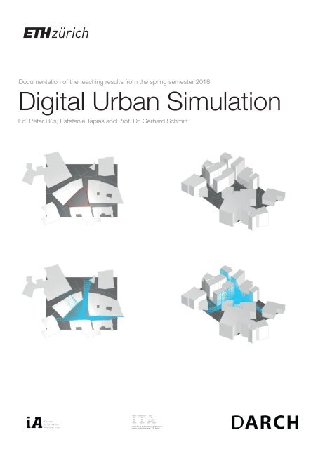
Digital Urban Simulation : Documentation of the Teaching Results from the Spring Semester 2018

ame: 

ate: 

Alexander Metche 

14.05.2018 

escription: 

roject DataFlow Field of View focuses on creating an interactive planning tool for urban designers and 

rchitects. I started to think about an all-round defi nition for a view analysis. At the Kerez-Studio SS2018 

he site was up in the hills of Zürich, almost without infrastructure or a dense urban playground. 

y motivation was basically to create something that shows how people can see my building from differnt 

perspectives: from the top of the hills, through the forest, from the city, from different positions on the 

Documentation of the teaching results from the spring semester 2018 

treets. 

Digital 

A general tool, that you 

Urban 

can use easily, without any 

Simulation 

grasshopper or rhino skills. Just have it. In fi rst 

nstance you only need to load OSM-File from Openstreetmap.com “Figure 1” and HGT-File from USGS 

For Topography where you are located with your OSM-File). It will automatically generate buildings, streets, 

outes, Ed. waterways Peter Bǔs, and Estefanie land use, Tapias forests and Prof. with Dr. trees Gerhard included. Schmitt All in 3D. In Exercise 3 I tried to make an 3D 

sovist out of a sphere what subtracts any objects which block the view. It wasn’t very optimized at this 

tate, so I wanted to improve it and create a more precise version.”Figure 3-4” 

FIGURE 1: TOPVIEW 

GENERATED CUT OUT FROM OSM 

AND CHOSEN STREET FOR ANALYSIS 

FIGURE 2: ISOMETRIC VIEW 

3D-MODELL INCLUDES TOPOGRAPHY, BUILDINGS, ROUTES, HIGH- 

WAYS, LANDUSE AND WATERWAYS 


ALL ROUTES CAN BE CHOOSE BY SLIDING ONE SINGLE SLIDER 

ALL ROUTES WERE DIVIDED INTO 10 STEPS 

FIGURE 4: ISOMETRIC 

SURFACES WILL GETTING A POINT GRID IF SEEN 

THE GRID IS LINKED THROUGH LINES TO THE POINT OF VIEW 

igital Urban Simulation | Final examination 

IN FIGURE 1-4 DENSE URBAN SCENARIO, OVERVIEW AND SHOW CASE

Chair of Information Architecture 

Digital Urban Simulation 

Documentation of teaching results 

Peter Bǔs, Estefania Tapias, and Gerhard Schmitt 


Teaching 

Peter Bǔs, Estefania Tapias, and Gerhard Schmitt 

Syllabi 

http://www.ia.arch.ethz.ch/category/teaching/fs2018-digital-urban-simulation/ 

Seminar 


Students 

Alexander Metche, Christian Guenther, Heidi Silvennoinen, Jin Li, Paco Bos, Guo Zifeng 

Published by 

Swiss Federal Institute of Technology in Zurich (ETHZ) 

Department of Architecture 

Institute of Technology in Architecture 


Wolfgang-Pauli-Strasse 27, HIT H 31.6 

8093 Zurich 

Switzerland 

Zurich, September 2018 

Layout 

Brigitte M. Clements 

Contact 

tapias@arch.ethz.ch | http://www.ia.arch.ethz.ch/tapias/ 

Cover picture: 

Front side: Data Flow - Field of View Analysis, Alexander Metche, 2018

Course Description and Program 

DIGITAL URBAN SIMULATION 

Mondays 14:00 - 18:00 

063-0604-00L | 2 ECTS* 


In this course students analyze architectural and urban design 

using current computational methods. Based on these analyses 

the effects of planning can be simulated and understood. An 

important focus of this course is the interpretation of the analysis 

and simulation results and the application of these corresponding 

methods in early planning phases. 

The students learn how the design and planning of cities can be 

evidence based by using scientific methods. The teaching unit 

conveys knowledge in state-of-the-art and emerging spatial 

analysis and simulation methods and equip students with skills 

in modern software systems. The course consists of lectures, 

associated exercises, workshops as well as of one integral 

project work. 











Introduction to the course 

Simulation of urban networks and morphologies growth 

Space Syntax I 

Space Syntax II 

Seminar Week 

Urban Climate I 

Urban Climate II 

Workshop: from analysis to design proposals 

Guest lecture 

Final consultations 


Final presentations 

Where 

HIT H 31.4 (Video wall) 

Supervision 

Dr. Estefania Tapias 

Dr. Peter Bus 

tapias@arch.ethz.ch 

bus@arch.ethz.ch 

Exercises 50% (documentations) 

Presentation 25% (project at the end) 

Written documentation 50% 

The most recent outline will be found on www.ia.arch.ethz.ch 

Prof. Dr. Gerhard Schmitt 


Information Science Lab 

Wolfgang-Pauli-Strasse 27, 8093 Zurich 

www.ia.arch.ethz.ch

Content 

Data Flow - Field of View Analysis 

Student: Alexander Metche 

Creation and Analysis of Virtual Spaces: 

A Study of Reflections 

Student: Christian Guenther 

p.9 

p.17 

Effect of New Development on Arbon’s Centre 

Student: Heidi Silvennoinen 

Neighbourhood Design in Suburban Tangier 

Student: Jin Li 

HIPV on HIB 

Students: Paco Bos 

p.25 

p.37 

p.47 

Factors Influencing House Prices 

Student: Guo Zifeng

Data Flow - Field of View Analysis 

Student: Alexander Metche

DataFlow - Field of View Analysis 

Name: 

Date: 



Name: 

Date: 



Description: 

Project DataFlow Field of View focuses on creating an interactive planning tool for urban designers and 

architects. I started to think about an all-round defi nition for a view analysis. At the Kerez-Studio SS2018 

the site was up in the hills of Zürich, almost without infrastructure or a dense urban playground. 

My motivation was basically to create something that shows how people can see my building from different 

perspectives: from the top of the hills, through the forest, from the city, from diff erent positions on the 

streets. A general tool, that you can use easily, without any grasshopper or rhino skills. Just have it. In fi rst 

instance you only need to load an OSM-File from Openstreetmap.com “Figure 1” and HGT-File from USGS 

(For Topography where you are located with your OSM-File). It will automatically generate buildings, streets, 

routes, waterways and land use, forests with trees included. All in 3D. In Exercise 3 I tried to make an 3D 

Isovist out of a sphere what subtracts any objects which block the view. It wasn’t very optimized at this 

state, so I wanted to improve it and create a more precise version.”Figure 3-4” 

Questions and integration: 

There isn’t a practical view analysis out there, so I decided to make my own one. The analysis can be helpful 

to avoid looks from the outside. The Results can be integrated easily into your design process. Just do 

a View Analysis with multi-views and place your schematic Design to it. How to make an invisible Building? 

I can imagine using the tool to get a better overview of what and where I can build a building in a city like 

Berlin to prevent overpopulated cities, by making the Buildings “Invisible”. 

I used and tested a few View of Field analyses. For Example, the Ladybug Spatial Analysis “Figure 5-8”, 

what can give out information’s about what’s seen and unseen in a percentage. Unfortunately, it’s not that 

precise and you can’t see all the views as lines for a better understanding. Its only based on colours and 

was integrated into the Tool. 


GENERATED CUT OUT FROM OSM 

AND CHOSEN STREET FOR ANALYSIS 



WAYS, LANDUSE AND WATERWAYS 


LADYBUGS VIEWANALYSIS 


OVERLAPPING LADYBUGS VIEW-ANALYSIS WITH THE POINT GRID FROM 

THE DATAFLOW FIELD OF VIEW 


ALL ROUTES CAN BE CHOOSE BY SLIDING ONE SINGLE SLIDER 

ALL ROUTES WERE DIVIDED INTO 10 STEPS 


SURFACES WILL GETTING A POINT GRID IF SEEN 

THE GRID IS LINKED THROUGH LINES TO THE POINT OF VIEW 

FIGURE 7: STATISTIC INTERFACE 

FIRST ONE FROM TOP TO BOTTOM VISIBLE FACADE IN % LADYBUG 

8.46 % 

SECOND ONE VISIBLE FACADE IN % FIELD OF VIEW 

9.58 % 


BLACK CONTOUR SHOWS THAT LADYBUG STILL HAS ISSUES IN VIEW- 

ING EXACT RESULTS 

Digital Urban Simulation | Final examination 

IN FIGURE 1-4 DENSE URBAN SCENARIO, OVERVIEW AND SHOW CASE 


IN FIGURE 5-8 COMPARISON BETWEEN DATAFLOW FIELD OF VIEW AND LADYBUGS VIEWANALYSIS 

10 New Methods in Digital Urban Simulation | Final project documentation 

New Methods in Digital Urban Simulation | Final project documentation 11

Name: 

Date: 



Name: 

Date: 



How it works: 

All Data are generated through OpenStreetMap Information’s. The 3D-Modell includes all necessary information’s 

from Buildings up to Highways and Topography. The tool creates invisible points on all surfaces 

on all objects. The Point of View can be selected on each street, highway or route that shows up and is 

divided into 10 steps each. The Field of View tool will also like the Sphere Isovist subtract any object which 

Block the View. Because of only lines and points the performance and results are much higher. I coupled 

the Ladybug view analysis with the tool, to see the exact difference in visual and in statistics. For the outcome 

of what is the percentage of visible surfaces in correlation the clipped cut out from OSM and the min 

and max length of each view thread, I used Human UI, what will give me a live ticker information window 

about the current situation. 

Conclusion Digital Urban Simulation: 

All analyses I did at this department where interesting for different kind of Situation in a development process. 

But I think in the end every analysis must be rewritten for a specifi c Problem or Project. In Exercise 

3 I mentioned that’s irrelevant to have the shortest path, when the path is quite cliffy, so I searched for that 

specifi c Issue and build up an Ivy grid to get the shortest path in height and not in length. 

I never worked with Grasshopper that intense and think that through this new experience in parametric 

design and analyses, I will automatically think different when I start a project. 


ANOTHER CUTOUT GENERATED 

LESS DENSE/URBAN MORE NATURE VIEW 



WAYS, LANDUSE (TREES) AND WATERWAYS 


OVERLAPPING OF 5 POINTS OF VIEW FROM THE CENTER 


DECISION IS NOW POSSIBLE WHERE TO ADD BUILDINGS TO SHOW OR 

TO HIDE 


LESS POINTGRID IS USED TO AVOID PERFORMANCE ISSUES 

FROM WHERE ON THE ROUTE IS THE LANDSCAPE VISIBLE 


BLACK COLUMNS/TREES ARE DETECTED 

BY THE DATA FLOW FIELD OF VIEW 


LANDSCAPE POSSIBLE VIEWS LONGSTREET 

OVERLAPPING OF 4 POINTS OF VIEW 


OVERLAPPING INDICATES POSSIBLE LOCATIONS AND GAPS IN VIEW 


IN FIGURE 9-12 LANDSCAPE SCENARIO, OVERVIEW AND SHOWCASE 


IN FIGURE 13-16 OVERLAPPING STRUCTURES FOR MORE EFFICENT DECISION-MAKING 



Name: Alexander Metche 

Date: 14.05.2018 

GENERATING HIGHWAYS AND 

ROUTES 

SELECTING ROUTES OR HIGH- 

WAYS AND DIVIDING THE CURVE 

INTO SEVERAL STEPS 

POINT OF VIEW UP TO 2 METERS 

INPUT OSM FROM 

OPENSTREETMAP 

GENERATING FOREST 

PROJECTING BUILDINGS COR- 

RECTLY TO THE SURFACE OF THE 

TOPOGRAPHY 

FOR MORE ACCURACY 

USE MERRKAT WITH GIS DATA 

INPUT HGT FROM USGS 

GENERATING TOPOG- 

RAPHY 

GENERATING BUILDINGS 

HEIGHT ACCORDINGLY CHOSEN 

BY THE ORIGINAL HEIGTHS FROM 

GEO.ADMIN.COM 

BUILDINGCOUNTER IN 

THE CONTEXT 

(HOW MANY BUILDINGS 

ARE IN THE SEROUND- 

ING) 

LANDUSE BOUND- 

RIE-LINES ACCURATELY 

PROJECTING TO TO- 

POGRAPHY 

GENERATING TREES 

IN FORM OF BLACK 

COLUMNS (CAN ALSO 

BE DONE WITH PROXY 

SHATTER AND VRAY 

TREES) 

HUMAN UI INTERFACE TO 

SHOW ALL INTEGRATED 

STATISTICS 

DATAFLOW FIELD OF 

VIEW ANALYSIS - DEFI- 

NITION 

MIN. AND MAX. VIEW-LENGTH 

INTEGRATED LADYBUG 

VIEWANALYSIS FOR BETTER 

UNDERSTANDING 

MATH VISIBLE FACADE IN % IN 

CORRELATION TO THE WHOLE 

CUT-OUT 

MOST ACCURATE CONFIG FOR 

COLORING THE VISIBLE VIEW 

VISIBLE FACACE IN % (LADY- 

BUG) 



Creation and Analysis of Virtual Spaces: 

A Study of Reflections 

Student: Christian Guenther

Creation and Analysis of Virtual Spaces: A Study of Reflections 

Final Examination 

Name: Christian Guenthner 

Date: 13 th May 2018 

Summary: 

In this project, a generalization of the isovist analysis is proposed to study the impact of reflective surfaces on the viewable 

area of an observer. To this end, the concept of virtual spaces is introduced, where mirrors serve as “windows” into a 

mirrored world. Isovist viewfields are calculated for visualization and quantification purposes. Common view properties such 

as viewable area, perimeter, and compactness can be determined and allow for the quantification of spaces in the presence 

of planar reflective surfaces. Finally, a simple extension of the algorithm to non‐planar reflective surfaces, such as convex 

mirrors, is proposed. The algorithm is employed to study the effect on the isovist of an exemplary building layout in first, the 

presence of planar mirrors, second a mirror of variable size, and third a parameterized parabolic mirror undergoing the 

transition from concave to convex. While the extension is demonstrated in the context of a room, it further allows to study 

view fields in an urban context including reflective façades. 

Motivation: The quantification of view fields is key for the understanding of visual properties of spaces. To this end, 

the isovist is determined, which contains all points that can be seen from the position of an observer [1]. The 

DeCodingSpaces toolbox [2], a plugin for Grasshopper[3] & Rhino3D[4], allows to determine these isovist fields for 

arbitrary 2D geometries. With the advent of huge glass or polished metal façades or reflective water bodies into 

modern architectural design [e.g. 5], the impact of reflective surfaces on the isovist becomes important. Hence, this 

project aims to propose a generalization of the isovist component to analyse the impact of mirrors on view fields. 

To determine the mirror view, a virtual space is constructed. Starting from the room layout, a planar mirror is 

selected. An infinite mirror surface is used to first, cull the room behind the mirror and then reflect the remaining 

geometry, creating the virtual space. The mirror serves as a window to this space by introducing view blocking walls 

to the left and right of the mirror. After removing the mirror from the combined room and virtual space geometry, 

an isovist calculation can be applied again to determine the observer’s view into the virtual space. Mirroring and 

culling the view at the selected mirror surface leads to the final mirror view. Combining the view from both isovist 

calculations creates the actual view perceived by an observer. 

Quantification of Reflections: In order to quantify view properties, the outputs of three isovist components can be 

combined as follows (Figure 2). Both direct view and the view into the virtual space are calculated in the same 

manner as before. In order to compensate for the view field between the observer and the mirror, a third isovist 

calculation is performed on the combined space, where the mirror is replaced by a wall. The respective view 

property of the mirror view is given by the difference of the “view to mirror”‐ and the “view into the virtual space” 

values. This calculation assumes linearity of the view property, which is given e.g. for viewable area or perimeter. 

The calculation of a non‐linear property such as compactness must be based on the culled reflected view field as 

determined above. 

Theoretical Concept: In order to calculate view properties in the presence of mirrors, the viewable area is 

decomposed into two groups (see Figure 1): (a) direct view, i.e. the viewable area without reflections, and (b) a 

mirror view. The direct view is calculated using a standard isovist simulation. 

Figure 1: Conceptual drawing of the combined isovist calculation for the “direct view” and the “mirror view” through a virtual space. 

Digital Urban Simulation | Creation and Analysis of Virtual Spaces: A Study of Reflections 

Figure 2: Three isovist calculations are used to determine the area of the view field using the concept of the virtual space. By replacing the window 

to the virtual space by a wall in a third isovist calculation, the view area of the mirror space can be determined by subtraction. In this way, the 

complex culling operation of the view field can be avoided accelerating the quantification of the view. This technique can be used for any linear 

view properties, such as viewable area or perimeter. 

Reflection Study – Single Mirror: In Figure 3, the resulting viewable area, perimeter, and compactness are 

displayed for the above case of a single angulated mirror. Here, both area and perimeter are approximately doubled 

by the presence of the mirror leaving the compactness of the space nearly unchanged. This can be understood as an 

opening of the view creating the perception of a wider space while maintain the view complexity. 




Figure 5: Change in viewable area as a function of the mirror size from no mirror to full‐sized mirror. Especially the center room with only reduced 

view of the outside benefits from the full‐sized mirror. 25% wall‐coverage suffices to increase the left room’s visible area to its maximum value. 

Figure 3: Comparison of viewable area, perimeter, and compactness for direct, mirror, and combined view in the presence of a single mirror. Here, 

the mirror approximately doubles the viewable area, while compactness of the space is only slightly reduced. 

In Figure 4, a grid analysis of the three view parameters is given comparing the view with and without an additional 

planar mirror. The addition of the mirror leads to an increase in both area and perimeter, while compactness is 

reduced. While the large planar mirror again opens the space, it also reduces compactness due to the complexity of 

the reflected view field. 

Reflection Study – Curved Mirrors: So far, only planar mirror surfaces have been studied. Typically, these surfaces 

increase the viewable area considerably with only minor impact on the compactness of the space. A curved 

reflective surface can be approximated by decomposing it into multiple planar mirrors (Figure 6). In this study, a 

parabolic mirror was parameterized allowing it to be changed from concave to convex. For the concave mirror, the 

focal spot lies in front of the mirror. Hence, all building elements residing behind the focal spot are seen inverted 

(case 1) and elements between the mirror and twice the focal distance are seen magnified. Concave mirrors 

typically lead to reflections, which are difficult to grasp. Convex mirrors on the other hand allow to increase the 

viewable area beyond the capabilities of a planar mirror and are hence often used for passenger‐side mirrors in cars 

or on road‐sides to reduce blind spots. 

Figure 6: Construction and comparison of a parametrized parabolic mirror as it transforms from concave to convex. The bend mirror surface is 

approximated by 25 planar mirrors. For the concave mirrors, effects like the focal spot and inversion of the viewable image can be observed, while 

convex mirrors lead to a widening of the viewable area. N.B.: The discrete reflected view fields in all four cases are an artifact of the discretization 

of the mirror. The actual view field of a continuously bend parabolic mirror is continuous itself. 

Figure 4: Grid analysis of the viewable area, perimeter, and compactness of the same space with and without a planar mirror (green) assuming a 

360° view angle in each cell. The addition of the mirror leads to an increase in viewable area, as well as, perimeter again leading to the perception 

of a wider space. At the same time, compactness is greatly reduced in the center of the space due to the increased complexity of the mirrored view 

field. 

Reflection Study – The Growing Mirror: In a second reflection study, the above planar mirror is grown from left to 

right (Figure 5). Here, the full‐sized mirror is especially useful to improve the visible area in the center room, which 

benefits from views of both the left and the right room. The maximal viewable area in the left room is already 

achieved with as little as 25% wall coverage. 


Limitations: The ansatz of virtual spaces for the determination of view fields in the presence of reflective surfaces 

poses some limitations, which shall be briefly addressed here. First, the decomposition of curved reflective surfaces 

into piecewise planar mirrors is numerically unstable as the mirror size reduces drastically and hence the accuracy of 

the isovist component needs to be increased. This can already be observed in Figure 6, where the view fields of 

adjacent mirror surfaces already slightly overlap. Second, the discretization of the continuous bend surface leads to 

a discrete set of mirror views. However, the view field of a continuous mirror is continuous itself. Thus, a 

quantitative analysis of the reflections in the presence of curved mirrors is not advisable with this method. Third, 

even though multiple reflective surfaces can be easily simulated and combined, multiple reflections are neglected 

here. While the concept of virtual spaces can be applied to multiple reflections as well, the implementation in 

Grasshopper is not straight forward. To overcome all draw backs, a ray‐based analysis taking reflection laws into 

account might be favoured over the virtual space concept. The latter, however, provides an easy and more intuitive 

understanding of reflections. 

Conclusions: In this project, an extension of the isovist was proposed that allows to take reflective surfaces into 

account. To that end, the mirror is seen as a window into a virtual space. This space can be analysed equivalently as 

a direct view that does not contain reflections. While reflective surfaces within the view field always increase the 

viewable area, close attention has to be paid with regards to increased complexity of the reflected space. As a rule 

of thumb, single, planar reflective surfaces typically do not impact the complexity of the view field and are 




into piecewise planar mirrors is numerically unstable as the mirror size reduces drastically and hence the accuracy of 

the isovist component needs to be increased. This can already be observed in Figure 6, where the view fields of 

adjacent mirror surfaces already slightly overlap. Second, the discretization of the continuous bend surface leads to 

a discrete set of mirror views. However, the view field of a continuous mirror is continuous itself. Thus, a 

quantitative analysis of the reflections in the presence of curved mirrors is not advisable with this method. Third, 

even though multiple reflective surfaces can be easily simulated and combined, multiple reflections are neglected 

here. While the concept of virtual spaces can be applied to multiple reflections as well, the implementation in 

Grasshopper is not straight forward. To overcome all draw backs, a ray‐based analysis taking reflection laws into 

account might be favoured over the virtual space concept. The latter, however, provides an easy and more intuitive 

understanding of reflections. 

Conclusions: In this project, an extension of the isovist was proposed that allows to take reflective surfaces into 

account. To that end, the mirror is seen as a window into a virtual space. This space can be analysed equivalently as 

a direct view that does not contain reflections. While reflective surfaces within the view field always increase the 

viewable area, close attention has to be paid with regards to increased complexity of the reflected space. As a rule 

of thumb, single, planar reflective surfaces typically do not impact the complexity of the view field and are 

Digital perceived Urban as opening Simulation the | space. Creation Convex and mirrors Analysis can of Virtual be used Spaces: to increase A Study the of viewable Reflections area beyond the capabilities of 

a simple planar mirror and are easy to comprehend. On the other hand, concave reflective surfaces as well as 

multiple reflections (not studied here) lead to increased view complexity and are typically hard to grasp. 

References: 

[1] M L Benedikt, To Take Hold of Space: Isovists and Isovist Fields.Environment and Planning B, 1979; 6 (1): 47‐65 

[2] DeCodingSpaces (v2018.01) http://decodingspaces‐toolbox.org/ 

[3] Grasshopper (v1.0.0005) http://www.grasshopper3d.com/ 

[4] Rhinoceros 6, https://www.rhino3d.com/ 

[5] Mirror Houses (Architect: Peter Pichler), http://www.peterpichler.eu/mirror‐houses/, Accessed: 05/13/2018 



Effect of New Development on Arbon’s Centre 

Student: Heidi Silvennoinen

EFFECT OF NEW DEVELOPMENT ON ARBON’S CENTRE 

Name: 

Date: 

Heidi Silvennoinen 


1. Summary 

The redevelopment of Arbon is a project for Prof Caruso’s Ideal City Studio this semester. My task for the studio 

is to apply Renaissance city planning ideals to Arbon, a small town in North-Eastern Switzerland. In the status 

quo, the site is largely empty with some industrial warehouses, a nice lakeside path, a train station and some 

residential and commercial buildings (Fig. 1). The site is located beside a local shopping street and it is within 

walking distance of Arbon’s cultural and historical centre. The aim of this research is to find out what impact 

the new development has on Arbon’s centre: will it become the new centre of Arbon or will the old centre 

maintain its vitality? 

Fig 2. Palmanova, an example of a highly centralised Renaissance city with a central plaza. 

Industrial buildings 

Train station 

Central plaza 

2. Motivation: 

The question of centrality is especially interesting given that the new development is inspired by Renaissance 

urban planning ideals. Renaissance ideal cities were almost always highly centralised, often circular 

in form with streets radiating outward from a single centre (Fig. 2). In the centre there was generally a 

plaza surrounded by the most important buildings and institutions of the city. Renaissance main plazas 

were central both in terms of access to other buildings in the city (since they were located in the physical 

centre of a symmetrical city) and in terms of access to points of interest (since the plaza was surrounded 

by the most important buildings). 

Shopping street 

Historical centre 

Our design for Arbon is also focused on a central plaza. It is interesting to investigate whether our plaza 

will become the centre of the city in the same way that Renaissance plazas were. City graph analyses can 

help evaluate whether our plaza is truly a Renaissance-style central plaza. 

Fig 1 a). Arbon in status quo with site highlighted. 

Fig 1 b) New development on site. 

3. Analyses and Interpretation 

The impact of our proposed development on Arbon’s centre is investigated in two ways: 1) whether the 

plaza is a centre in terms of access to gross area of all other buildings in Arbon and 2) whether the plaza 

is a centre in terms of access to interesting locations in the city, such as libraries, shops and restaurants. 

Weighted closeness centrality is used for both analyses. The idea is to find out which streets are important, 

and the importance is assigned by the closeness of the street to important destinations in the city. 

3.1. Centrality in terms of access to maximum gross area 

Digital Urban Simulation | 

Final examination 

It is assumed that the more gross area a building has, the more people live and work there and therefore 

move near the building. A key aspect of centrality is being located in a place where lots of other people 

are. In order to measure a street’s centrality, it is therefore interesting to know how well connected that 

street is to all the gross area of the surrounding city’s buildings. 

The input data required for this calculation consist of: 2D outlines of building footprints, 2D road network 

and a 3D model of all buildings in the city. The first two requirements were fulfilled by a simple DWG file 

while the 3D model for Arbon was obtained from SwissTopo. 



The gross area of each building was calculated by first finding the area center of each building footprint. 

This center point was then projected upwards as a ray until it intersected with the 3D building mesh. A 

line was drawn upward from the first intersection point with the mesh until a second intersection, thereby 

giving the height of the building. Gross area was then estimated by dividing the building height by 3 

(a typical storey height) and multiplying this number of stories by the building footprint’s area (Fig. 3). 

Fig 4 a) Weights of buildings by gross area in status quo 

Fig 3. Input data and method for extracting the gross area of each building. 

Each building in the city was then given a weight proportional to its gross area. The weights are represented 

as circles in Fig 4 a-b) and the resulting closeness centrality analysis is shown in Fig 5 a-b). The 

analysis shows that the plaza does not become a centre in terms of access to buildings’ gross area although 

it obviously increases the centrality of the site which is largely empty in the status quo. In order to make 

the plaza more central, buildings adjacent to it or South of it should be made denser. 

Fig 4 b) Weights of buildings by gross area in new development. 



0-20 percentile 

21-40 

41-60 

61-80 

81-100 

3.2. Centrality in terms of access to points of interest 

Even if a street is near buildings with massive gross area, another street near smaller but more interesting 

buildings might have more people visiting it. It is therefore necessary to evaluate the centrality of Arbon’s 

new development in terms of access to points of interest. 

In this analysis it was first necessary to assign points of interest to the map of Arbon in both the status 

quo and the new plan. Points of interest were determined by closely examining the Google map of 

Arbon, which contains tags for shops, services and other points of interest in the area. Point objects were 

placed on the Rhinoceros map of Arbon on each real-life point of interest. Different categories of points 

were assigned weights based on how often they are generally frequented by a person. For example 

supermarkets were given a weight of 4 while restaurants were only given a weight of 1 since most people 

frequent the former much more often than the latter. 

Fig 5 a) Centrality measured by access to gross area, status quo. 

The weights of the status quo were copied to the new plan unless the point was located inside the 

redevelopment site. Points of interest were added to the proposed new buildings according to their 

prospective function. The points of interest are shown in Fig 6 a-b). The weighted closeness centrality 

analysis based on these points of interest is shown in Fig 7. The analysis shows that the Northern part 

of the new development has better access to points of interest compared to the plaza. In order to make 

the plaza more interesting, the amount of points of interest adjacent to it or on its southern side should be 

increased. 

Fig 5 b) Centrality measured by access to gross area, new development. 



Train station (weight 10) 

School / day care (4) 

Shop (1) 

Supermarket (4) 

Recreation / sports (2) 

Art / culture (2) 

Restaurant (1) 

0-20 percentile 

21-40 

41-60 

61-80 

81-100 

Fig 6 a) Weights of points of interest in status quo. 

Fig 7 a) Centrality measured by access to points of interest, status quo. 

Fig 6 a) Weights of points of interest in status quo. 

Fig 6 b) Weights of points of interest in new development. 

Fig 7 b) Centrality measured by access to points of interest, new development. 



4. Conclusion 

The analyses show that in its current form, the new plaza does not form an unequivocal centre for Arbon 

in terms of access to gross floor area or points of interest. The new plan does decrease the centrality of 

the historic centre, moving Arbon’s centre towards the shopping street at the Northern end of the development 

site. If the goal is to make the new plaza a true focal point of Arbon, the analysis shows that the 

building density and points of interest near the plaza should be increased. 



Neighbourhood Design in Suburban Tangier 

Student: Jin Li

Motivation 

1) Better understand the urban network of the site, in the city of Tangier, with Rhino Grasshopper parametric 

tools; 

2) Analyse the self - constructed houses with Ladybug to optimize housing design and make proposals to local 

residents. 

Network Analysis 

1.5km 

1.5km 

1.0km 

1.0km 

0.5km 

Existing Network Choice Analysis 

0.5km 

0km 

0km 0.5km 1.0km 

In recent years Tangier,Morocco has been subjected to strong migratory movements from both foreign 

and rural regions, intensely pressuring its built capacity. Non-regulated houses were built with expanding 

of the city. 

The project is situated in the north west Tangier suburban area,5km from the city center between an unregulated 

area 0km and an upper class neighborhood, 0.5km called “California”.There is an 1.0km ongoing project on site that 

consists of apartment buildings and villas. 

0km 

In recent years Tangier,Morocco has been subjected to strong migratory movements from both foreign 

and rural regions, intensely pressuring its built capacity. Non-regulated houses were built with expanding 

of the city. 

The project is situated in the north west Tangier suburban area,5km from the city center between an unregulated 

area and an upper class neighborhood, called “California”.There is an ongoing project on site that 

consists of apartment buildings and villas. 

Existing Network Integration Analysis 



MAS UD 

Proposal Network Choice Analysis 

Proposal Network Integration Analysis 

Choice Analysis Defination 

Integration Analysis Defination 

Proposed Network 



Housing Typologies 

To control the incremental expansion, we create a module of 18 by 18m divided into a grid of 3.60 by 3.60m, which can be used by two to four 

families depending to their income. The divisions of the grid can be a solid or a void functioning as a room or a courtyard accordingly. The 

house units are built with self built techniques already used in the unregulated area. 

Isovist Analysis of the open space 

Defination 



Radiation Analysis of Proposed Typologies 

Sun Paths and Shadows of Housing Units 

Defination 

Defination 



BIPV on HIB 

Student: Paco Bos

Name: Paco Bos 

Date: 19-05-2018 

Summary: 

The HIB building on the Hönggerberg campus overheats. Therefore, a shading system will be designed. 

The goal of this project is to find an angle for the shading system that maximizes the irradiation on the 

shading surface. The second step is to minimize the cooling and heating load inside the building. Last, 

the level of self-sufficiency will be assessed. Figure 1 shows the flow of data that should achieve these 

goals. 

Analysis 1 (angle optimization): 

The first step in the process is to maximize the energy generation. To achieve this, the solar irradiation 

must be maximized. After assuming a usable fraction of the area and total system efficiency of 

respectively 0.9 and 0.18, the usable electricity can be calculated. Figure 3 shows the yearly generated 

electrical energy as function of the angle (a horizontal surface has an angle of zero degrees). The optimal 

angle was found to be 28 degrees down from the horizontal. 

Figure 1: Data flow overview 

Electric energy generated (kWh/y) 

1946 

1944 

1942 

1940 

1938 

1936 

1934 

Motivation: 

The HIB building on the Hönggerberg campus overheats in summer. Especially rooms oriented to the 

south have issues regarding thermal comfort. In my semester project I focus on the part of thermal 

comfort by assessing the influence of different shading systems. I realized that it is possible to add solar 

panels to this shading system. This way, energy can be generated at the same time the cooling load is 

reduced. Thus, this project will focus on the energy consumption and generation of the HIB building. The 

main part of the building consists of a large open space. This is very hard to simulate accurately with the 

program that is used. Next to that, the main issue of overheating occurs on the south side. Therefore, 

only room HIB E 11 will be simulated. 

1932 

25 26 27 28 29 30 31 32 33 34 35 

Angle downward from horizontal (degree) 

Figure 3: Finding the angle for maximal energy generation 

Analysis 2 (height optimization): 

The second step is to lower the energy demand. This is done by adjusting the height of the shading 

system while keeping the angle fixed to 28 degrees. Figure 6 shows the yearly heating and cooling 

demand as the height of attachment of the shading system is adjusted. A height of 0 m indicates that 

the shading system is attached at floor height and at 2.9 m that it is attached at ceiling height. Although 

the total load between 2.2 and 2.9 m does not vary much, the very minimum can be found at 2.6 m. 

Another thing that becomes clear immediately, is how the cooling load dominates the thermal energy 

load. 

Digital Urban Simulation | BIPV on HIB 

Energy demand (kWh/y) 

20000 

18000 

16000 

14000 

12000 

10000 

8000 

6000 

4000 

2000 

0 

0 0.2 0.4 0.6 0.8 1 1.2 1.4 1.6 1.8 2 2.2 2.4 2.6 2.8 

Height of shading (m) 

Heating 

Cooling 

Figure 2: Finding height of shading system for minimal energy demand 


Digital Urban Simulation New Methods | Name in of Digital the project Urban Simulation | Final project documentation 49

Analysis 3 (self-sufficiency): 

Now that the energy generation is maximized and the load minimized, we can zoom in to see monthly 

values and compare the status quo to the situation with the shading system as defined in earlier stages 

(i.e. with an angle of 28 degrees and a height of 2.6 m). Figure 4 shows only the cooling demand, 

because the heating demand is neglectable (see Figure 2). The effect of the shading system becomes 

clear: during all months of the year the demand is reduced, and the yearly demand is flattened. 

Energy demanded (kWh) 

2500 

2000 

1500 

1000 

500 

Self-sufficiency light and cool (%) 

120 

100 

80 

60 

40 

20 

0 

1 2 3 4 5 6 7 8 9 10 11 12 

Time (months) 

Light Cool 

Figure 5: Self-Sufficiency adjusted for heat 

0 

1 2 3 4 5 6 7 8 9 10 11 12 

Cool with shading 

Time (months) 

Cool without shading 

Figure 4: Cooling energy demanded with and without shading 

The final assessment regards the self-sufficiency, which is a ratio of directly consumed energy and 

energy demanded. For the sake of simplicity, it is assumed that all generated energy can be consumed 

immediately. This might not be too far off when the building is connected to the district heating system 

of the campus. 

To convert the electrical energy to heating and cooling energy, a heat pump COP of respectively 7 and 4 

is assumed. Figure 5 shows the self-sufficiency. This is adjusted to the case where all energy is first 

consumed to supply the heating demand, because this demand can be covered year-round. All energy 

that is left can be fully converted to supply the cooling demand or be directly used to supply the lighting 

load. After covering the heating demand, the cooling demand can be covered for roughly 50 to 60 %. It 

is important to note that these demand profiles only apply to the one room that has been modelled. 

Other rooms will receive less irradiation and might have a similar total energy demand. Therefore, the 

numbers shown, can be interpreted as maximum level of self-sufficiency. 

Conclusions: 

The shading system that is created, is more than just a shading system that reduces the cooling load. It is 

also a source of energy. Although not assessed, daylighting might be influenced relatively positive due to 

the small gap between the top of the shading and the top of the window (see Figure 6). If the shading 

system were to be attached to the very top, less natural light would be received at the back of the room. 

Furthermore, this simple design allows for a reasonable self-sufficiency for this single room. 

Additional geometries can be tested. For example, a vertical slab is likely to be adequate on the western 

façade. Also a geometry that is better corresponding to the geometry of the roof could be tested so that 

a more architecturally sound design is created. Lastly, a dynamic shading system could be modelled. 

Figure 6: Final position of the shading system 

50Digital Urban New Simulation Methods | in Name Digital of Urban the project Simulation | Final project documentation 


Appendix: 

Figure 7: Grasshopper definition 



Invisible Architecture 

Student: Guo Zifeng









Chair of 

Information 

Architecture

Digital Urban Simulation : Documentation of the Teaching Results from the Spring Semester 2018

Create successful ePaper yourself

Delete template?

Save as template?