Exploring Earth's Magnetic Field - Three make a SWARM

INTERNATIONAL
SPACE
SCIENCE
INSTITUTE
SPATIUM
Published by the Association Pro ISSI No. 43, June 2019

Editorial
Even if you are neither a migrating
bird nor a seafarer nor any kind of
navigator you might have at least
wondered how the majority of
these species are able to follow their
paths and reach their far-away
destinations on our planet. Concerning
bird migration – this
phenomenon employs a variety of
senses, using, for example, landmarks
and the Sun as orientation.
However, a large part of the orientation
guidance can be ascribed to
the magnetic field of the Earth.
Not only birds, but also various
other animals use magnetoreception,
the ability to detect magnetic
fields, for orientation. How exactly
this works, is not quite clear yet. It
is hypothesised that proteins harbouring
magnetically sensitive
radical pairs (“magnetic molecules”)
are responsible. Iron-containing
minerals could also be
involved, which have, for example,
been detected in proteins found in
pigeon beaks.
If, however, you lack a significant
amount of magnetically sensitive
proteins and do not enjoy looking
at a compass and map, and prefer
navigation with electronic devices
like phones and handheld computers,
you should still be aware that
the smartphone also commonly relies
on a model of the geomagnetic
field to determine your heading.
There are many more life-sustaining
features connected with the
magnetic field of the Earth, but in
particular its navigation support is
gratefully acknowledged by the
biased editor.
In the preceding issues of Spatium
we studied the puzzles of fellow
Solar System planets such as Jupiter
and Saturn, their structure and
cores – it is time to wonder about
the home station again … Earth
still holds more than enough secrets
for us to unravel. Some of
them can be well addressed from
space, and the magnetic field of our
planet belongs to those.
In March 2019, Prof. Nils Olsen
from the Technical University of
Denmark gave an excellent presentation
on the geomagnetic field
and its study in the pro ISSI lecture
series. In this Spatium, we thus take
the opportunity to introduce this
fascinating topic.
Anuschka Pauluhn
Mönthal, June 2019
Impressum
ISSN 2297–5888 (Print)
ISSN 2297–590X (Online)
Spatium
Published by the
Association Pro ISSI
Association Pro ISSI
Hallerstrasse 6, CH-3012 Bern
Phone +41 (0)31 631 48 96
see
www.issibern.ch/pro-issi.html
for the whole Spatium series
President
Prof. Adrian Jäggi,
University of Bern
Layout and Publisher
Dr. Anuschka Pauluhn
CH-5237 Mönthal
Printing
Stämpf li AG
CH-3001 Bern
left: Nautical Chart of Mustique Island, Grenadines, Caribbean. On the right side
the compass rose is shown referencing the difference of compass reading and true
geographic north (declination). Credit: US National Geospatial-Intelligence Agency.
right: Heading on a sailing tour from Tromsø to Svalbard.
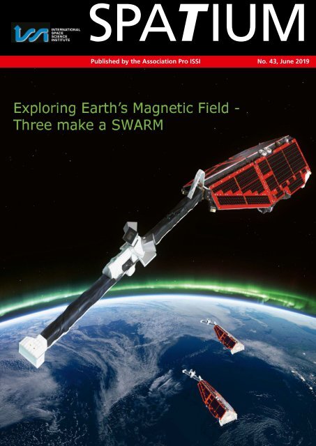
Title Caption
Swarm over the Earth.
Artist’s impression based on the true
design of the spacecraft.
Credit: ESA/AOES Medialab.
SPATIUM 43 2

Exploring Earth’s magnetic field –
Three make a Swarm 1
Nils Olsen, DTU Space – Technical University of Denmark and Anuschka Pauluhn, PSI Villigen
Introduction
It is amazing how many important
aspects of great impact in our
every day life are still largely enigmatic
to us. The Earth’s magnetic
field is a good example – it belongs
to the most mysterious aspects of
our habitat. Indeed, the electromagnetic
field in and around Earth
generates complex forces that have
innumerable effects on our daily
environment and life.
The geomagnetic field provides a
huge shield that protects us from
harmful solar charged particles and
cosmic rays. Without this protection,
life in its current form would
not exist. Although it might not
appear so at first glance, the Earth’s
magnetic field is permanently
changing: the magnetic north pole
wanders – currently several tens of
kilometres per year – and every few
hundred thousand years the polarity
of the Earth’s magnetic field
flips. The field strength is constantly
changing too – at present
significantly weakening. Over the
last 100 years, the dipole part alone
has decreased by 7 %. However, in
certain areas on Earth, for instance
in the Southern Atlantic, the weakening
of the geomagnetic field is
even stronger. Since this is the region
of lowest field intensity on
Earth, any further weakening is of
particular concern.
The geomagnetic field extends
from Earth’s interior out into space
where it interacts with the solar
wind, the stream of charged particles
emitted by the Sun. Most of
the Earth’s magnetic field is
thought to be generated by an
ocean of liquid iron that makes up
Earth’s outer core, 2 900 km under
our feet – there, temperatures are
about 4 500 °C, so that the molten
iron resembles the viscosity of water.
Acting like the spinning conductor
in a bicycle dynamo, this
“geodynamo” generates electric
currents and thus the continuously
changing electromagnetic field 2 .
However, our understanding of
how exactly the Earth’s dynamo
works and why it changes is still
very limited. For example, computer
models that reproduce some
of its features have only been developed
in the last few decades.
Not only the Earth’s core contributes
to the geomagnetic field,
other sources of magnetism are
magnetised rocks in the Earth’s
crust, with the ionosphere, the
magnetosphere and even the
oceans also playing a role. The resulting
field is a superposition of all
these effects. It is thus a major task
to observe and measure the complex
and constantly changing geomagnetic
field as precisely as possible
in order to advance many
areas of Earth science. In addition
to terrestrial observations, highly
accurate and frequent measurements
of the magnetic field from
space can provide new insight into
our planet’s formation, dynamics
and the entire environment stretching
from the Earth’s core to outer
space.
Figure 1: Artist’s rendition of Earth’s magnetosphere (not to scale, credit: NASA).
1
The current issue of Spatium has been drafted by Dr. Anuschka Pauluhn, based on a seminar by Prof. Nils Olsen
on March 27, 2019 in the pro ISSI series. Support from Prof. Martin C. E. Huber and Dr. Andreas Verdun is gratefully
acknowledged.
2
The term electromagnetic here is used to describe the fields generated by varying currents rather than electromagnetic
wave (AC) phenomena, thus it refers to currents and permanent magnetic fields.
SPATIUM 43 3

The first space missions to measure
the terrestrial magnetic field
were launched in the 1960s, but
they measured only its magnitude,
not its direction. After the brief
lifetime of the Magsat mission
(7 months in 1979 and 1980),
which carried the first space-borne
high-precision vector magnetometer,
the Danish Ørsted satellite
measured the magnetic vector field
for more than 15 years from 1999.
The German CHAMP mission
continued to do so from 2000 to
2010.
In 2000, ESA launched the Cluster
mission to measure the field
farther out: four satellites to study
the interaction of the solar wind
with Earth’s own magnetic field
that creates the terrestrial magnetosphere
(see also Spatium 9 by
G. Paschmann). The Cluster satellites
are relatively far from Earth in
elliptical orbits ranging from
19 000 km to 119 000 km. ESA’s
more recent task force investigating
the Earth’s magnetic field, the
constellation of the Swarm satellites,
continues the work started by
Ørsted and CHAMP. Launched in
2013, the three Swarm satellites
operate much closer to Earth than
Cluster, at a maximum distance of
around 500 km. The two missions
thus collect complementary data
on a quantity that is of paramount
importance for a variety of studies
related to our planet – the geomagnetic
field.
Figure 2: Earth’s magnetosphere. All that can be studied from Cluster to Swarm.
(Credit: NASA).
Some magnetic reference data for comparison:
The magnetic field of a small bar magnet (like “refrigerator” souvenir
magnets) at a short distance of about 1 cm: 0.01 T.
The bending magnet (dipole) field in an electron accelerator (on an
axis of the machine, which means on the central orbit of the electrons)
to deflect the electrons onto a circular path (e.g., at the Swiss
Light Source, SLS, in Villigen, CH): 1.4 T.
The magnetic field strength in a hospital MRI (magnetic resonance
imaging) scanner: 0.5 T to 30 T, i. e., more than 10 000 times stronger
than the Earth’s magnetic field.
The solar magnetic field 3 : on average 1 × 10 –4 T. In sunspots (which
are caused by strong localised magnetic fields that prevent the plasma
flow within these areas of the photosphere and thus appear darker)
the field strength reaches 0.1 T to 0.4 T.
3
However, note that solar astrophysicists still tend to use the (non-SI) unit gauss (G), with 1 G = 1 × 10 –4 T.
SPATIUM 43 4

Geomagnetism –
why is it so
interesting?
As first approximation, the terrestrial
magnetic field behaves as if
there were a powerful bar magnet
at the centre of the planet, tilted at
about 11° to the axis of rotation (see
Figure 3). The magnetic field is represented
by a three-dimensional
vector, and a compass needle is
used to measure the direction of its
horizontal part; this is the direction
of magnetic north in the horizontal
at the observer’s location.
Its angle relative to true geographic
north, i. e., the difference between
the direction to the geographic
north pole and that given by the
compass needle, is called the declination.
The declination is positive
for an eastward offset. Knowledge
of declination is so crucial for terrestrial
navigation by compass that
it is often included on maps in the
form of a small diagram that shows
its value at a certain time along
with its current rate of change.
Figure 3:
Left: Undisturbed field lines of the
Earth’s magnetic field, in the absence of
the solar wind. The orange arrows show
the direction of the magnetic field near
the surface.
Bottom: The constant stream of charged
particles emerging from the Sun, the solar
wind, compresses the geomagnetic
field on the day side and elongates it on
the night side. Blue shows the region
dominated by the Earth’s magnetic field
while the region where the influence of
the solar wind dominates is shown in
yellow.
Anybody steering an airplane or a
ship should know how to calculate
the true heading of the vessel from
the compass reading, correcting for
declination.
Facing magnetic north, the angle
between the field and the local
horizontal plane is called the inclination,
which can assume values
between –90° (up) and 90° (down).
In the northern hemisphere the
field generally points downwards,
straight down at the magnetic
north pole, rotates upwards until it
is horizontal at the magnetic equator
and straight up at the magnetic
south pole 4 , as shown by the orange
arrows in the upper part of
Figure 3.
The field strength is generally
given in nanotesla (nT), the standard
SI unit being tesla (T), with
1 nT = 1 × 10 –9 T. The geomagnetic
field strength at the Earth’s
surface ranges from 25 000 nT near
the equator to 60 000 nT near the
poles.
The magnetic field in Bern at the
moment (June 2019) has a field
strength of 48 000 nT, an inclination
of 63° (which means that field
lines are more pointing vertically
downward than in a horizontal direction
even at a non-polar region
like Switzerland) and a declination
of 3° E.
Approaching the Earth from space,
its magnetic field would be noticeable
far out (as sketched in Figure 2).
Let us follow the successive layers
4
Note that the geomagnetic north would be the south pole of a conventional dipole magnet.
SPATIUM 43 5

Figure 4: Aurora north of Tromsø, photograph taken on 2 nd of January 2013. Credit: Urs Künzler.
from the magnetosphere at some
100 000 km inwards to the core.
Magnetosphere and
ionosphere
The extent of the terrestrial magnetosphere
in space is determined
by the Earth’s magnetic field. Interaction
with the solar wind compresses
the Earth’s magnetic field
on the day side where the boundary
is at a distance of about
60 000 km from Earth’s centre.
The magnetosphere protects the
Earth from charged particles of the
solar wind and cosmic rays, which
would otherwise strip away the
upper atmosphere, including the
ozone layer that protects the Earth
from ultraviolet radiation. On the
night side, the magnetosphere is
elongated and deformed into a
“tail” that extends to several hundred
thousands of kilometres.
Closer to Earth, at altitudes roughly
between 80 km and 1000 km, is
the location of the ionosphere, the
part of the Earth’s atmosphere that
is ionised by solar UV radiation
and thus contains free positive ions
and electrons. In the sunlit hemisphere,
we therefore have more
charged particles, leading to higher
conductivity and consequently
enhanced electric currents relative
to the night side. This causes daily
geomagnetic variations that are
driven by tidal winds in the upper
atmosphere 5 . In addition to these
diurnal variations, and particularly
in polar regions, enhanced solar activity
causes irregular disturbances
in the ionosphere and magnetosphere.
These result in the polar
lights, also called the aurora (borealis
or australis, depending on
5
The tidal winds are excited by thermal or gravitational forces, propagate into ionospheric altitudes and generate currents
by dynamo action.
SPATIUM 43 6

their occurrence around the northern
or southern poles). They are
generated when charged particles
originating from the solar wind are
channelled along Earth’s magnetic
field lines into the atmosphere in
the so-called auroral ovals. These
are bands of roughly 25 to 35 degrees
surrounding the magnetic
poles with positions varying according
to the solar activity 6 .
When these charged particles collide
with neutral atoms and molecules
– mainly oxygen and nitrogen
– in the upper atmosphere,
some of the energy resulting from
these interactions excites the atoms
so that they radiate the visible
green-blue light that is typical of
the aurorae. A photograph of an
aurora is shown in Figure 4.
Figure 5: Schematic of the various current systems and sources contributing to the
geomagnetic field.
Crust and core
Only a small fraction of the magnetic
field, on average about 3 %,
is generated by electric currents in
space surrounding Earth. Another
small fraction, also about 3 %, of
the field is due to magnetised rocks
in the upper lithosphere 7 , which
constitutes the rigid outer part of
the Earth, consisting of the crust
and upper mantle down to depths
between 5 km below oceans and
30 km below continents. Since the
salty seawater is electrically conducting,
tidal motions in the
oceans make an additional, albeit
weak, contribution to the magnetic
field. In the electrically conducting
crust and mantle, minute
magnetic signals are generated
due to induced currents caused by
time-varying electric currents in
the ionosphere and magnetosphere.
The conductivity structure is related
to composition, temperature
and water content and can thus
be used for geological studies. All
these magnetic signals are very
difficult to separate. However,
Swarm, being a constellation of
three satellites and thus measuring
the magnetic field simultaneously
at different places, has been designed
for exactly this kind of
source separation.
The overwhelmingly largest part of
the geo magnetic field, about 94 %,
is created at depths greater than
2 900 km by the movement of
molten iron in the Earth’s outer
core. The core is a region of mainly
iron alloys extending outwards to
about 3 480 km (the radius of the
Earth is 6 370 km). It is divided into
a solid inner part with a radius of
1 220 km and a liquid outer part.
The motion of the liquid in the
outer core is driven by convection
due to the heat flux from the inner
core, which has a temperature
of about 5 700 °C, to the coremantle
boundary, which has about
3 500 °C. The heat is generated by
6
The “aurora chasers”, people in search of the spectacular polar lights, are most interested in these areas.
7
The lithosphere (from the Greek , lithos, rocky, and , sphaira, sphere) consists of the rather rigid outermost
shell, the crust and mantle. The “softer”, highly viscous, mechanically weaker, more easily deforming part of the mantle
below the lithosphere is called asthenosphere (from ’ , asthenes, weak).
SPATIUM 43 7

potential energy released by heavier
materials sinking towards the inner
core as well as by the decay of
radioactive elements. In fact, this
means that there is a huge mass of
iron below our feet half-way down
to the centre of Earth that is liquid
and swirling around, like in a cup
of coffee. The flow-pattern of this
metal liquid stems from forces due
to contact of the liquid with the
solid inner core and also with the
solid lower surface of the mantle
and the rotation of the Earth. Figure
5 shows a sketch of the various
sources that contribute to the magnetic
field.
Most planets of the Solar System
and the Sun as well as other stars
generate magnetic fields via such a
dynamo process 8 ; exceptions are,
however, the planets Mars (which
presently has no active dynamo but
had one in the past) and Venus.
Geophysics from space
One of the very few ways of probing
the Earth’s liquid core is to
measure the magnetic field it creates
and to monitor the field
changes over time. Due to the very
high electric conductivity of the
molten iron alloy in the outer core,
magnetic field lines are “frozen”
in the material and thus move with
the fluid. Magnetic field lines can
thus be used as tracers of core flow,
analogous to drifting buoys used
by oceanographers to study ocean
flow. In this way, variations in the
magnetic field directly reflect the
Figure 6: Computer simulation of the Earth’s magnetic field in a period of normal
polarity between reversals (left) and during a reversal (right). The lines represent
magnetic field lines, blue when the field points towards the centre (north) and yellow
when away (south). The rotation axis of the Earth is centred and vertical. The dense
clusters of lines are within the Earth’s core. Credit: University of California, Santa
Cruz.
fluid flow in the outermost core.
Evidence for changes on a longer
time scale, i. e., of previous geomagnetic
reversals can be detected
in basalts, sediment cores, and
magnetic anomalies found on the
seafloor. These polarity reversals
have occurred occasionally and
nearly randomly in time in the history
of the Earth, on time scales
ranging between less than 100 000
years and 50 million years. During
the last 20 million years there was,
on average, one reversal in 250 000
years, but the last time this happened
was about 780 000 years ago,
so Earth might be overdue for a reversal.
Figure 6 shows computersimulated
geomagnetic field lines
for a normal polarity configuration
and during a reversal.
The continuous changes in the
core field that result in motion of
the magnetic poles and reversals
are important for the study of the
Earth’s lithosphere, also known as
the crustal field, which has both,
induced parts (induced by the
strength and direction of the present
core field), and remnant-magnetised
parts. The latter depend on
the magnetic properties of the subsurface
rock and the history of
Earth’s core field, which imprinted
its direction and strength into the
rock at the time when the rock was
created. We can therefore also
learn a lot about the history of the
magnetic field and geological activity
by studying magnetism in
the Earth’s crust.
As new oceanic crust is created
through volcanic activity on the
seafloor, the magnetisation of ironrich
minerals in the upwelling
magma is aligned with the ambi-
8
The solar dynamo for example has a polarity reversal half period of about 11 years, the solar cycle.
SPATIUM 43 8

Figure 7: The seafloor as geological tape recorder. Pole reversals are imprinted in the seafloor. As new oceanic crust is created
through volcanic activity, the magnetisation of iron-rich minerals in the upwelling magma is oriented to magnetic north at
the time. These magnetic stripes are evidence of pole reversals. Credit: ESA/AOES Medialab.
ent magnetic field at the time of
the process, and this information is
stored when it cools down and
solidifies. The magnetic “zebra”
stripes (seen in Figure 7) are evidence
of the pole reversals. Thus,
analysing the magnetic imprints on
the ocean floor permits the reconstruction
of the past core field and
concurrently helps to investigate
tectonic plate motion. Knowledge
about these magnetic stripes is still
rather young, only in the 1960s
were they assigned to magnetic
field reversals. At the same time,
new dating techniques, involving
radioactive decays of isotopes, were
established, and these provided a
more accurate determination of
volcanic rock age. Together with
the imprinted magnetic orientation,
the history of field reversals
can thus be reconstructed. In particular,
the magnetic patterns on
the floor of the oceans are correlated
in a way that shows how they
had been spreading from several
centres and had moved away at a
rate of several centimetres per year.
Thus, finally, geomagnetism provided
confirmation of the plate
tectonic movements and the socalled
continental drifts stated by
Alfred Wegener in 1912 and by
several scientists before him.
SPATIUM 43 9

Three’s a Swarm
The three identical Swarm satellites
(called Alpha, Bravo and
Charlie), launched on 22 November
2013, are ESA’s first so-called
constellation mission for Earth observation
9 . Flying in constellation
means that a set of several spacecraft
are operated in such a way
that their relative distances are
measured and controlled. The satellite
orbits were carefully selected
in order to optimise separation of
the different sources of magnetism.
The three satellites were placed in
two different polar orbits. Two satellites,
Swarm Alpha and Charlie,
started off flying side by side at an
altitude of, initially, 470 km, separated
by about 1.4 degrees in longitude
(corresponding to 150 km
at the equator), thus measuring the
east-west magnetic gradient. Over
the life of the mission, they will
descend naturally to an altitude of
about 300 km and below. The third
satellite, Swarm Bravo, has been
placed at an altitude of 530 km.
The satellites’ orbit planes drift in
local time (due to precession since
they are not exactly crossing the
geographic poles), resulting in the
upper satellite having crossed the
path of the lower pair at an angle
of 90° – or 6 hours in local time
difference – in 2018. These drifting
orbits mean that all the magnetic
signals originating from
Earth’s interior and its environment
can be measured and separated
in an optimal way.
Figure 8: The Swarm constellation.
The three identical
satellites have a rather
unusual shape: trapezoidal
with a long boom that was
deployed once they were in
orbit. In stored configuration,
the satellites had to be
compact enough to all fit
into one launcher fairing!
Credit: ESA/ATG Medialab.
The instruments:
The vector field magnetometer is the
mission’s core instrument. It makes
high-precision measurements of
the magnitude and direction of the
magnetic field.
The absolute scalar magnetometer
measures the strength of the magnetic
field to a greater
accuracy than any other
magnetometer. Both
magnetometers have
been placed on the boom in order
not to be affected by magnetic disturbances
due to electric currents
flowing in the spacecraft or the
other instruments.
The electric field instrument, positioned
at the front of each satellite,
measures plasma density, temperature
and drift in high resolution to
characterise the electric field
around Earth.
The accelerometer measures the satellite’s
non-gravitational acceleration
in its respective orbit and, in
turn, provides information about
air drag and solar wind.
The GPS receivers, the star tracker
and the laser retroreflector measure
the position and attitude.
Figure 9: One of the three identical Swarm satellites and its instruments, side view
and front view. Flight direction is towards right. Credit: ESA/ATG Medialab.
9
http://earth.esa.int/swarm
SPATIUM 43 10

A Swarm of
detectives
Magnetic field on the move
In June 2014, after just six months
collecting data, Swarm had already
delivered a wealth of information
on the terrestrial magnetic field. A
snapshot of early Swarm data is
shown in Figure 10. The asymmetry
of the field is clearly seen, and
the tilt of the Earth’s rotation axis
with respect to the main dipole
axis and the offset of the dipole
from Earth’s centre give rise to the
weak field in the South Atlantic.
In some areas, such as the southern
Indian Ocean, the measurements
showed that the magnetic field had
strengthened since January of the
same year although globally the
field has weakened, with the most
dramatic declines in the western
hemisphere. The measurements
also verified the movement of the
magnetic north pole towards
Siberia. These changes might be
hinting at a polarity reversal of the
geomagnetic field. As will be described
below, further Swarm observations
along with advanced
modelling have already given an
idea of how these developments are
based on the changing magnetic
signals stemming from the Earth’s
core and the flow of iron around
it.
Magnetic structures in
high resolution
Combining Swarm data with the
data from earlier satellite missions
like CHAMP and using new modelling
techniques, it was possible to
generate the highest-resolution
map ever of the magnetic signals
of the upper lithosphere. Global
resolution of about 300 km is provided
by the unique satellite data
coverage (Figure 11). In regions like
Australia, additionally densely covered
with near-surface data, the
resolution is even higher: locally
up to 30 km, providing a detailed
map of the crustal magnetisation,
as shown in Figure 12.
Figure 10: “Snapshot” of the main magnetic field at Earth’s surface as of June 2014
based on Swarm data. The measurements are dominated by the magnetic contribution
from Earth’s core while the contributions from other sources (the crust,
oceans, ionosphere and magnetosphere) make up the rest. Red represents areas
where the magnetic field is stronger, while blue shows areas where it is weaker. The
South Atlantic Anomaly (SAA) is the near-Earth region where the Earth’s magnetic
field is weakest. The white spots on this map indicate where the instruments
on the Swarm satellites were disturbed by charged particles. Credit: DTU Space.
A new model of the
geomagnetic field
The World Magnetic Model
(WMM) – the reference when it
comes to navigation – is usually
updated every five years. Actually,
this schedule has been pushed
forward one year due to the recent
acceleration of the shift of the magnetic
north pole from 15 km per
year 50 years ago to presently about
55 km per year. The Swarm mission
contributed significantly to
tracking the unexpected movement.
Based on the current
WMM 10 , the 2019 location of the
north magnetic pole is 86.54° N
and 170.88° E, and the location of
the south magnetic pole is 64.13° S
and 136.02° E, see Figure 13. Surely,
this information is of major interest
for many of us. Numerous peo-
10
WMM2015v2, the “out-of-cycle” model released beginning of 2019.
SPATIUM 43 11

and Swarm satellites as well as from
160 ground observatories have
been used to improve the latest
models such as the LCS-1 lithospheric
field model (Olsen et al
2017) or the CHAOS-6 core field
model (Finlay et al 2016). The latter
describes Earth’s magnetic field
with 32 600 model parameters that
are estimated from 7.6 million
observations.
Figure 11: Global model of the lithospheric field, derived from CHAMP and Swarm
data (Olsen et al 2017).
ple use these data continuously,
even if they are unaware of it,
because in general a smartphone
contains a magnetometer that
measures the Earth’s magnetic
field. In order to make sense of this
information, the devices’ operating
systems use the magnetic model
to correct the measurements to
true geographic north.
Improving the theory
Physical descriptions of the geomagnetic
field should be as comprehensive
as possible and include
all known magnetic sources and
their interactions. The goal is to
represent the field in high spatial
and temporal resolution in order to
describe the small-scale structure
of the core and crustal fields as well
as their spatial and temporal variations.
For example, 20 years of
data from the CHAMP, Ørsted,
The iron jet stream
Most people are familiar with the
jet streams in the atmosphere, the
fast flowing and rather narrow,
meandering currents of air. Swarm
observations revealed such a pattern
of magnetic flux patches like
a daisy chain in the northern hemisphere,
mostly under Alaska and
Siberia, in the Earth’s molten outer
core (cf., Figure 14). The measurements
show an intense field change
at high latitude, centred on the
north geographic pole. The observed
patterns can be explained
by a jet stream of liquid iron of a
width of 420 km at the core surface,
i. e., at a depth of around
2 900 km, moving at nearly 50 kilometres
per year (Livermore et al
2017). This is three times faster
Figure 12: The most detailed map ever of the tiny magnetic signals generated by
Earth’s lithosphere. The map has been composed from four years of measurements
from the Swarm satellites, historical data from the German CHAMP satellite and
observations from ships and aircraft. (Released 2018, credit: ESA/Planetary
Visions).
SPATIUM 43 12

than typical outer core speeds and
hundreds of thousands times faster
than the speed at which the Earth’s
tectonic plates move. The stream
marks the boundary between two
different core regions and is probably
driven by buoyancy or by
changes in the magnetic field
within the core. Based on a combination
of data from the Ørsted,
CHAMP, and Swarm satellites as
well as from ground-based observatories,
it was found that the jet
has increased its velocity by a factor
of three over the period 2000
to 2016 to the present speed. This
means that this jet is now stronger
than typical flows near the core. It
is suggested that the present accelerating
phase may be part of a
longer-term fluctuation of the jet,
shuffling magnetic features over
historical periods, and that it may
contribute to the rotation direction
of the inner core. This is also consistent
with recent computer
models.
The signal from the oceans
Figure 13: Driven largely by the motion of fluid in the Earth’s core, which generates
the magnetic field, the magnetic north pole has always drifted. Around
50 years ago, the pole was ambling along at around 15 km a year, but now it is
speeding up at around 55 km a year, leaving the Canadian Arctic and heading towards
Siberia. (Credit: DTU Space.)
The Earth’s oceans are a conductive
fluid owing to dissolved ions.
As the water moves around in current
flows and tides, it generates an
electric current and therefore a
faint magnetic field that is observable
from space. Although its weak
signatures are extremely hard to
detect, the lunar M2 tide could
clearly be identified as an outstanding
signal. Moreover, by analysing
more than five years of magnetic
observations by Swarm it has also
been possible to extract two even
weaker tidal components: the O1
diurnal tide and the N2 semidiurnal
tide (Grayver and Olsen 2019).
Swarm data thus could be used to
measure the magnetic signals of
tides from the ocean surface to the
seabed. This renders a truly global
picture of how the ocean flows at
all depths and presents an alternative
way of measuring how tides
and currents move in three dimensions.
Tracking how the heat in the
oceans is distributed and stored,
particularly at depth, is increasingly
important for understanding
our changing climate. Going even
further, this tidal magnetic signal
also induces a weak magnetic re-
Figure 14: The accelerating high-latitude jet at the core surface (left) is able to explain
the observed magnetic field change at Earth’s surface (right) (from Livermore
et al 2017).
SPATIUM 43 13

sponse due to current closure deep
under the seabed, and thus permits
us to learn more about the electrical
properties of the Earth’s lithosphere
and upper mantle.
Strange blackouts
During the first two years of
Swarm’s operation, their GPS connection
was broken 166 times. This
kind of blackout has been observed
before, happening sometimes to
low-orbiting satellites flying over
the equator between Africa and
South America. Measurements
with Swarm, monitoring simultaneously
high-resolution GPS data
and ionospheric patterns, could establish
a direct link to ionospheric
“thunderstorm”-like phenomena,
around 300 km to 600 km above
Earth (Xiong et al 2016). These
thunderstorms occur when the
number of electrons in the ionosphere
undergoes large and rapid
changes, which tends to happen
close to the Earth’s magnetic equator
and typically just for a couple
of hours between sunset and midnight.
Such a thunderstorm event
scatters the free electrons in the
ionosphere, creating small bubbles
with little or no ionised material.
These bubbles disturb the GPS signals
so that the Swarm GPS receivers
can lose track. Obviously, these
results are interesting for upperatmosphere
dynamics as well as for
the development of more robust
GPS receivers.
Who is Steve?
The “ordinary” aurorae are well
known to be green, blue or red and
possibly last for minutes to hours.
They form when the magnetic
field guides energy and charged
particles in the solar wind around
Earth and towards the north and
south poles. When these particles
interact with atoms and molecules
in the upper atmosphere, the familiar
waves of luminous green
light of the aurora borealis and
aurora australis appear in the night
sky. However, in 2016 a group of
citizen scientist auroral photographers
reported repeatedly observing
a dynamic, very thin, eastwest-aligned
purple aurora-like
structure significantly equatorward
of the usual auroral oval near
the poles. Lacking, as yet, any explanation
or proper naming convention,
the phenomenon had
been dubbed “Steve” 11 . Subsequently,
matching Steve sightings
to Swarm passes, one of the satellites
directly flew through the arc,
and measurements of the ambient
plasma could be performed. The
plasma temperature 300 km above
Earth’s surface jumped by 3000 °C
and the data revealed a 25 km-wide
ribbon of gas flowing westwards at
about 6 km/s compared to a speed
of about 10 m/s either side of the
ribbon. The strong flow, being a
plasma density depletion, and a
temperature enhancement hinted
towards a kind of sub-auroral ion
drift. Such transient events with
supersonic westward flows confined
within a narrow region of
space in the evening (near midnight)
sector just equatorward of
the traditional auroral oval had
been observed before, however
never in this optical wavelength
range. Although the occurrence of
this phenomenon is quite frequent,
many questions still remain, for example
the emission in the dominant
purple colour needs further
examination. Finally, the name
Strong Thermal Emission Velocity Enhancement
was given to this peculiar
phenomenon to acknowledge
the amateur scientists as well as the
professionals. While Steve is created
through the same general process
as a normal aurora, it travels
along different magnetic field lines
and therefore can appear at much
lower latitudes where the alignment
of the global electric and
magnetic fields makes ions and
electrons flow rapidly in the eastwest
direction, heating them in the
process (MacDonald et al 2018).
Figure 15: Steve and the Milky Way at
Childs Lake, Manitoba, Canada. The
picture is a composite of 11 images
stitched together. Credit: Krista Trinder.
11
“Let’s call it Steve” is a reference to a 2006 animated movie “Over the Hedge” in which the animal characters named a
shrubbery Steve because they did not know what it was.
SPATIUM 43 14

Outlook
The Swarm experiment is currently
funded through to 2021.
Given the excellent health of the
satellites and their payload, an extension
beyond that is feasible and
strongly endorsed by scientists and
ESA’s scientific advisory board.
Any further long-term study of the
magnetic field and its sources, in
particular covering a full solar cycle,
is highly desirable for various
applications. This, of course,
strongly applies to geophysics, like
the study of the dynamics of the
outer core of the Earth or its lithospheric
magnetic field. It is also interesting
to interpret the magnetic
field data in combination with
gravity and seismic measurements.
Moreover, the Swarm data contribute
significantly to studies of
the terrestrial ionosphere and magnetosphere.
This is highly useful
when it comes to better understanding
of the processes responsible
for space weather, the conditions
in the terrestrial atmosphere defined
by the solar activity and interaction
with the interplanetary
magnetic field, which can have a
serious impact on various human
affairs. Monitoring geomagnetic
storms due to solar flaring and coronal
mass ejections can protect
electric power grids on Earth – as
well as satellites and humans travelling
in planes and spacecraft.
The constellation setup of the
satellites is a key asset that makes
the Swarm mission so extremely
useful and unique. Additionally, in
an attempt to improve the spatiotemporal
characterisation of all
phenomena observed by Swarm
further, the lower pair geometry
will be modified in order to support
studies that directly target the
complicated electrodynamics of
the ionosphere. Concretely, this
will entail bringing the orbital
planes of the lower pair even closer
together than they are today, to
reach co-planarity in 2021 (when
the third, higher, satellite will also
be counter-rotating in the same orbital
plane), and at the same time
varying the along-track separation.
The preparations for these activities
are ongoing and actual implementation
of orbital correction
manoeuvres will take place in
autumn 2019.
These orbit modifications are part
of the plan to extend the mission
far beyond its original lifetime and
science objectives, with the perspective
to measure Earth’s magnetic
field with Swarm – at least
with the higher satellite Swarm
Bravo – for an additional decade.
This will prolong the continuous
time series of space measurements,
which began with the launch of the
Ørsted satellite in 1999, to 30 years.
Credit: C. Barton.
Further reading/Literature:
Spatium No 9, Paschmann, G., The
Fourfold Way through the Magnetosphere:
The Cluster Mission, June
2002.
Finlay, C.C., Olsen, N., Kotsiaros, S.,
Gillet, N. and Tøffner-Clausen, Recent
geomagnetic secular variation
from Swarm and ground observatories
as estimated in the CHAOS-6 geomagnetic
field model. Earth, Planets,
Space, 68, 112, doi: 10.1186/s40623-
016-0486-1, 2016.
Grayver, A. and Olsen, N., The Magnetic
Signatures of the M2, N2, and
O1 Oceanic Tides Observed in Swarm
and CHAMP Satellite Magnetic Data,
Geophys. Res. Lett., doi:
10.1029/2019GL082400, 2019.
Livermore, P. W., Hollerbach, R.,
Finlay, C.C., An accelerating highlatitude
jet in Earth’s core, Nature
Geoscience 10, 62, 2017.
MacDonald, E. A., Donovan, E.,
Nishimura, Y. (plus 13 authors), New
science in plain sight: Citizen scientists
lead to the discovery of optical structure
in the upper atmosphere, Science
Advances, 4 (3), eaaq0030,
doi:10.1126/sciadv.aaq0030, 2018.
Olsen, N., Ravat, D., Finlay, C.C.,
and Kother, L.K., LCS-1: A highresolution
global model of the lithospheric
magnetic field derived from
CHAMP and Swarm satellite observations,
Geophys. J.Int. 211 (3),
1461{1477, doi:10.1093/gji/ggx381},
2017.
Sabaka, T.J., Tøffner-Clausen, L.,
Olsen, N., Finlay, C.C., A comprehensive
model of Earth’s magnetic
field determined from 4 years of
Swarm satellite observations, Earth,
Planets and Space, 70, 130,
https://doi.org/10.1186/s40623-018-
0896-3, 2018.
Xiong, C., Stolle, C., Lühr, H., The
Swarm satellite loss of GPS signal and
its relation to ionospheric plasma irregularities,
Space Weather, https://
doi.org/10.1002/2016SW001439, 14,
2016.
SPATIUM 43 15

SPATIUM
The Author
Nils Olsen is a physicist with more
than 150 peer-reviewed publications.
He studied physics, geophysics
and meteorology at the TU
Darmstadt and Göttingen University
in Germany. After receiving
his PhD in physics on geomagnetic
daily variations from Göttingen
University, he worked at Copenhagen
University and the Danish
Space Research Institute on the
exploitation of magnetic observations
taken by the Ørsted and
CHAMP satellites. Building on
this experience, he collected an
international team together to
perform an “End-To-End mission
simulation” for the Swarm satellite
constellation with the goal of investigating
the benefits of different
orbital constellations and thereby
arguing for a mission design that
maximises scientific return. He is
a member of the ESA Mission Advisory
Group for Swarm and of the
Advisory Board “German Geomagnetic
Observatories”, and
serves as the Danish National
Delegate of the International
Association of Geomagnetism and
Aeronomy.
Nils is now full Professor of Geophysics
at the Technical University
of Denmark and Principal Investigator
of the Swarm Data, Innovation,
and Science Cluster. His research
interests include the various
contributions to Earth’s magnetic
field from the core to the magnetosphere,
and how they can be
separated and used for exploring
the Earth’s interior and its
environment.