Machine Learning CHEAT SHEET

MACHINE LEARNING CHEATSHEET
Summary of Machine Learning Algorithms descriptions,
advantages and use cases. Inspired by the very good book
and articles of MachineLearningMastery, with added math,
and ML Pros & Cons of HackingNote. Design inspired by The
Probability Cheatsheet of W. Chen. Written by Rémi Canard.
General
Definition
We want to learn a target function f that maps input
variables X to output variable Y, with an error e:
Linear, Nonlinear
Y = f X + e
Different algorithms make different assumptions about the
shape and structure of f, thus the need of testing several
methods. Any algorithm can be either:
- Parametric (or Linear): simplify the mapping to a known
linear combination form and learning its coefficients.
- Non parametric (or Nonlinear): free to learn any
functional form from the training data, while maintaining
some ability to generalize.
Linear algorithms are usually simpler, faster and requires
less data, while Nonlinear can be are more flexible, more
powerful and more performant.
Supervised, Unsupervised
Supervised learning methods learn to predict Y from X
given that the data is labeled.
Unsupervised learning methods learn to find the inherent
structure of the unlabeled data.
Bias-Variance trade-off
In supervised learning, the prediction error e is composed
of the bias, the variance and the irreducible part.
Bias refers to simplifying assumptions made to learn the
target function easily.
Variance refers to sensitivity of the model to changes in the
training data.
The goal of parameterization is to achieve a low bias
(underlying pattern not too simplified) and low variance
(not sensitive to specificities of the training data) tradeoff.
Underfitting, Overfitting
In statistics, fit refers to how well the target function is
approximated.
Underfitting refers to poor inductive learning from training
data and poor generalization.
Overfitting refers to learning the training data detail and
noise which leads to poor generalization. It can be limited
by using resampling and defining a validation dataset.
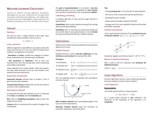
Optimization
Almost every machine learning method has an optimization
algorithm at its core.
Gradient Descent
Gradient Descent is used to find the coefficients of f that
minimizes a cost function (for example MSE, SSR).
Procedure:
à Initialization θ = 0 (coefficients to 0 or random)
à Calculate cost J(θ) = evaluate(f coefficients )
à Gradient of cost
7
789
J(θ) we know the uphill direction
à Update coeff θj = θj − α 7
J(θ) we go downhill
789
The cost updating process is repeated until convergence
(minimum found).
Batch Gradient Descend does summing/averaging of the
cost over all the observations.
Stochastic Gradient Descent apply the procedure of
parameter updating for each observation.
Tips:
- Change learning rate α (“size of jump” at each iteration)
- Plot Cost vs Time to assess learning rate performance
- Rescaling the input variables
- Reduce passes through training set with SGD
- Average over 10 or more updated to observe the learning
trend while using SGD
Ordinary Least Squares
OLS is used to find the estimator β that minimizes the sum
E
B
of squared residuals: (y ? − β @ − β 9 x ?9 ) F = y − X β
?CD
Using linear algebra such that we have β = (X G X) HD X G y
Maximum Likelihood Estimation
MLE is used to find the estimators that minimizes the
likelihood function:
L θ x = f 8 (x)
Linear Algorithms
9CD
density function of the data distribution
All linear Algorithms assume a linear relationship between
the input variables X and the output variable Y.
Linear Regression
Representation:
A LR model representation is a linear equation:
y = β @ + β D x D + ⋯ + β ? x ?
β @ is usually called intercept or bias coefficient. The
dimension of the hyperplane of the regression is its
complexity.

Learning:
Learning a LR means estimating the coefficients from the
training data. Common methods include Gradient Descent
or Ordinary Least Squares.
Variations:
There are extensions of LR training called regularization
methods, that aim to reduce the complexity of the model:
- Lasso Regression: where OLS is modified to minimize the
sum of the coefficients (L1 regularization)
E
?CD
B
(y ? − β @ − β 9 x ?9 ) F + λ |β 9 | = RSS + λ |β 9 |
9CD
- Ridge Regression: where OLS is modified to minimize the
squared sum of the coefficients (L2 regularization)
E
?CD
B
B
9CD
B
9CD
(y ? − β @ − β 9 x ?9 ) F F
F
+ λ β 9 = RSS + λ β 9
9CD
B
9CD
where λ ≥ 0 is a tuning parameter to be determined.
Data preparation:
- Transform data for linear relationship (ex: log transform
…for exponential relationship)
- Remove noise such as outliers
- Rescale inputs using standardization or normalization
Advantages:
+ Good regression baseline considering simplicity
+ Lasso/Ridge can be used to avoid overfitting
+ Lasso/Ridge permit feature selection in case of collinearity
Usecase examples:
- Product sales prediction according to prices or promotions
-.Call-center waiting-time prediction according to the
…number of complaints and the number of working agents
B
9CD
Logistic Regression
It is the go-to for binary classification.
Representation:
Logistic regression a linear method but predictions are
transformed using the logistic function (or sigmoid):
φ is S-shaped and map real-valued number in (0,1).
The representation is an equation with binary output:
y =
e Q RSQ T U T S⋯SQ V U V
1 + e Q RSQ T U T S⋯SQ V U V
Which actually models the probability of default class:
Learning:
p X =
eQ RSQ T U T S⋯SQ V U V
1 + e Q RSQ T U T S⋯SQ V U V
= p Y = 1 X
Learning the Logistic regression coefficients is done using
maximum-likelihood estimation, to predict values close to
1 for default class and close to 0 for the other class.
Data preparation:
- Probability transformation to binary for classification
- Remove noise such as outliers
Advantages:
+ Good classification baseline considering simplicity
+ Possibility to change cutoff for precision/recall tradeoff
+ Robust to noise/overfitting with L1/L2 regularization
+ Probability output can be used for ranking
Usecase examples:
- Customer scoring with probability of purchase
- Classification of loan defaults according to profile
Linear Discriminant Analysis
For multiclass classification, LDA is the preferred linear
technique.
Representation:
LDA representation consists of statistical properties
calculated for each class: means and the covariance matrix:
μ Z = D
E
x
E ?
[
?CD and σ F =
D
EH]
E
?CD
(x ? − μ Z )
LDA assumes Gaussian data and attributes of same σ 2 .
Predictions are made using Bayes Theorem:
P Y = k X = x =
P(k)×P(x|k)
]
cCD
P(l)×P(x|l)
to obtain a discriminate function (latent variable) for each
class k, estimating P(x|k) with a Gaussian distribution:
D Z x = x × μ Z
σ F − μ Z F
+ ln (P k )
2σF The class with largest discriminant value is the output
class.
Variations:
- Quadratic DA: Each class uses its own variance estimate
- Regularized DA: Regularization into the variance estimate
Data preparation:
- Review and modify univariate distributions to be Gaussian
- Standardize data to μ = 0, σ = 1 to have same variance
- Remove noise such as outliers
Advantages:
+ Can be used for dimensionality reduction by keeping the
…latent variables as new variables
F

Usecase example:
- Prediction of customer churn
Nonlinear Algorithms
All Nonlinear Algorithms are non-parametric and more
flexible. They are not sensible to outliers and do not require
any shape of distribution.
Classification and Regression Trees
Also referred as CART or Decision Trees, this algorithm is the
foundation of Random Forest and Boosted Trees.
Representation:
The model representation is a binary tree, where each
node is an input variable x with a split point and each leaf
contain an output variable y for prediction.
The model actually split the input space into (hyper)
rectangles, and predictions are made according to the area
observations fall into.
Learning:
Learning of a CART is done by a greedy approach called
recursive binary splitting of the input space:
At each step, the best predictor X 9 and the best cutpoint s
are selected such that X X 9 < s and X X 9 ≥ s
minimizes the cost.
- For regression the cost is the Sum of Squared Error:
E
?CD
(y ? − y)
- For classification the cost function is the Gini index:
F
E
G = p Z (1 − p Z )
?CD
The Gini index is an indication of how pure are the leaves,
if all observations are the same type G=0 (perfect purity),
while a 50-50 split for binary would be G=0.5 (worst purity).
The most common Stopping Criterion for splitting is a
minimum of training observations per node.
The simplest form of pruning is Reduced Error Pruning:
Starting at the leaves, each node is replaced with its most
popular class. If the prediction accuracy is not affected, then
the change is kept
Advantages:
+ Easy to interpret and no overfitting with pruning
+ Works for both regression and classification problems
+ Can take any type of variables without modifications, and
…do not require any data preparation
Usecase examples:
- Fraudulent transaction classification
- Predict human resource allocation in companies
Naive Bayes Classifier
Naive Bayes is a classification algorithm interested in
selecting the best hypothesis h given data d assuming there
is no interaction between features.
Representation:
The representation is the based on Bayes Theorem:
P h d = P(d|h)×P(h)
P(d)
with naïve hypothesis P h d = P x D h × …×P(x ? |h)
The prediction is the Maximum A posteriori Hypothesis:
MAP h = max P h d = max (P d h ×P h )
The denominator is not kept as it is only for normalization.
Learning:
Training is fast because only probabilities need to be
calculated:
P h = ?ErstEuvr w
uxyEs(U ∧ {)
and P x h =
tcc ?ErstEuvr ?ErstEuvr w
Variations:
Gaussian Naive Bayes can extend to numerical attributes
by assuming a Gaussian distribution.
Instead of P(x|h) are calculated with P(h) during learning:
μ x = D E
E
x ?
?CD and σ = D E
(x ? − μ x ) F
E ?CD
and MAP for prediction is calculated using Gaussian PDF
Data preparation:
f x μ x , σ =
1 2πσ eH(UH~) F€
- Change numerical inputs to categorical (binning) or near-
…Gaussian inputs (remove outliers, log & boxcox transform)
- Other distributions can be used instead of Gaussian
- Log-transform of the probabilities can avoid overflow
- Probabilities can be updated as data becomes available
Advantages:
+ Fast because of the calculations
+ If the naive assumptions works can converge quicker than
…other models. Can be used on smaller training data.
+ Good for few categories variables
Usecase examples:
- Article classification using binary word presence
- Email spam detection using a similar technique
K-Nearest Neighbors
If you are similar to your neighbors, you are one of them.
Representation:
KNN uses the entire training set, no training is required.
Predictions are made by searching the k similar instances,
according to a distance, and summarizing the output.

For regression the output can be the mean, while for
classification the output can be the most common class.
Various distances can be used, for example:
- Euclidean Distance, good for similar type of variables
d a, b =
E
?CD
(a ? − b ? ) F
- Manhattan Distance, good for different type of variables
E
d a, b = |a ? − b ? |
?CD
The best value of k must be found by testing, and the
algorithm is sensible to the Curse of dimensionality.
Data preparation:
- Rescale inputs using standardization or normalization
- Address missing data for distance calculations
- Dimensionality reduction or feature selection for COD
The prediction function is the signed distance of the new
input x to the separating hyperplane w:
f x =< w, x > + ρ = w G x + ρ with ρ the bias
Which gives for linear kernel, with x ? the support vectors:
Learning:
E
f x = a ? ×(x×x ? )) + ρ
?CD
The hyperplane learning is done by transforming the
problem using linear algebra, and minimizing:
Ensemble Algorithms
Ensemble methods use multiple, simpler algorithms
combined to obtain better performance.
Bagging and Random Forest
Random Forest is part of a bigger type of ensemble
methods called Bootstrap Aggregation or Bagging. Bagging
can reduce the variance of high-variance models.
It uses the Bootstrap statistical procedure: estimate a
quantity from a sample by creating many random
subsamples with replacement, and computing the mean of
each subsample.
Representation:
Advantages:
+ Effective if the training data is large
1
n
E
?CD
max 0,1 − y ? w. x † − b
+ λ||w|| F
For bagged decision trees, the steps would be:
- Create many subsamples of the training dataset
+ No learning phase
Variations:
- Train a CART model on each sample
+ Robust to noisy data, no need to filter outliers
Usecase examples:
- Recommending products based on similar customers
- Anomaly detection in customer behavior
Support Vector Machines
SVM is a go-to for high performance with little tuning
Representation:
In SVM, a hyperplane is selected to separate the points in
the input variable space by their class, with the largest
margin.
The closest datapoints (defining the margin) are called the
support vectors.
But real data cannot be perfectly separated, that is why a
C defines the amount of violation of the margin allowed.
The lower C, the more sensitive SVM is to training data.
SVM is implemented using various kernels, which define the
measure between new data and support vectors:
- Linear (dot-product): K x, x ? = (x×x ? )
- Polynomial: K x, x ? = 1 + (x×x ? )ˆ
- Radial: K x, x ? = e H‰ ((UHU V) )
Data preparation:
- SVM assumes numeric inputs, may require dummy
….transformation of categorical features
Advantages:
+ Allow nonlinear separation with nonlinear Kernels
+ Works good in high dimensional space
+ Robust to multicollinearity and overfitting
Usecase examples:
- Face detection from images
- Target Audience Classification from tweets
- Given a new dataset, calculate the average prediction
However, combining models works best if submodels are
weakly correlated at best.
Random Forest is a tweaked version of bagged decision
trees to reduce tree correlation.
Learning:
During learning, each sub-tree can only access a random
sample of features when selecting the split points. The size
of the feature sample at each split is a parameter m.
A good default is
p for classification and B for regression.
Š
The OOB estimate is the performance of each model on its
Out-Of-Bag (not selected) samples. It is a reliable estimate
of test error.
Bagged method can provide feature importance, by
calculating and averaging the error function drop for
individual variables (depending of samples where a
variable is selected or not).

Advantages:
In addition to the advantages of the CART algorithm
+ Robust to overfitting and missing variables
+ Can be parallelized for distributed computing
+ Performance as good as SVM but easier to interpret
Usecase examples:
- Predictive machine maintenance
- Optimizing line decision for credit cards
Boosting and AdaBoost
AdaBoost was the first successful boosting algorithm
developed for binary classification.
Representation:
A boost classifier is of the form
F G x =
G
sCD
f s (x)
where each f s is a week learner correcting the errors of the
previous one.
Adaboost is commonly used with decision trees with one
level (decision stumps).
Predictions are made using the weighted average of the
weak classifiers.
Learning:
The incorrectly predicted instance are given more weight.
Weak models are added sequentially using the training
weights, until no improvement can be made or the number
of rounds has been attained.
Data preparation:
- Outliers should be removed for AdaBoost
Advantages:
+ High performance with no tuning (only number of rounds)
Interesting Resources
Machine Learning Mastery website
> https://machinelearningmastery.com/
Scikit-learn website, for python implementation
> http://scikit-learn.org/
W.Chen probability cheatsheet
> https://github.com/wzchen/probability_cheatsheet
HackingNote, for interesting, condensed insights
> https://www.hackingnote.com/
Seattle Data Guy blog, for business oriented articles
> https://www.theseattledataguy.com/
Explained visually, making hard ideas intuitive
> http://setosa.io/ev/
This Machine Learning Cheatsheet
> https://github.com/remicnrd/ml_cheatsheet
Each training set instance is initially weighted w x ?
= D E
One decision stump is prepared using the weighted
samples, and a misclassification rate is calculated:
ε =
E
?CD
(w ? ×p v x ? )
E
w
Which is the weighted sum of the misclassification rates,
where w is the training instance i weight and p v x ? its
prediction error (1 or 0).
?CD
A stage value is computed from the misclassification rate:
stage = ln ( 1 − ε )
ε
This stage value is used to update the instances weights:
rst v×
w = w×e