Physics 111 ~ BSC Student Evaluation of Lab Write-Up

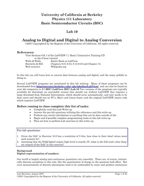
University of California at Berkeley 

Physics 111 Laboratory 

Basic Semiconductor Circuits (BSC) 

Lab 10 

Analog to Digital and Digital to Analog Conversion 

©2007 Copyrighted by the Regents of the University of California. All rights reserved. 

References: 

View Sections 6 & 7 of the LabVIEW 7.1 Basic I Interactive Training CD 

or the 6 hour tutorial 

Wells & Wells Entire Book on LabView. 

Horowitz & Hill Chapters 8.01-8.04, 9.15-9.23 and Chapter 15. 

Web resource Wikipedia.org 

In this lab you will learn how to convert data between analog and digital, and the many pitfalls in 

doing so. 

Several LabVIEW programs are mentioned in this lab writeup. Many of these programs can be 

downloaded from http://socrates.berkeley.edu/~phylabs/bsc/LabView/ and can also be found on 

your lab computers in C:\BSC\LabView BSC\Lab-10 Two versions of the programs are typically 

available for download: an executable version that should run without LabVIEW (but requires a 

large download from National Instruments, which should occur automatically, and only needs to be 

done once) and should run on PC’s, Mac’s and Linux boxes; and the original LabVIEW source code 

which requires LabVIEW. 

Before coming to class complete this list of tasks: 

• Completely read this Lab Write-up 

• Answer the pre-lab questions utilizing the references and this write-up 

• Perform any circuit calculations or anything that can be done outside of lab. 

• Begin and if possible complete programming tasks in this lab write-up 

• Plan out how to perform Lab exercises in this write-up. 

Pre-lab questions: 

1. Given the DAC in Exercise 10.2 has a resolution of 5 bits, how close to their ideal values must 

each resistor be? 

2. Assuming that the DAQ digital output high level is exactly 5V, what is the full scale value (largest 

output) of the DAC in this exercise? 

Background 

Digital representation of numbers 

Our world is largely analog and continuous; quantities vary smoothly. There are, of course, intrinsically 

discrete exceptions to this rule, like the quantization of charge or the quantum hall effect. But 

even measurements of discrete phenomena tend to be confounded by noise and produce continuous 

Last Revision: August 2007 Page 1 of 22 

©2007 Copyrighted by the Regents of the University of California. All rights reserved.

Physics 111 BSC Laboratory Lab 10 LabVIEW Programming 

data. Internally, however, modern computers 1 deal only with discrete quantities; specifically, they 

deal only with quantities take on only two values: on or off. This so-called digital representation of 

information has many advantages over analog representations, most importantly that digital information 

is relatively immune to noise. If a 0, or off state, is represented by a voltage near 0, and a 1, 

or on state is represented by a voltage near 4 (a scheme used by a common family of digital devices 

called TTL logic), then noise is unlikely to cause a fluctuation great enough to confuse the two. 

Because computers can only represent two states, numbers are stored in binary, or base 2. The digits 

in a base 2 number are called bits, thus, a typical number in base 2 number is a collection of bits 

like 01011010. Numbers are decoded using a power series in 2: 

∞ 

∑ 

n= 

0 

n 

a 2 = a 2 + a 2 + a 2 + a 2 + L 

n 

0 1 2 3 

0 1 2 3 

where the an 

are the series of bits used to represent the number. Thus, 

Base 

10 

0 1 2 3 4 5 6 7 

Base 2 00 00 01 01 10 10 11 11 

0 1 0 1 0 1 0 1 

The more bits used, the larger the integer number that can be represented. Non-integer numbers are 

represented by multiplying in an appended exponent; thus, the more bits, the greater the precision 

of the number. 

Eight bits taken together constitute a byte, and computers are typically organized around byte processing, 

not bit processing. 

Conversion 

Since the real world is analog, but the computer world is binary, we need to be able to convert signals 

between the two. Devices that change an analog signal to a digital signal are called analog to 

digital converters (ADC). Devices that change a signal the other way, from digital to analog, are 

called digital to analog converters (DAC). Both are important; DACs are used to control experiments, 

while ADCs are used to read data from experiments. 

1 Originally, computers were analog, and did computations in ways similar to the way that you did 

computations in your RMS converters. Programming was done by wiring patch panels, as can be 

seen in the photos of the analog computers below. 




Sampling 

Real-world signals are continuous in time as well as level. Thus, to represent a time-varying signal, 

we build up a table of the value of the signal as a function of time, for example: 

Time Signal 

0 1.000 

0.125 0.649 

0.250 -0.156 

0.375 -0.853 

0.500 -0.951 

0.625 -0.383 

0.750 0.454 

0.875 0.972 

1.000 0.809 

1.125 0.078 

1.250 -0.707 

1.375 -0.997 

1.500 -0.588 

1.625 0.233 

1.750 0.891 

1.875 0.924 

2.000 0.309 

These values are called samples. 




We can better visualize sample tables with a graph. The curve in upper plot of the graph below 

represents a signal to be sampled. The dots are the samples. If we then use the samples to represent 

the signal, we get the signal in the lower plot, where the points are joined by the dashed line. 

Sampling always approximates the signal. How accurate is the representation? There are two basic 

limits on the accuracy, resolution and sampling rate. 

Resolution 

The number of bits available to represent each sample is called the resolution. In base 2, the number 

of levels that can be represented by an n bit sample is 2 n . Thus, for 8 bits (the number of bits in 

a typical low end converter) there are 256 levels, while for 24 bits (the maximum common 2 converter 

resolution) there are 16,777,216 levels. 

It is rare that we would need precisions better than 1 part in 1000, or 10 bits. What then is the 

point of going to higher resolution? Higher resolution provides greater range. It is uncommon for 

the signal amplitude to exactly match the full-scale value of the converter. Typically, we might have 

a margin of over a factor of ten; perhaps 4 bits. Thus, to get 10 bit accuracy we would need a 14 bit 

converter. 

Even if the maximum amplitude of our signal matches the full-scale value of the converter, the signal 

amplitude is likely to vary significantly over time. (This is called “dynamic range.”) For instance, 

the sound level from a symphony orchestra varies from about 40dB to 130dB. (Sounds at 

130dB are rare; the “cannon” in the Tchaikovsky’s 1812 overture are one example.) Consequently, 

the amplitude of the sound waves varies by a factor of about 30,000. This seemingly requires about 

15 bits. But with 15 bits, the lowest levels would be represented by just one bit level changes. A 

sine waves represented by only one bit becomes a square wave. We would prefer to better represent 

low signals; perhaps six bits for the lowest levels. Thus, we would need a 21 bit converter to well 

represent the signal. 3 However, CDs use only 16 bits. 4 To record symphonic music without distortion, 

engineers typically compress the signal; the quietest passages are made louder, while the loudest 

passages are softened. 

2 The National Instruments PXI-4461, available for a mere $3995. 

3 In principle, using floating point numbers (a mantissa and an exponent) would better represent the 

music. But floating point converters are difficult to make and very rare. After the signal is sampled, 

however, can convert the numbers to floating point without much loss of information. This is one of 

the tricks used in compressing music in schemes like mp3s. 

4 The program Wave_Quantization illustrates the effects of resolution on an audible signal. 




A higher resolution also makes it easier to extract signals from noise. Say we are using a 10 bit 

ADC to digitize a small signal which is masked by noise whose level is 10 bits. We could not amplify 

the signal because the noise would cause our converter to saturate. You might think that the signal 

would have to be larger than one bit to be detected. Curiously, if there were no noise, this would be 

true. But with noise, we can detect signals which are smaller than one bit. 

DC. 

5 Still, its much better 

not to have to rely on the noise to make the signal measurable, and we would be better off with a 

higher precision A 

Sampling Rate 

The effects of the sampling too slowly are more subtle than the effects of limited resolution. When 

we sample too slowly, we do not get an adequate representation of the signal; in fact, we may be 

badly confused by spurious signals. These effects were codified by Nyquist, who determined that: 

A signal can only be perfectly represented by a samples taken at more than twice 

the maximum frequency in the signal. 

Thus if we sample at ratef s , then the signal must contain no information with frequencies higher 

than f s 2 . This latter frequency is called the Nyquist Frequency. 

If we violate Nyquist’s theorem we get aliasing; signals at higher frequencies get shifted down to 

lower frequencies. For example, if we have a sinusoidal signal with frequency 1Hz, and sample it at 

frequency 10.4Hz, we get a good representation of the signal (but note that the peaks are still 

slightly distorted☺ 

But if we sample the signal below the minimum sample frequency for this wave of 2 Hz, we get an 

aliased signal. For instance, if we sample the signal at a frequency of 1.7 Hz we get: 

5 The technique of deliberately adding noise to a signal to reduce the effects of quantization is called 

dithering: see http://en.wikipedia.org/wiki/Dither 




In this case, we get a garbage signal, and we might well guess that the signal has been aliased. But 

sometimes we get seemingly good signals, as in this case where we sample at a frequency of 0.53Hz: 

It is very easy to confuse a signal like this one for a real signal. We need to be very careful when 

interpreting a sampled signal. 

While aliased signals can look quite confused, it is quite easy to understand the origin of aliasing in 

frequency space. Signals above the Nyquist frequency do not simply vanish; they get mirrored 6 into 

frequencies below the Nyquist frequency. Thus, if we sample a signal that has desired frequency 

content below the Nyquist frequency (shown in green in the diagram below) and undesired “noise” 

about the Nyquist frequency (shown in pink), the undesired signal will be reflected around the Nyquist 

Frequency into the midst of the desired signal. 

6 The program Whistle_Aliasing audibly demonstrates mirroring, including the effects of multiple 

mirroring. 




The location of the mirrored, or aliased, signals is easy to predict: 

( f 

st 

) 

f = f − − f 

Observed Nyquist Actual Nyqui 

= f − f 

Sample Actual 

Actually, this is only the first of the mirrored frequencies. Signals are mirrored again and again 6 

like in a barbershop mirror. But each time they get mirrored, their amplitude decreases, so we typically 

ignore all but the first mirror. 

Picking a Sample Frequency 

It is always safest and easiest to pick 7 a sampling frequency well above the highest anticipated frequency. 

A factor of ten to hundred times higher provides a comfortable margin. But there are times 

when it is not feasible to pick such a high frequency. Your converter may be incapable of sampling 

fast enough, or the desired rate may be technologically infeasible. Even if a converter with the desired 

sample rate exists, it may be prohibitively expensive; the cost of ADCs and DACs increase rapidly 

with sampling speed. For instance a 250kS/s (kilo Sample/sec) ADC costs just $375 today 

(2005): a 10MS/s card costs $4000, and a 1GS/s card costs $10,000. And then, even if you do have an 

appropriately fast card, you may find that the fast data rate overwhelms your system, and you may 

be forced to sample slower anyway. 

Nyquist’s theorem states that you need only sample at twice the desired frequency. What happens if 

you are close to the Nyquist limit? The sampled signal may not appear to resemble the actual signal. 

For instance, if you sample a sine wave at 2.35 times its frequency, you get: 

Sampling at 2.05 times the frequency yields: 

7 The program Wav_Aliasing audibly demonstrates the effects of aliasing on a music sample. 




Neither sampled signal resembles the original signal. Is Nyquist wrong? Comparing the spectrum 

of the original signal to the sampled signal illuminates the problem: 

The original signal contains one clean peak that the original frequency. The sampled signal has an 

extra peak at a frequency a bit higher than the original. 8 The amplitude modulations in the sampled 

signal are due to these two peaks in the sampled spectrum beating against each other. We can 

largely recover the original frequency by low-pass filtering the sampled signal to destroy the spurious 

peak: 

Unfortunately, filtering is not always easy to accomplish. It is relatively easy to filter a signal on a 

computer by taking its Fourier transform and discarding the spectral content about the Nyquist frequency. 

But filtering with real-world components in real time is not nearly so easy. A simple one 

pole RC filter does not roll off fast enough, so we need to cascade filters to make them roll off faster: 

8 More precisely, signals mirror up as well as down around the Nyquist frequency, so the frequency 

of the second peak is at 1.05. 




The 6 th order RC filter depicted above rolls off quite fast; its transfer function is down by two orders 

of magnitude one octave about its design corner at 1Hz. But it has also significantly reduced the 

signal amplitude in the passband below 1. Signal aliasing may not be a problem, but the original 

signal will be distorted. 

Filter design is an exceedingly complicated topic, and there are better filters exist than simple RC 

designs. Typical advanced designs are called Butterworth, Chebyshev, and Bessel filters, and their 

response is plotted below. 

The order of the filters have been adjusted so that they attenuate by a factor of 100 one octave about 

their design frequency of 1Hz. The Butterworth and Chebyshev filters look very attractive; they cut 

off quickly, but leave the pass-band relatively unmodified. Unfortunately, their transient response 

is poor. Feed a step into them, and the will distort the signal: 

All the filters delay the onset of the step, and The Butterworth and Chebyshev filters ring significantly. 

The Bessel filters has the best step response, but its frequency response is not as good as the 

Butterworth and Chebyshev filters. In sum, perfect filters cannot be constructed outside of a computer. 

Even in a computer, it is difficult to make a perfect filter. The spectrum of the signal sampled 

at 2.05 contains one major spurious peak above the Nyquist frequency, but is also contains 

smaller spurious peaks below the Nyquist frequency. These peaks distort the signal. For instance, 

if we sample a signal consisting of two equal amplitude sine waves at frequencies of 0.7 and 1, at a 

sampling frequency of 3, we can do a fair job of reconstructing the original signal: 




Nonetheless, the spectrum shows many spurious peaks, 

whose effects are visible on careful comparison 

with the original signal. With the ideal, computer 

filter, however, the spectrum is much closer to 

the original signal spectrum and differences to the original signal are insignificant. The effects of 

imperfect filtering are even more visible for an AM modulated carrier wave: 

One should remember that the sampled signal is just a table of values. When we plot the sampled 

data, 

we need to interpolate between the sampled points. 

There are several ways to interpolate. 

Starting from uninterpolated data: 




we 

can step interpolate (used on most DACs), ramp interpolate (used on some expensive DAQs) or 

comb 

interpolate. 

Comb interpolation, which uses a sequence of infinite delta functions, each with area equal to the 

amplitude of sample at successive points, is difficult to use in the real world, because delta functions 

are unphysical. Surprisingly though, it is theoretically optimal, 

as can be seen from the proof of Ny- 

quist’s theorem, http://en.wikipedia.org/wiki/Nyquist_theorem 

Digital to Analog Converters 

There are several ways to build digital to analog converters, but the simplest way is with a scaled 

resistor 

network: 

bn 

This is just an opamp adder circuit, in which each bits bn 

is added in with weight 2 . In practice it 

is difficult to make a high resolution DAC with a scaled resistor network because it requires pre- 

cisely scaled resistors over a very wide range. It is much easier to make precise resistors over a narrow 

range; 9 a common DAC that takes advantage of this fact uses a ladder network: 

9 Precision resistors can be fabricated over a narrow range by a technique called laser trimming, in 

which a laser is used to etch away small sections of the resistive material while monitoring the total 

resistance. Laser trimmed resistors made on the same chip are particularly precise, and will also 

track together as the temperature changes. 







Like the scaled resistor ADC, this circuit also adds together appropriately weighted bits. 

Practical Filtering and Aliasing Advice 

ADCs: Always make sure that you are not being fooled by aliasing artifacts. The best way 

to test for the presence of artifacts is to look at the signal with your entire detector, amplifier, 

and ADC chain in place and adjusted to your contemplated settings, but with your experiment 

turned off so that you are receiving no real data. If you observe a significant signal, 

you then know that you are observing an artifact. 

• Occasionally, the received signal is so free of noise that aliasing of unwanted 

frequencies is unimportant. If so, either: (1) sample at twenty or more times the desired 

signal frequency, or (2) sample closer to twice the desired signal frequency and 

use digital filtering to remove the artifacts. 

• The maximum frequency of most received signals is naturally limited by the 

detector that produced the signal, or by the detector amplifiers. If possible, sample 

at a frequency that is higher than twice the maximum frequency of the received signal, 

using digital filtering, as necessary, to remove the artifacts. 

• If the desired signal is centered around a narrow band of frequencies, you 

may be able to ignore aliasing artifacts. Set your ADC to sample at several times 

the band center frequency. Establish that you can ignore aliasing artifacts by the 

test described above, concentrating only on signals in the band of interest. If you do 

observe artifacts, you may be able to get rid of them by changing your sample frequency 

so that the spurious signals alias to a different frequency that is out of your 

band of interest. 

• In necessary, employ a filter to remove the high frequency noise. Some ADCs 

come with anti-aliasing filters built-in. These are filters are likely to be quite good; 

use them before building your own. Otherwise, use your own anti-aliasing filter. If 

you can, use a simple RC low-pass filter designed to cut off at a much higher than 

your signal frequency, (so that the pass-band attenuation at the signal frequency is 

small) and sample at a frequency much higher than the filter’s cut off frequency (so 

that the filter attenuation is large above the Nyquist frequency.) If you cannot 

space your cutoff and sample frequency so generously, obtain a commercial filter, or, 

if all else fails, build a sophisticated multipole filter optimized for your application. 

DACs: 

• If your DAC and memory can support it, use a sample frequency 20 to 200 

times greater than your signal frequency. 

• The device you are driving may not care about spurious high frequency components. 

In this case, you can run quite close to the Nyquist frequency without filtering. 

• If your signal is close to the Nyquist frequency, use a filter. Some DAC’s 

come with high quality filters; use them if available. Otherwise, use a commercial 

filter, or a simple RC filter. If you signal is close to a pure sine wave, and you can 

tolerate variations in its amplitude with frequency, you may be able to generate 

relatively undistorted signals quite close to the Nyquist frequency. 

• If nothing else works, design a higher order filter optimized for your signal. 




Analog to Digital Converters 

The simplest way to make an n-bit ADC is to have 2 separate comparators, each comparing the 

input voltage to one of the set of all the voltage levels allowed by the resolution of the ADC: 

n 

An encoder determines the highest “on” comparator, and encodes this information into a number. 

Such flash, or parallel recorders are very fast, and are used in high frequency applications. But they 

are not feasible for high resolution ADCs, as every voltage level requires a separate comparator. 

Conversion is more commonly done by a successive approximation ADC. This type of ADC successively 

refines a guessed value in a loop. The steps in the loop are: 

1. Convert the guess to a voltage using a DAC. 

2. Compare this guess voltage to the input voltage. 

3. Refine the guess: 

a. If the guess is too low, make a new guess that is higher. The new guess should be 

half way between the current guess and the last known guess that was too high. 

b. If the guess is too high, make a new guess that is lower. The new guess should be 

half way between the current guess and the last known guess that was too low. 

4. Begin the cycle again if the conversion has not exhausted all the DAC bits. Otherwise, call 

the final guess the answer and end the loop. 

The loop is initialized by setting the last know limits to be the minimum and maximum values accepted 

by the ADC, and setting the first guess to be half way in between. This process is best illustrated 

by a tree diagram, shown here for an ADC whose range is 0 to 16V: 




4.0 

12.0 

2.0 

5.0 

7. 7.00 

9. 9.00 

11.0 

13. 13.00 

15.0 

0.5 

1.5 

2.5 

3.5 

4.5 

5.5 

6.5 

7.5 

8.5 

9.5 

10.5 

11.5 

12.5 

13.5 

14.5 

15.5


In the lab 

(A) Aliasing and Sample Rate 

10.1 Run the program Sampling_Simulator. With filtering set to No Filter, explore the effects of 

the sample rate on Pure Sine and Square waves. Use both Flat Interpolation and Linear Interpolation. 

In your lab notebook, record your answers to the following questions: 

1. Sample a 1Hz, phase 90 Sine wave at 4Hz. Do you get a reasonable facsimile of the original 

sine wave? Now change the phase. What happens? Do you still get a reasonable facsimile? 

Restore the phase to 90. What happens when you change the sample rate to 4.01? 

Can you account for the difference? 

2. Repeat these measurements with a Square wave, and record your answers. 

3. Using a 1Hz Sine wave, try some inadequate sampling rates, say 1.9, 1, 0.9, 0.5 and 

0.47Hz. Can you account for the features you observe? 

4. Explore the effects of inadequate sampling rages on a Square wave. 

5. What sample rate is necessary to give a reasonable facsimile of a sine wave, and what sample 

rate gives a reasonable facsimile of a square wave? Why are these frequencies different? 

6. Now find appropriate sample rates for the Two Tone, AM, and FM signals. Ironically, you 

may conclude that these signals can be sampled at a lower rate than the pure sine wave. 

This is probably because these signals are so complex that the sampling artifacts so clearly 

visible with the Sine signal are masked. 

7. Now try the Realistic Low Pass Filter with the Sine signal and various sample rates. 

Can you employ lower sample rates? Look at the amplitude as well as the form of the sampled 

and filtered signals. Is the amplitude sometimes incorrect even when the form is correct? 

8. Look at Square waves with the Realistic Low Pass Filter. What is the effect of the sample 

rate? Using the Expanded Time Axis, cycle between Realistic Low Pass Filter and 

No Filter. Note that the filter causes the rise and falls to be delayed. What is the size of 

the delay? Does it depend on the sample rate? Note that the realistic filter is a 3 rd order 

Butterworth. Does this fact explain the delay? 

9. Look at the Two Tone, AM, and FM signals. Does the filter help? 

10. Now go back to a 1Hz Sine wave, and set the sample rate to just above 2Hz, say 2.1Hz. 

Does any interpolation method produce a reasonable facsimile of the wave with the Realistic 

Low Pass Filter? (Hint: Ask what is reasonable?) Switch to the Ideal Low Pass Filter. 

Is it better? What do your signals look like for the different interpolations? Which one 

gets the amplitude correct? With Comb Interpolation, how low a sample frequency can 

you use? Try sample rates of 2.02 and 2.01Hz. In principle, you should be able to go down 

to 2.00Hz, but, in practice, 2.01Hz has problems. Can you explain why? (This is hard and 

is not obvious from the material covered in this writeup or in lecture.) 

11. Now go to a sample rate of 1.95Hz. Is the Ideal Low Pass Filter any better than the Realistic 

Low Pass Filter? 

12. With the Ideal Low Pass Filter and Comb Interpolation, explore sampling ranges 

above 2.00Hz for the Two Tone, AM, and FM signals. How good are the sampled signals? 

Try a Square Wave? Why is the sampled signal no good? 

� Show and discuss your results to the TA’s. 

10.1.1 Learn to program in LabVIEW 7.1 by doing the exercises in sections 6-7 in National Instrument’s 

Basic 1 Interactive Training. The Files can be downloaded from 

http://socrates.berkeley.edu/~phylabs/bsc/LabView While you may work with your partner, 

both of you will be expected to learn to program in LabVIEW separately. 

� Demonstrate the programs created in the Exercises on the CD to the TA’s. and discuss 

any confusing parts of the the tutorial. 




(B) Digital to Analog Conversion 

10.2 Build a scaled resistor DAC: 

Use the digital outputs 10 of your DAQ card to drive the outputs; in particular, use the low order bits 

marked P0.0 (lowest) to P0.4. These digital outputs switch between approximately 0 and +5V; consequently 

your converter will output negative voltages. You will have to scale your resistors up from 

the values used in the above schematic; determine the base value (the “1”) from the requirement 

that the current drawn from any of the digital outputs individually should be less than 2.5ma. We 

do not have the precise resistor values that you will need. You will have to synthesize the correct 

values by combining two or more resistors. 

Correct your Pre-Lab Question calculation of the full scale voltage of the DAQ by measuring the actual 

high level output of the DAQ. 11 Build a LabVIEW driver for your DAC. 12 Your driver’s front 

panel should look something like: 

where the Bit Pattern indicator is included for debugging purposes. You will have to scale the output 

voltage to a bit pattern. You should make sure that you cannot drive your DAC with an out-ofrange 

bit pattern. A convenient way to assure that you don’t is to use LabVIEW’s In Range and Co- 

erce operator, which can be found amongst the comparison operators menu. Use your scope or 

10 The digital lines are available on your interface box as screw terminals. Strip about ¼ inch of insulation 

from a wire, push it into the rectangular hole, and gently tighten the screw below. Do not 

overtighten, and make sure that you use the correct screw driver. 

11 You may find it helpful during this exercise to drive the digital lines with the DAQ’s debugging 

interface. Open the DAQ Assistant for the DAQ, configure it for digital output, and go to the Test 

tab. 

12 The program DAC.vi implements this functionality, and you may use it to get started. You will 

not be able to access its block diagram. 




multimeter to test your DAC. Note that even though you are driving the digital lines with one byte 

(actually only 5 bits in one byte) of data, the DAQ Assistant expects an array. Use the Build Array 

operator to turn your byte into a one element array of bytes. 

10.3 Write a program to test your DAC. 13 The program’s front panel should look something like 

The program should: 

1. Loop through all of the possible DAC output levels. 

2. At each level 

a. Display the Desired DAC output with an indicator. 

b. Drive the DAC 

c. Wait twenty milliseconds for the DAC to settle. Use the Wait operator 

found under Time and Dialog Operators menu. 

d. Read the output of the DAC with one of the analog input channels of the DAQ. 

Hint: Use a Stacked Sequence Structure for steps b-d 

e. Output the DAC voltage. 

i. Display the DAC output with an indicator. 

ii. Store the current Desired Output and Actual Output in an array and use 

an XY plot to display a graph of the Desired Output vs. the Actual Output. 

The best way to do this is with shift registers. The program Running 

XY Graph Example demonstrates the technique. 

13 The program Test_DAC.vi implements this functionality, and you may use it to get started. You 

will not be able to access its block diagram. 




Hint: Also use Build Arrays and the Bundle functions. If your having trouble, 

be sure to review the array section of the Training Video. 

iii. Subtract the Desired Output from the Actual Output to find the DAC Deviation, 

and display a running graph. 

� Explain the systematic features in the DAC Deviation graph. What is the maximum error? 

Demonstrate your program and the DAC Driver subvi to the TA’s, and explain their block diagrams. 

(C) Analog to Digital Conversion 

10.4 Build a successive approximation ADC by adding a comparator to your DAC: 

Write the following programs to complete the ADC implementation: 

1. Compare Trial.vi. This subroutine should accept a Trial Voltage, write it to the 

DAC, wait 10ms for the DAC to settle, measure the output voltage of the comparator, 

and compare this voltage to some fixed voltage to determine if the Trial Voltage is 

greater than or less than the ADC Input Voltage. The front panel of the vi should 

look something like: 

Hint: Again, The Stacked Sequence Structure works well for timing control. 

2. ADC.vi. This routine should guess successive Trial Voltage’s until the ADC converges. 

You may find it helpful to organize your iterations in a for loop, remembering 

the previous high and low guesses from iteration to iteration with shift registers, 

Also Case Structures and Expression Nodes are helpful. For debugging purposes, 

you might wish to put in an indicator giving the current guess, and a switch controlling 

a 1s per iteration delay. Your front panel should look something like: 

To help you get started, working versions of these programs are available on the lab computers. The 

block diagrams of these programs are inaccessible. You may also use the program Set Voltage to be 

Converted to set precise voltages on the DAQ analog output channel AO-0. 

10.5 Write a program to test the ADC. The program should be similar to your DAC tester except 

that it should convert an essentially continuous voltage ramp. The front panel of the program 

should look something like: 




� Explain the systematic features in the ADC Deviation graph. What is the maximum error? 

Demonstrate your program and its subvis to the TA’s, and explain their block diagrams. 

10.6 The routine Test DAQ ADC and DAC.vi is very similar to the Test ADC routine that you just 

wrote, but tests the DAC and ADC on the DAQ. After attaching the A0 0 output to the AI 7 input, 

run the routine to test the accuracy of the DAQ converters. The DAQ DAC and ADC are both 12 bit 

converters. How big is a 1bit error? Are any of the errors larger than one bit? Which converter do 

you think you are testing: the DAC or the ADC? 

(D) Filtering 

10.7 Use the program Sine_DAQ_Drive.vi to output a 5V sine wave on AO-0. The sample rate is 

10kHz. The drive frequency is adjustable; look at the output on a scope for a range of frequencies. 

(Don’t exceed the Nyquist frequency.) About when is the signal acceptable? Now use 3.3k resistors 

to construct simple low pass filters with cut off frequencies near 10kHz and 1kHz. Drive the filters 

with the output from the DAQ. Draw pictures of the waveforms, and determine when the signal is 

acceptable. Note both amplitude changes and phase delays. 




Physics 111 ~ BSC Student Evaluation of Lab Write-Up 

Now that you have completed this lab, we would appreciate your comments. Please take a few moments to 

answer the questions below, and feel free to add any other comments. Since you have just finished the lab it 

is your critique that will be the most helpful. Your thoughts and suggestions will help to change the lab and 

improve the experiments. 

Please be specific, use references, include corrections when possible, using both sides of the 

paper as needed, and turn this in with your lab report. Thank you! 

Lab Number: Lab Title: Date: 

Which text(s) did you use? 

How was the write-up for this lab? How could it be improved? 

How easily did you get started with the lab? What sources of information were most/least helpful in getting 

started? Did the pre-lab questions help? Did you need to go outside the course materials for assistance? 

What additional materials could you have used? 

What did you like and/or dislike about this lab? 

What advice would you give to a friend just starting this lab? 

The course materials are available over the Internet. Do you (a) have access to them and (b) prefer to use 

them this way? What additional materials would you like to see on the web?

Physics 111 ~ BSC Student Evaluation of Lab Write-Up

You also want an ePaper? Increase the reach of your titles

Delete template?

Save as template?