Introduction to Time Series Analysis. Lecture 11. Peter Bartlett

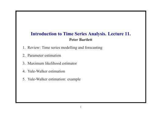
Introduction to Time Series Analysis. Lecture 11.
Peter Bartlett
1. Review: Time series modelling and forecasting
2. Parameter estimation
3. Maximum likelihood estimator
4. Yule-Walker estimation
5. Yule-Walker estimation: example
1

Review (Lecture 1): Time series modelling and forecasting
1. Plot the time series.
Look for trends, seasonal components, step changes, outliers.
2. Transform data so that residuals are stationary.
(a) Remove trend and seasonal components.
(b) Differencing.
(c) Nonlinear transformations (log, √ ·).
3. Fit model to residuals.
4. Forecast time series by forecasting residuals and inverting any
transformations.
2

Review: Time series modelling and forecasting
Stationary time series models: ARMA(p,q).
•p = 0: MA(q),
•q = 0: AR(p).
We have seen that any causal, invertible linear process has:
an MA(∞) representation (from causality), and
an AR(∞) representation (from invertibility).
Real data cannot be exactly modelled using a finite number of parameters.
We choose p,q to give a simple but accurate model.
3

Review: Time series modelling and forecasting
How do we use data to decide on p,q?
1. Use sample ACF/PACF to make preliminary choices of model order.
2. Estimate parameters for each of these choices.
3. Compare predictive accuracy/complexity of each (using, e.g., AIC).
NB: We need to compute parameter estimates for several different model
orders.
Thus, recursive algorithms for parameter estimation are important.
We’ll see that some of these are identical to the recursive algorithms for
forecasting.
4

Review: Time series modelling and forecasting
Model: ACF: PACF:
AR(p) decays zero forh > p
MA(q) zero forh > q decays
ARMA(p,q) decays decays
5

Introduction to Time Series Analysis. Lecture 11.
1. Review: Time series modelling and forecasting
2. Parameter estimation
3. Maximum likelihood estimator
4. Yule-Walker estimation
5. Yule-Walker estimation: example
6

Parameter estimation
We want to estimate the parameters of an ARMA(p,q) model.
We will assume (for now) that:
1. The model order (p and q) is known, and
2. The data has zero mean.
If (2) is not a reasonable assumption, we can subtract the sample mean ¯y,
fit a zero-mean ARMA model,
φ(B)Xt = θ(B)Wt,
to the mean-corrected time series Xt = Yt − ¯y,
and then use Xt + ¯y as the model for Yt.
7

Parameter estimation: Maximum likelihood estimator
One approach:
Assume that {Xt} is Gaussian, that is,φ(B)Xt = θ(B)Wt, where Wt is
i.i.d. Gaussian.
Chooseφi,θj to maximize the likelihood:
L(φ,θ,σ 2 ) = f φ,θ,σ 2(X1,...,Xn),
where fφ,θ,σ2 is the joint (Gaussian) density for the given ARMA model.
(c.f. choosing the parameters that maximize the probability of the data.)
8

Maximum likelihood estimation
Suppose that X1,X2,...,Xn is drawn from a zero mean Gaussian
ARMA(p,q) process. The likelihood of parameters φ ∈ R p ,θ ∈ R q ,
σ 2 w ∈ R+ is defined as the density of X = (X1,X2,...,Xn) ′ under the
Gaussian model with those parameters:
L(φ,θ,σ 2 w) =
1
(2π) n/2 exp
1/2
|Γn|
�
− 1
2 X′ Γ −1
�
n X ,
where |A| denotes the determinant of a matrix A, and Γn is the
variance/covariance matrix of X with the given parameter values.
The maximum likelihood estimator (MLE) ofφ,θ,σ 2 w maximizes this
quantity.
9

Parameter estimation: Maximum likelihood estimator
Advantages of MLE:
Efficient (low variance estimates).
Often the Gaussian assumption is reasonable.
Even if{Xt} is not Gaussian, the asymptotic distribution of the estimates
( ˆ φ, ˆ θ,ˆσ 2 ) is the same as the Gaussian case.
Disadvantages of MLE:
Difficult optimization problem.
Need to choose a good starting point (often use other estimators for this).
10

Preliminary parameter estimates
Yule-Walker for AR(p): Regress Xt ontoXt−1,...,Xt−p.
Durbin-Levinson algorithm withγ replaced by ˆγ.
Yule-Walker for ARMA(p,q): Method of moments. Not efficient.
Innovations algorithm for MA(q): withγ replaced by ˆγ.
Hannan-Rissanen algorithm for ARMA(p,q):
1. Estimate high-order AR.
2. Use to estimate (unobserved) noiseWt.
3. Regress Xt ontoXt−1,...,Xt−p, ˆ Wt−1,..., ˆ Wt−q.
4. Regress again with improved estimates ofWt.
11

Yule-Walker estimation
For a causal AR(p) model φ(B)Xt = Wt, we have
⎛ ⎛ ⎞⎞
E
p�
⎝Xt − ⎠⎠
= E(Xt−iWt) for i = 0,...,p
⎝Xt−i
j=1
φjXt−j
⇔ γ(0)−φ ′ γp = σ 2
γp −Γpφ = 0,
and
where φ = (φ1,...,φp) ′ , and we’ve used the causal representation
Xt = Wt +
to calculate the values E(Xt−iWt).
12
∞�
j=1
ψjWt−j

Yule-Walker estimation
Method of moments: We choose parameters for which the moments are
equal to the empirical moments.
In this case, we choose φ so that γ = ˆγ.
Yule-Walker equations for ˆ φ:
These are the forecasting equations.
We can use the Durbin-Levinson algorithm.
13
⎧
⎨ˆΓp
ˆ φ = ˆγp,
⎩
ˆσ 2 = ˆγ(0)− ˆ φ ′ ˆγp.

Some facts about Yule-Walker estimation
• If ˆγ(0) > 0, then ˆΓm is nonsingular.
• In that case, ˆ φ = ˆ Γ −1
p ˆγp defines the causal model
Xt − ˆ φ1Xt−1 −···− ˆ φpXt−p = Wt, {Wt} ∼ WN(0,ˆσ 2 ).
• If {Xt} is an AR(p) process,
�
ˆφ ∼ AN φ, σ2
n Γ−1
�
p
�
ˆφhh ∼ AN 0, 1
�
for h > p.
n
, ˆσ 2 P → σ 2 .
Thus, we can use the sample PACF to test for AR order, and we can
calculate approximate confidence intervals for the parameters φ.
14

Yule-Walker estimation: Confidence intervals
If {Xt} is an AR(p) process, and n is large,
• √ n( ˆ φp −φp) is approximately N(0,ˆσ 2ˆ Γ −1
p ),
• with probability ≈ 1−α,φpj is in the interval
ˆφpj ±Φ 1−α/2
ˆσ
√ n
�
ˆΓ −1
�1/2 p ,
jj
where Φ 1−α/2 is the 1−α/2 quantile of the standard normal.
15

Yule-Walker estimation: Confidence intervals
• with probability ≈ 1−α,φp is in the ellipsoid
�
φ ∈ R p :
� � ′ � �
ˆφp −φ ˆΓp ˆφp −φ
≤ ˆσ2
n χ2 �
1−α(p)
where χ 2 1−α(p) is the (1−α) quantile of the chi-squared withpdegrees of
freedom.
To see this, notice that
�
Var Γ 1/2
p ( ˆ �
φp −φp)
and so
= Γ 1/2
p var( ˆ φp −φp)Γ 1/2
p = σ2 w
n I.
Thus, v = Γ 1/2
p ( ˆ φp −φp) ∼ N(0,ˆσ 2 w/nI)
n
ˆσw
v ′ v ∼ χ 2 (p).
16
,

Introduction to Time Series Analysis. Lecture 11.
1. Review: Time series modelling and forecasting
2. Parameter estimation
3. Maximum likelihood estimator
4. Yule-Walker estimation
5. Yule-Walker estimation: example
17