Fundamentals of the Discrete Fourier Transform

Sound & Vibration Magazine March, 1978
the difficulty and sophistication of our measurements has
been steadily increasing. The continuous transform theory
is very useful for theoretical work, but is not suited for calculation
with instrumentation techniques. To compute the
DFT we must work with sampled versions of our functions
in both the time and the frequency domains, and our functions
are of limited duration in both domains.
It is possible to either develop the DFT from basic axioms,
or to derive it from the continuous Fourier transform. We
will take the latter approach, because one or our main goals
will be to relate the results of our discrete measurements
and calculations to the results that we expect from application
of the Fourier transform to continuous signals.
Sampled versus Continuous Data
There are three modifications that must be made to the time
function x(t) and its transform X(f), in order to represent
these functions in digital instrumentation.
It is therefore convenient to describe this process of converting
continuous data to discrete data as three distinct
steps or operations. A thorough understanding of these
processing steps, and the order in which they occur, should
eliminate most of the confusion that might arise concerning
the interpretation of various DFT results.
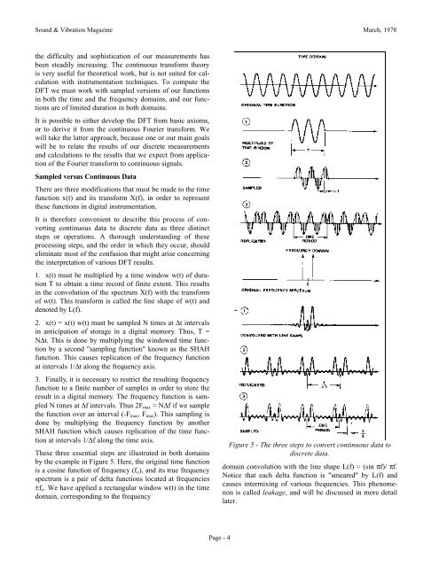
1. x(t) must be multiplied by a time window w(t) of duration
T to obtain a time record of finite extent. This results
in the convolution of the spectrum X(f) with the transform
of w(t). This transform is called the line shape of w(t) and
denoted by L(f).
2. x(t) = x(t) w(t) must be sampled N times at Δt intervals
in anticipation of storage in a digital memory. Thus, T =
NΔt. This is done by multiplying the windowed time function
by a second "sampling function" known as the SHAH
function. This causes replication of the frequency function
at intervals 1/Δt along the frequency axis.
3. Finally, it is necessary to restrict the resulting frequency
function to a finite number of samples in order to store the
result in a digital memory. The frequency function is sampled
N times at Δf intervals. Thus 2Fmax = NΔf if we sample
the function over an interval (-Fmax, Fmax). This sampling is
done by multiplying the frequency function by another
SHAH function which causes replication of the time function
at intervals 1/Δf along the time axis.
These three essential steps are illustrated in both domains
by the example in Figure 5. Here, the original time function
is a cosine function of frequency (fo), and its true frequency
spectrum is a pair of delta functions located at frequencies
±fo. We have applied a rectangular window w(t) in the time
domain, corresponding to the frequency
Page - 4
Figure 5 - The three steps to convert continuous data to
discrete data.
domain convolution with the line shape L(f) = (sin πf)/ πf.
Notice that each delta function is "smeared" by L(f) and
causes intermixing of various frequencies. This phenomenon
is called leakage, and will be discussed in more detail
later.