Superbus Positioning System A High Accuracy Networked ... - TU Delft
Superbus Positioning System A High Accuracy Networked ... - TU Delft
Superbus Positioning System A High Accuracy Networked ... - TU Delft

Create successful ePaper yourself
Turn your PDF publications into a flip-book with our unique Google optimized e-Paper software.
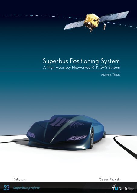
<strong>Delft</strong>, 2010<br />
<strong>Superbus</strong> <strong>Positioning</strong> <strong>System</strong><br />
A <strong>High</strong> <strong>Accuracy</strong> <strong>Networked</strong> RTK GPS <strong>System</strong><br />
Master’s Thesis<br />
Gert-Jan Pauwels
<strong>Superbus</strong> <strong>Positioning</strong> <strong>System</strong><br />
A <strong>High</strong> <strong>Accuracy</strong> <strong>Networked</strong> RTK GPS <strong>System</strong><br />
MASTER OF SCIENCE THESIS<br />
For obtaining the degree of Master of Science in Aerospace<br />
Engineering at <strong>Delft</strong> University of Technology<br />
Gert-Jan Pauwels<br />
1097407<br />
March 7, 2011<br />
Faculty of Aerospace Engineering · <strong>Delft</strong> University of Technology
Copyright c○ Gert-Jan Pauwels<br />
All rights reserved.
DELFT UNIVERSITY OF TECHNOLOGY<br />
CHAIR OF<br />
MATHEMATICAL GEODESY AND POSITIONING (MGP)<br />
The undersigned hereby certify that they have read and recommend to the Faculty<br />
of Aerospace Engineering for acceptance a thesis entitled “<strong>Superbus</strong> <strong>Positioning</strong> <strong>System</strong>”<br />
by Gert-Jan Pauwels in partial fulfillment of the requirements for the degree of<br />
Master of Science.<br />
Head of chair MGP:<br />
Supervisor:<br />
Supervisor:<br />
Dated: March 7, 2011<br />
prof.dr.ir. R.F. Hanssen<br />
dr.ir. Christian Tiberius<br />
Dr. Antonia Terzi
Acknowledgements<br />
The road I took during the making of this thesis, has had me thinking frequently<br />
of the tortoise and the hare parable. I have come to the conclusion that a third creature<br />
should’ve entered the race. I propose a creature not necessarily as slow as a tortoise,<br />
however with a horrible sense of direction. Eventually stumbling across the finish<br />
line, having completely forgotten he had entered a race, yet having seen and learnt a<br />
lot. This would illustrate somewhat how I have come to this thesis. A lot of different<br />
things have kept me busy during the making of this thesis, sometimes losing sight of<br />
what was happening around me, but learning a great many things. Therefore, to start<br />
of, I would like to thank everybody, that has aided me during the process, and sometimes<br />
pointed me back in the right direction. It has been truly interesting, fun, and very<br />
informative.<br />
I would like to thank Christian, of course, for his enthusiasm and helping me in<br />
such a way, that I still had to think about what it was I had to do. I have walked out of<br />
your office many times, thinking I knew the answer, only to discover, it wasn’t quite<br />
as straight forward as it seemed. I would like to thank you sincerely for making this<br />
thesis an enjoyable experience. I would also like to thank the whole <strong>Superbus</strong> team,<br />
especially Antonia and Maarten, for the infrequent but highly enjoyable contact, and<br />
giving me the opportunity to help you with the <strong>Superbus</strong>. The freedom and responsibility<br />
you have given me in the making of this system, is greatly appreciated. Furthermore<br />
I would like to thank Lennard for teaching me the practical skills of playing around<br />
with expensive equipment. This was a lot of fun, and has been essential to turn theory<br />
into practise and the other way around. This gratitude is also directed towards Roel,<br />
who has given me a beautiful opportunity for a test campaign, and helping me a lot in<br />
the process. Frank Boon from Septentrio is also thanked, in particular for the speed<br />
and remarkable openness of the responses from him and his company.<br />
My sincere gratitude also goes out to all my friends and family, for helping me and<br />
always being there. You have given me the confidence and perseverance to complete<br />
this study. This would not have been possible otherwise. I hesitate naming you all<br />
in person, in fear of forgetting or ranking anyone. Certainly my parents deserve an<br />
honourable mentioning. They have given me opportunities that not many people have,<br />
for which I am extremely grateful. Also specifically for helping me the last few hectic<br />
months with proofreading and logistic tasks. My brother also, for sometimes carving<br />
my path, and sometimes the pointy but truthful remarks. A special thanks also to<br />
Dennis, for helping me with the visual lay out of the report and presentation. Son, Ro,<br />
Behn, Nigel, Michiel, Matthijs, Klaas, Jelle, Geert, David, Daf, Joep, Barend, Noortje,<br />
Floor, Nathalie, Elisa, Claire, Doris, Lysanne, Vi and all the others, thanks for all the<br />
pep talks/proofreading/dinners/climbing and all the other forms of help and activities.<br />
It was great.
Abstract<br />
In this report a high accuracy positioning system is investigated for use in the <strong>Superbus</strong>.<br />
The <strong>Superbus</strong> project is an effort to apply a new and complete conceptual<br />
approach to public transport. It consists of a vehicle, logistics and infrastructure. The<br />
positioning system for the vehicle is to have a horizontal position error, which will not<br />
exceed 5 cm in 95% of the obtained solutions. Secondary requirements included large<br />
(quasi-national) deployment area. <strong>Networked</strong> RTK positioning using GPS is shown to<br />
be a valid means to adhere to these requirements. Real Time kinematic (RTK) positioning<br />
allows for the required accuracy, while a base station network will allow for<br />
the required deployment area using Pseudo Reference Stations (PRS). UMTS is shown<br />
to be potentially effective for the required wireless data transfer using the NTRIP protocol.<br />
Testing confirmed adherence of the <strong>Superbus</strong> <strong>Positioning</strong> <strong>System</strong> to the requirements<br />
in a variety of real world scenarios. Furthermore, the receiver is shown<br />
to perform to manufacturer specifications. Difficult environmental conditions, such as<br />
urban areas and multipath are confirmed to have an effect on the position estimate in<br />
certain situations. It is however demonstrated that the receiver is capable of adhering<br />
to <strong>Superbus</strong> requirements in these situations, provided the initial ambiguity resolution<br />
is correct. Temporary signal loss of all satellites (for example due to an underpass)<br />
is shown to inflict the need to reinitialise the ambiguity resolution algorithm, causing<br />
a temporary unavailability (around 20 seconds) of the precise RTK position estimate.<br />
Heading estimates are also established to be within specifications in good conditions.<br />
In high multipath conditions, or conditions with a low amount of satellites in view, the<br />
heading estimates exceed the manufacturing specifications with varying margins. This<br />
is possibly due to the fact that the ambiguities of the secondary antenna cannot be fixed<br />
in this scenario. Material testing showed that carbon fibre, the material that initially<br />
would cover the antennas in the vehicle, is highly unfit for this purpose.<br />
iii
Preface<br />
Writing a preface is a strangely personal affair. It is one of the last things one does,<br />
before print. A lot of things that have occupied you during the making of the report<br />
often find a way in the text. For this reason, I have decided to write this part in Dutch.<br />
Some have (rightfully) commented that the text below is quite easily translatable in<br />
English. Still, I have opted to keep it this way, since the language is closest to me, and<br />
the majority of the people that will read this. I apologise to the people who are not able<br />
to read the preface, but I hope that they will enjoy the rest of the thesis.<br />
Tijdens mijn scriptie is mij vaak gevraagd, wat de <strong>Superbus</strong> nu precies is. Één van<br />
mijn antwoorden was vaak, dat het een demonstratie was van de stand van de wetenschap.<br />
Wat is er mogelijk met wetenschap, en waar gaat het naartoe. Techniek, zoals<br />
de <strong>Superbus</strong>, is bij uitstek een graadmeter voor de stand van de wetenschap omdat het<br />
aantoont wat voor de mens beheersbaar is geworden. Dit beheersbare element is een<br />
steunpilaar, een wetenschappelijke theorie moet falsifieerbaar zijn. Techniek is niet<br />
mogelijk zonder dat de uitkomst van een actie voorspelbaar is. Dit klinkt logisch, toch<br />
is wetenschap niet altijd verbonden geweest met falsificatie. Descartes heeft dit in<br />
1637 als eerste opgeschreven in zijn Discours de la Méthode [8]. Dit wil niet zeggen<br />
dat er daarvoor geen nuttige dingen zijn gezegd of uitgevonden, maar wel dat sindsdien<br />
de kijk op de wereld en de wetenschap is veranderd. In de volgende paragrafen<br />
zal hier los op worden ingegaan [35].<br />
In de vorige paragraaf zijn een aantal dingen impliciet opgenomen. Één daarvan<br />
is dat techniek klaarblijkelijk evolueert. Dit Darwinisme is een vreemd fenomeen,<br />
en het laatste -isme, dat door de moderne wetenschap wordt zonder hakken en stoten<br />
wordt geaccepteerd. De moderne samenleving ervan doordrenkt. Het kernpunt van<br />
het Darwinisme, van evolutie, is een gebroken eenheid. het hangt aan elkaar door<br />
sterfelijkheid, vermenigvuldiging en verandering. Een nakomeling is een replicatie<br />
van zijn ouders. Deze mens niet hetzelfde als zijn ouders, maar men spreekt wel over<br />
hetzelfde, een mens. Mijn opa is gestorven, dat zal ik ook. Wij zijn niet hetzelfde,<br />
toch dragen wij dezelfde naam. Wij delen een identiteit, die groter is dan wij als individuen.<br />
Ondanks dat een paard door de jaren heen is veranderd, blijft men spreken<br />
van een paard. Identiteit is veranderlijk, en wordt pas, juist door zijn vermenigvuldiging<br />
duidelijk. Darwinisme betekent een verandering van de kleinste gemene deler van<br />
hetzelfde. Deze is met het Darwinisme omgewenteld van individu naar genoom.<br />
Als gezegd viert Darwinisme hoogtij. Dit is omdat met de ontdekking van het<br />
Darwinisme zeer veel wordt blootgelegd in taal, cultuur en techniek. het extended<br />
phenotype van de mens [7]. Taal bestaat ook uit een gebroken eenheid. De betekenis<br />
wordt duidelijk door zijn vermenigvuldiging, tevens is de identiteit ervan evengoed<br />
veranderlijk. Een woord dat slechts eenmaal wordt gebruikt, is betekenisloos. Tevens<br />
kan een woord kan uitsterven, en een betekenis kan veranderen. Wij gaan er vaak vanuit<br />
dat taal utilitaristisch is, dat wij controle hebben over de taal. Dit kun je niet meer<br />
volhouden wanneer je het bovenstaande accepteert. Voorbeeld, een kind voegt zich in,<br />
in de heersende taal. Deze is groter dan zichzelf, en hierdoor wordt het onmogelijk om<br />
v
vi<br />
”om het hoekje” van je eigen taal te kijken. Je bent al ingelijfd in de taal, voordat je<br />
er over wilt praten. Dit illustreert dat techniek cultuur en taal met de mens leven, maar<br />
dat de mens geen controle heeft over het verloop ervan. Dit ligt aan alle heersende<br />
omstandigheden.<br />
Is de mens hier niet de factor die besluit wat juist en onjuist is? Is ze niet de ratio<br />
van techniek? Een gedachte experiment. Het betreft de vraag waar ratio en betekenis<br />
op komen zetten. Wat betekent iets, en daarmee, wat is iets. Het kan vrij simpel<br />
worden verwoord. Stel wij hebben twee simpele en gelijkende organismen A en B. B<br />
wijkt op een cruciaal punt af van A, doordat B de mogelijkheid heeft een verandering<br />
in zuurgraad te detecteren. Hierdoor heeft B de mogelijkheid om zich uit de voeten<br />
te maken als het heersende milieu hem niet zint, waarbij A zich overlevert aan pure<br />
kans. B vergroot hiermee zijn overlevingskans en zal ter zijner tijd zege vieren in het<br />
gevecht om dezelfde, beperkte levensomgeving.<br />
Het is belangrijk te zien dat door deze ontwikkeling een betekeniswereld wordt<br />
geopend. Het is plotsklaps zinvol geworden om over zuur en niet zuur te praten. Het<br />
beïnvloed je overlevingskansen. Daarvoor kon je niet spreken over zuur en niet zuur.<br />
Er was geen verschil tussen, het was betekenisloos. Met de mogelijkheid tot detectie,<br />
ontstaat zuurtegraad, plaats en tijd, juist doordat er consequenties aan zijn verbonden.<br />
Hiermee wordt duidelijk dat een replicator (genoom) een ratio heeft boven die van<br />
het individu (replicant). Je kunt niet anders dan zeggen dat het genoom van soort B (per<br />
toeval) rationeel is geweest. De ontwikkeling was het goede antwoord op de heersende<br />
omstandigheden. Soort A heeft verloren, soort B leeft voort. Zo is de ontwikkeling<br />
van de vleugel ook een juist antwoord op de heersende omstandigheden. Stukje bij<br />
beetje heeft zich dat steeds verder ontwikkeld tot iets waarmee een vogel kan vliegen.<br />
De uitkomst had ook niet iets anders kunnen zijn dan iets wat lift genereert, want een<br />
vleugel moet zich houden aan de wetten van de wereld om zich heen. Je kunt dus<br />
ook niet anders zeggen, dan dat een vleugel er is om te vliegen. Het is onlosmakelijk<br />
verbonden aan zijn functie. De natuur heeft het bij het rechte eind.<br />
Dit kan geëxtrapoleerd worden naar techniek. Een hamer (ook een replicator)<br />
heeft zich in de geschiedenis ontwikkeld en is immer bijgebleven met de heersende<br />
omstandigheden. De botte steen is uitgestorven, en de hout met stalen constructie leeft<br />
voort, daar ze het meest passend is voor de heersende omstandigheden. Het woord<br />
hamer blijft, de fysieke verschijning ervan verandert.<br />
Ook voor wetenschap geldt hetzelfde. Teruggrijpend op de geschiedenis: Descartes<br />
kwam zoals eerder vermeld, met de wetenschappelijke methode. Een manier voor het<br />
bedrijven van wetenschap. Falsifieerbaarheid kwam hiermee hoog in het vaandel. Dit<br />
duidde op een eerste radicale omwenteling van het wereldbeeld: de mechanisering<br />
(de tweede is het Darwinisme). het was een omwenteling in de identiteit van dingen.<br />
Het veranderde de blik van wat iets is en maakte het onafhankelijk van geloof (bijvoorbeeld<br />
de Ideeënleer van Plato met een niet fysieke wereld met de essentie van<br />
álle dingen erin) en trok het naar reproduceerbaarheid. Water was niet meer per s een<br />
stof met een essentie. Neen, water is een stof die gaat koken bij honderd graden. De
eigenschap kun je reproduceren, en gebruiken. Maar belangrijker: Een tripje naar de<br />
alpen maakt het tegendeel duidelijk. Toch, de wet is niet ongeldig geworden door<br />
een tegenspraak. Ze is er tegen bestand. Ze is ingedekt om tegenstand te weerstaan,<br />
kan veranderen en variaties in zich opnemen, naar mate de wetenschap voort schrijdt.<br />
Een hypothese blijft bestaan als ze de beste resultaten oplevert. Iets is hiermee bij zegen<br />
van zijn reproduceerbaarheid en de potentiële gebruiken ervan. De wetten die dit<br />
beschrijven zijn ook onderhevig aan het Darwinisme. Slechts de meest passende hypotheses<br />
zullen overleven in de strijd van de wetenschap. herinnert u zich Phlogiston<br />
nog?<br />
Descartes zei het onopgemerkt zelf al. Hij probeerde, levend in het tweespalt<br />
tussen klassieke en wetenschappelijke wereld, nog een opening te houden voor klassieke<br />
opvattingen, maar daar faalt hij in. Hij zag de wetenschap als boom [9]. Met een dikke<br />
stronk, en uitbreidend in steeds kleiner wordende takken. De stronk was voor hem<br />
de basiswetenschap, wiskunde en fysica. Van daaruit kon elke wetenschap en kennis<br />
worden afgeleid, de steeds maar kleiner worden takken. Hij doorzag echter al dat elke<br />
wetenschappelijke hypothese uiteindelijk wordt getoetst uit de techniek die het voort<br />
brengt: de vruchten. Deze techniek dicht het gat tussen mens en natuur, met wielen,<br />
hamers, telefoons en internet. Deze vruchten zijn succesvol. De vruchten voeden<br />
daarmee de boom voor de immer voortschrijdende wetenschap. Wederom Becher met<br />
zijn Phlogiston. Zijn simpele elementen systeem was op de lange duur niet afdoende<br />
meer, de tak baarde op den duur minder vruchten dan concurrerende hypotheses, en<br />
storf af. Ze is nutteloos geworden<br />
Descartes, in zijn tweespalt, kon zijn boom echter niet in de lucht laten zweven, en<br />
zocht naarstig naar een (naar het blijkt onnodige) grond voor de wortels. Deze grond<br />
vond hij in de religie en de filosofie (metafysica). Hiermee voert hij helaas een totaal<br />
overbodige dubbele boekhouding in. Zijn theologische en filosofische gronden voor de<br />
wetenschap zijn onnodig wanneer het succes van een wetenschap slechts beoordeeld<br />
wordt uit het resultaat.<br />
Waar komt <strong>Superbus</strong> in dit verhaal? Dat kan alleen de toekomst vertellen. De<br />
identiteit van de superbus moet nog duidelijk worden. Duidelijk is wel dat het een<br />
mooi voorbeeld is van het resultaat van de wetenschap. Bij uitstek een voorbeeld van<br />
waarom ik techniek ben gaan studeren. Een apparaat dat ogenschijnlijk de wetenschap<br />
tart. Over enkele jaren zullen we niet meer verbaasd zijn over dit project. Dan wekken<br />
andere dingen onze interesse, oud nieuws. Dat wil niet zeggen dat de <strong>Superbus</strong> vergeten<br />
is. Dat ligt eraan of <strong>Superbus</strong> een succesvolle replicator gaat worden.<br />
vii
Contents<br />
Contents ix<br />
List of Figures xi<br />
1 Introduction 1<br />
2 <strong>Superbus</strong> 3<br />
2.1 The <strong>Superbus</strong> project . . . . . . . . . . . . . . . . . . . . . . . . . . 3<br />
2.2 Conceptual design . . . . . . . . . . . . . . . . . . . . . . . . . . . . 6<br />
2.3 <strong>Superbus</strong> and positioning . . . . . . . . . . . . . . . . . . . . . . . . 13<br />
2.4 <strong>Superbus</strong> positioning requirements . . . . . . . . . . . . . . . . . . . 13<br />
2.5 <strong>Superbus</strong> positioning project definition . . . . . . . . . . . . . . . . . 14<br />
3 Theory Of <strong>High</strong> <strong>Accuracy</strong> GPS 17<br />
3.1 GPS . . . . . . . . . . . . . . . . . . . . . . . . . . . . . . . . . . . 17<br />
3.2 Standard <strong>Positioning</strong> Service . . . . . . . . . . . . . . . . . . . . . . 22<br />
3.3 Measurement error sources . . . . . . . . . . . . . . . . . . . . . . . 26<br />
3.4 Augmented positioning . . . . . . . . . . . . . . . . . . . . . . . . . 28<br />
3.5 The LAMBDA method and future enhancements . . . . . . . . . . . 39<br />
3.6 Pseudorange rates . . . . . . . . . . . . . . . . . . . . . . . . . . . . 43<br />
3.7 Communication . . . . . . . . . . . . . . . . . . . . . . . . . . . . . 45<br />
3.8 Concluding remarks . . . . . . . . . . . . . . . . . . . . . . . . . . . 51<br />
4 <strong>Superbus</strong> <strong>Positioning</strong> <strong>System</strong> 55<br />
4.1 Introduction to the <strong>Superbus</strong> <strong>Positioning</strong> <strong>System</strong> . . . . . . . . . . . . 55<br />
4.2 NTRIP . . . . . . . . . . . . . . . . . . . . . . . . . . . . . . . . . . 56<br />
4.3 <strong>Superbus</strong> <strong>Positioning</strong> <strong>System</strong> . . . . . . . . . . . . . . . . . . . . . . 57<br />
4.4 The Position Module . . . . . . . . . . . . . . . . . . . . . . . . . . 64<br />
4.5 GPS applications and future developments . . . . . . . . . . . . . . . 71<br />
5 Validation of <strong>Superbus</strong> <strong>Positioning</strong> <strong>System</strong> 79<br />
5.1 Introduction to validation . . . . . . . . . . . . . . . . . . . . . . . . 79<br />
5.2 Performance requirements . . . . . . . . . . . . . . . . . . . . . . . 84<br />
5.3 Experiments . . . . . . . . . . . . . . . . . . . . . . . . . . . . . . . 86<br />
ix
x CONTENTS<br />
5.4 Test results . . . . . . . . . . . . . . . . . . . . . . . . . . . . . . . 98<br />
6 Conclusion 135<br />
7 Discussion and Recommendations 139<br />
Bibliography 143<br />
Acronyms 149<br />
Appendices 153<br />
A Septentrio PolaRx2e Specifications 155<br />
B Septentrio PolaNt Specifications 159<br />
C Antenna radiation pattern 161<br />
D Example output Position Module 165<br />
E Angular velocity precision estimation 169
List of Figures<br />
2.1 Front and side view of a <strong>Superbus</strong> vehicle. [source: <strong>Superbus</strong>] . . . . . . 5<br />
2.2 Comparison between a <strong>Superbus</strong> and a conventional bus. [source: <strong>Superbus</strong>] 10<br />
2.3 Gull-wing door design. [source: <strong>Superbus</strong>] . . . . . . . . . . . . . . . . . 11<br />
2.4 Ground clearance in high and low settings. [source: <strong>Superbus</strong>] . . . . . . 11<br />
3.1 Segments of the GPS system. [source: NATIONAL ACADEMY PRESS<br />
[2]] . . . . . . . . . . . . . . . . . . . . . . . . . . . . . . . . . . . . . 18<br />
3.2 Graphical representation of a multipath situation. [source: BKG] . . . . . 27<br />
3.3 Graphical representation of an RTK set up. . . . . . . . . . . . . . . . . . 33<br />
3.4 Graphical representation of relative positioning errors. [Source: 06-GPS] 38<br />
3.5 2D example constant cost ellipsoids before (a) and after (b) the decorrelation<br />
step. Rounding in the first scenario would produce incorrect integers<br />
of (4,5), while rounding in the second scenario produces the correct<br />
(−2,10). [Source: [31]] . . . . . . . . . . . . . . . . . . . . . . . . . . . 41<br />
3.6 Cell structure of cellular networks. [source: [5]] . . . . . . . . . . . . . . 48<br />
3.7 Representation of frequency shift modulation. [source: wikipedia] . . . . 48<br />
4.1 Generic NTRIP set up. . . . . . . . . . . . . . . . . . . . . . . . . . . . 58<br />
4.2 <strong>Superbus</strong> GPS system lay out with dedicated base station. . . . . . . . . . 60<br />
4.3 <strong>Superbus</strong> GPS system lay out with network based VRS. . . . . . . . . . . 62<br />
4.4 Septentrio PolaNt antenna and the PolaRx2eH receiver. [source: Septentrio] 63<br />
4.5 Placement of the two GPS antennas in the <strong>Superbus</strong>. . . . . . . . . . . . 65<br />
4.6 Position Module, high level lay out. . . . . . . . . . . . . . . . . . . . . 67<br />
4.7 Vehicle behaviour during cornering. Active suspension is enabled on the<br />
right. [source: Bose] . . . . . . . . . . . . . . . . . . . . . . . . . . . . 72<br />
4.8 <strong>Superbus</strong> FMS example. . . . . . . . . . . . . . . . . . . . . . . . . . . 76<br />
5.1 Bias and precision graphically represented, accuracy = precision + bias.<br />
[source: wikipedia] . . . . . . . . . . . . . . . . . . . . . . . . . . . . . 81<br />
5.2 Outlier detection. [source: Septentrio] . . . . . . . . . . . . . . . . . . . 82<br />
5.3 Location of the material test. [source: Google Earth] . . . . . . . . . . . 88<br />
5.4 Number of satellites visible during materials test (cut-off angle 5 ◦ ). . . . . 88<br />
xi
xii List of Figures<br />
5.5 Rover antenna covered with carbon fibre material,supported by the wooden<br />
construction. . . . . . . . . . . . . . . . . . . . . . . . . . . . . . . . . . 90<br />
5.6 NMIbuilding and test set up. . . . . . . . . . . . . . . . . . . . . . . . . 91<br />
5.7 Overview of the top of the NMI building. . . . . . . . . . . . . . . . . . 91<br />
5.8 Vehicle frame overview, dimensions and antenna placement. Vehicle front<br />
is top of figure. . . . . . . . . . . . . . . . . . . . . . . . . . . . . . . . 94<br />
5.9 Vehicle with installed frame. . . . . . . . . . . . . . . . . . . . . . . . . 96<br />
5.10 Skyplot over <strong>Delft</strong>, during the materials experiment. . . . . . . . . . . . . 98<br />
5.11 Comparison of three, 30 minute, static solutions. . . . . . . . . . . . . . 99<br />
5.12 Comparison of the dynamic solutions. . . . . . . . . . . . . . . . . . . . 102<br />
5.12 Comparison of the dynamic solutions. . . . . . . . . . . . . . . . . . . . 103<br />
5.13 C/N0 (signal strength) ratios of two satellites under three circumstances. . 104<br />
5.14 Skyplot over <strong>Delft</strong>, during the static experiment. . . . . . . . . . . . . . . 105<br />
5.15 X position and heading error over time. . . . . . . . . . . . . . . . . . . 106<br />
5.16 Speed error over time. . . . . . . . . . . . . . . . . . . . . . . . . . . . . 107<br />
5.17 Skyplot over <strong>Delft</strong>, during the reacquisition experiment . . . . . . . . . . 108<br />
5.18 Demonstration of incorrect RTK ambiguity fix. . . . . . . . . . . . . . . 108<br />
5.19 Heading error due to unfixed secondary antenna. . . . . . . . . . . . . . 110<br />
5.20 Detail: Divergent heading error before loss of RTK. . . . . . . . . . . . . 110<br />
5.21 Histogram of the reacquisition times. A total of 56 trials . . . . . . . . . 111<br />
5.22 Cumulative representation of reacquisition times. . . . . . . . . . . . . . 112<br />
5.23 Track of the Duifpolder experiment. [source: Google earth] . . . . . . . . 112<br />
5.24 Skyplot over <strong>Delft</strong>, during the Duifpolder experiment. . . . . . . . . . . . 113<br />
5.25 Position error in relation to PVT Mode. . . . . . . . . . . . . . . . . . . 118<br />
5.26 Heading error in relation to PVTMode and NrSV. . . . . . . . . . . . . . 120<br />
5.27 Receiver speed comparison of the Duifpolder experiment. . . . . . . . . . 121<br />
5.28 Septentrio speed in relation to heading errors. . . . . . . . . . . . . . . . 121<br />
5.29 Track of the Emerald experiment. [source:Google Earth] . . . . . . . . . 122<br />
5.30 Skyplot over <strong>Delft</strong>, during the Emerald experiment. . . . . . . . . . . . . 123<br />
5.31 Septentrio error to ground truth in relation to the PVT Mode. . . . . . . . 124<br />
5.32 Septentrio loss of solution behaviour. . . . . . . . . . . . . . . . . . . . . 125<br />
5.33 Heading error in relation to the NrSV and PVT Mode. . . . . . . . . . . . 126<br />
5.34 Heading error in relation to the NrSV and Velocity. . . . . . . . . . . . . 126<br />
5.35 Heading error detail, showing dependence to the NrSV. . . . . . . . . . . 127<br />
5.36 Heading error detail, showing dependence to the NrSV. . . . . . . . . . . 127<br />
5.37 Track of the A4 experiment. A Viaduct is present at the bottom of the<br />
track, an aqueduct crosses the halfway point of the track. [source: Google<br />
earth] . . . . . . . . . . . . . . . . . . . . . . . . . . . . . . . . . . . . 130<br />
5.38 Skyplot over <strong>Delft</strong>, during the A4 experiment. . . . . . . . . . . . . . . . 130<br />
5.39 Total Position error during A4 with respect to PVT Mode. . . . . . . . . . 131<br />
5.40 Cumulative time to first fix probabilities, absolute and RTK fixed. . . . . 132<br />
5.41 Heading errors versus PVT Mode and Number of satellites in view. . . . . 134<br />
E.1 Angular velocities as experienced by the <strong>Superbus</strong>. . . . . . . . . . . . . 169
Chapter 1<br />
Introduction<br />
For several decades now, the major cities in the west of the Netherlands have been<br />
growing steadily in prosperity and population, while the north of the country has seen<br />
a relatively slower growth. Especially in times of a beneficial economic climate the<br />
growth of the northern provinces has been lagging behind. In 1997 this was also the<br />
conclusion of a government commission that suggested that the profits, gained from<br />
the vast gas deposits of the north, could be used to improve infrastructure in these<br />
areas. One of the incentives involves a better and faster transportation link between<br />
the west and the north of Holland. By doing this, the hope is that the northern cities<br />
will start to see larger economic growth figures, due to much faster and easier traffic<br />
between the north and the economic heart of the west.<br />
The <strong>Superbus</strong> project started in 2004 as a reaction to this incentive, as well as to<br />
other modern day environmental and mobility issues: pollution, congestion and safety.<br />
The <strong>Superbus</strong> project sees to tackle these issues by applying a new and complete conceptual<br />
approach to public transport. It consists of a vehicle, but also new dedicated<br />
infrastructure and new logistics.<br />
The <strong>Superbus</strong> itself is a high tech, road going vehicle that has been designed to be<br />
fast, safe, comfortable, and flexible in order to promote its usability. Furthermore it<br />
has been designed to have as little environmental impact as possible. It is to attain a<br />
cruising speed of 250 km/h and will be powered electrically.<br />
With the technology present in the vehicle, a demand also followed for a real time,<br />
high accuracy positioning system. Requirements were set according to which the horizontal<br />
position error of the system may not exceed 5 cm in 95% of the obtained solutions.<br />
This system will allow <strong>Superbus</strong> subsystems to function optimally and can<br />
allow for more advanced future upgrades, to the vehicle and the whole <strong>Superbus</strong> system.<br />
The purpose of this report is to investigate a positioning system, that can adhere<br />
to the requirements set by <strong>Superbus</strong>. Additionally the designed system will be tested<br />
to validate it’s suitability for use in the vehicle.<br />
The structural composition of the report is as follows. Chapter 2 will serve as an<br />
introduction to the <strong>Superbus</strong>, and the project as a whole. <strong>System</strong> requirements will<br />
1
2 CHAPTER 1. INTRODUCTION<br />
be specified, and the project goals will be defined precisely. Chapter 3 will constitute<br />
a theoretical background to the project, and will explain what systems are necessary.<br />
Chapter 4 will describe the positioning system and its practicalities. Chapter 5 will<br />
serve as the main chapter wherein the obtained system is tested and validated. The last<br />
two chapters will consist of a conclusion, discussion and of recommendations.
Chapter 2<br />
<strong>Superbus</strong><br />
Public transport plays an important role in modern society, it has become a backbone<br />
for both social and economic interaction. This infusion in society does however not<br />
mean that changes and improvements in public transport are not possible or desirable.<br />
This is the vision of the <strong>Superbus</strong> project, it aims to re-establish the way we look at<br />
public transport.<br />
This chapter will function as an introduction to the <strong>Superbus</strong> project. The origin of<br />
the project will be considered shortly, and <strong>Superbus</strong> concept will be introduced. In the<br />
subsequent sections an introduction to <strong>Superbus</strong> positioning will be made, after which<br />
the requirements and positioning project will be defined.<br />
2.1 The <strong>Superbus</strong> project<br />
The <strong>Superbus</strong> project started in 2004 as a reaction to modern day environmental and<br />
mobility issues: pollution, congestion, time constraints and safety. These are issues<br />
that gained tremendously in importance in the last decade. The project will try to<br />
tackle these mobility issues from more than one perspective. The project really took<br />
off in November of 2005 when it received a grant from the Ministry of Transport, Public<br />
works and Water management (Ministerie van Verkeer en Waterstaat), currently the<br />
Ministry of Infrastructure and Environment. The grant was conceived for the development<br />
of a means of public transport between the north of the Netherlands and the<br />
more densely populated south-west. This means of transport should function as an<br />
economic and social catalyst to draw the historically more isolated northern part of the<br />
Netherlands and the south-west closer to each other. <strong>Superbus</strong> was one such means of<br />
transport selected that could fulfil this role.<br />
After the grant was received, the detailed development got underway and in the beginning<br />
of 2007 construction began on a first test vehicle. Development of the detailed<br />
design continued throughout the building process, which is now nearly complete. After<br />
its completion the vehicle will undergo rigorous testing to analyse performance<br />
and ensure passenger safety. During this time <strong>Superbus</strong> will try to develop enough<br />
3
4 CHAPTER 2. SUPERBUS<br />
knowledge and momentum for the concept to make implementation of the concept a<br />
possibility.<br />
The <strong>Superbus</strong> project is a project that tries to rethink public transport. The goal of<br />
the project to provide a fast, demand based road transportation system for medium to<br />
longer distances up to approximately 250 kilometres. It tries to address modern mobility<br />
demand with a fast, safe and environmentally friendly public transport vehicle.<br />
The vehicle is specifically designed with speed, passenger comfort and sustainability<br />
in mind. It is important to note that it is a complete conceptual approach to public<br />
transport, and as such the project does not constitute a transport vehicle alone. The<br />
<strong>Superbus</strong> project spreads over multiple disciplines:<br />
• Vehicle<br />
• Infrastructure<br />
• Logistics<br />
• Safety and Reliability<br />
• Environmental aspects<br />
• Exploitation and economic viability<br />
In order to discuss the concept of <strong>Superbus</strong>, the background is enlightened first.<br />
The demand for transportation grows constantly, as does the amount of people who<br />
demand it. People have been travelling further and further over the years, caused by<br />
technological advances. Yet for daily commutes, time is a more important factor than<br />
distance. People generally do not wish to spend more than a certain amount of time<br />
each day on transportation, or travelling [29]. This situation is now aggravated by an<br />
ever growing fleet of cars dressing the nation, causing bottlenecks and traffic jams in<br />
the established road network. Conventional growing of this infrastructure, building<br />
more roads for more cars, will not be a viable, sustainable solution to the problem.<br />
Not only due to space constraints, but also due to safety issues and pollution. <strong>Superbus</strong><br />
therefore tries to find one of the solutions to this problem. It does so by studying<br />
the reasons for people to take cars and tries to derive an feasible alternative. At the<br />
same time the solution must be sustainable, both for people and the environment.<br />
An important element is to find the appealing and deterring factors of both private<br />
and public transport. For example: the sense of privacy one has in a private vehicle, as<br />
well as the fact that one is able to drive right to the door of your destination, are compelling<br />
factors for a automobile. On the other hand, a person driving is not able to do<br />
work, for example. Public transport can in some cases allow for this, as well as avoid<br />
many known traffic bottlenecks. If a new form of public transport is to be successful it<br />
will need to outweigh the advantages of a car and/or negate the annoyances of public<br />
transport.<br />
It is clear that the problem has multiple facets, there is no single source that causes<br />
the problem. As mentioned, the <strong>Superbus</strong> project sees the solution in several facets as
2.1. THE SUPERBUS PROJECT 5<br />
well. For example: moderating the overall road congestion by diminishing the number<br />
of vehicles on the road, increasing comfort and adding speed. The aspects mentioned<br />
in section 2.1, will all be combined to a system that is designed to provide fast, easy,<br />
comfortable and sustainable mobility to the user.<br />
Very concisely: <strong>Superbus</strong> consists of a vehicle together with infrastructure and is<br />
designed as a more flexible yet fast alternative (mainly) to modern high speed transport.<br />
It aims to be more flexible by applying an on-demand structure, in contrast to, or<br />
together with a normal time-table. Starting points and destinations are therefore more<br />
flexible, and can be more local due to the ability of the vehicle to use normal roads in<br />
addition to its own infrastructure.<br />
The <strong>Superbus</strong> (figure 2.1) itself is an electrical vehicle which can transport up to<br />
23 passengers at a speed of up to 250 (Km/h). The vehicle will be powered by batteries<br />
and will make use of separate infrastructure to reach these high velocities, the<br />
Supertrack. Thanks to the low weight, low aerodynamic drag and rolling resistance<br />
the vehicle is very energy efficient. The absence of exhaust fumes and the low energy<br />
use also make the <strong>Superbus</strong> an environmental friendly way of transport.<br />
Figure 2.1: Front and side view of a <strong>Superbus</strong> vehicle. [source: <strong>Superbus</strong>]<br />
Passengers are able to book a fare by means of internet or telephone. A central<br />
booking system combines passengers for matching destination and departure points<br />
and offers several travel options. The passenger can then book the most suitable, and<br />
has a journey with little stops or transfers. Passengers are boarded on the <strong>Superbus</strong> in<br />
urban areas on normal public roads before the vehicle goes to the Supertrack where it<br />
travels at high speed until it almost reaches destination. Here it transfers to local roads
6 CHAPTER 2. SUPERBUS<br />
to let the passengers of close to their end destinations.<br />
This condensed section is of course not the complete report of the <strong>Superbus</strong> system.<br />
In the section below an overview of the concept will be sketched, clarifying problems,<br />
visions and design choices in no particular order. The sections will hopefully create an<br />
insight in, and understanding of the main design philosophies of the <strong>Superbus</strong> system.<br />
2.2 Conceptual design<br />
A basic view of the <strong>Superbus</strong> concept has been presented in the previous section.<br />
This shows only the final result, provided the project is successful. In the following<br />
sections, a more elaborate view will be laid down in no particular order. It can create an<br />
insight into the design decisions and increase the overall understanding of the concept.<br />
Information for this section is redacted from <strong>Superbus</strong> documents [26–29, 52].<br />
Travel times<br />
First of all <strong>Superbus</strong> will try to reduce travel times in two ways. Not only does it<br />
increase the speed of motion compared to normal cars and trains, but it also tries to decrease<br />
transit,waiting, and initial transportation times (door-to-station). These can add<br />
up significantly in conventional public transport. The last method of reducing travel<br />
time is the use of dedicated <strong>Superbus</strong> infrastructure, Supertracks. These tracks allow<br />
the vehicle to reach its top cruising speeds, and circumvents normal traffic. In short,<br />
<strong>Superbus</strong> tries to reduce the door to door travelling times, not only the station to station<br />
times.<br />
With a cruising speed of 250 (km/h), <strong>Superbus</strong> will be competitive with most high<br />
speed train services. The travel times are additionally reduced by altering the conventional<br />
time tables and itineraries of classic public transport systems. These mainly<br />
employ fixed line services with predetermined stops. <strong>Superbus</strong> will employ an ondemand<br />
structure. This means that they are not bound to fixed time tables. Because<br />
the vehicle is not limited to tracks as are high speed trains, this means that they are<br />
also means that the fixed itinerary and destination becomes obsolete. The <strong>Superbus</strong><br />
will potentially be a much more flexible way of travel.<br />
The on-demand structure can be exploited to benefit the user. The user will be able<br />
to convey base and destination points to the <strong>Superbus</strong> system, as well as departureand<br />
or arrival times. The <strong>Superbus</strong> system is then able to pool multiple users together<br />
and devise a optimised itinerary which will minimise travel times. It will also avoid<br />
transits to a great extent, or optimise them, as to minimise the discomfort. The viability<br />
of such an on-demand system is aided by the fact the <strong>Superbus</strong> vehicle is able to<br />
carry a relatively low number of passengers for a public transportation vehicle: 20 to<br />
30 depending on the lay-out. This allows customisation of routes and travelling times,<br />
while still reducing the number of vehicles on the road significantly: A four person<br />
passenger car is on average only occupied by 1.4 people, a much smaller number than<br />
a <strong>Superbus</strong> [28].
2.2. CONCEP<strong>TU</strong>AL DESIGN 7<br />
Logistics<br />
Note that the <strong>Superbus</strong> will not be a pure door-to-door transportation vehicle. Collecting<br />
each passenger individually would take too much time and negate the time won by<br />
the speed of the vehicle. Yet by being fully road-going, stopping points can be much<br />
more dynamic than for example trains. These points are called concentration points.<br />
These can be created by introducing fixed stations, but they can always be dynamic<br />
as well: when- and wherever enough people are present to justify a stop, one can be<br />
created. Examples include events and conventions. Furthermore, because the <strong>Superbus</strong><br />
can only carry 20 to 30 people (depending on configuration), these concentration<br />
points can be relatively small and local.<br />
When the <strong>Superbus</strong> system is fully deployed and operational, it will employ a direct<br />
point to point routing system, with potentially a few local stops at the starting<br />
point and the destination. This will ensure fast travel times while maintaining a high<br />
degree of vehicle occupation and minimising the distance a user needs to travel to get<br />
onto the vehicle.<br />
This on-demand system does however not mean that standard line services will<br />
be ignored completely. If demand is stable and large enough, such a line service can<br />
be employed with little drawbacks, or even benefits, to the passenger. This can be<br />
of particular interest to commuters seeking for a stable fast way of travel for medium<br />
to long distances. An example here, might be the Zuiderzeelijn, the original route<br />
planned for the <strong>Superbus</strong>, mentioned in section 2.1. Also in the beginning roll out<br />
phase of the system, not enough vehicles will be available to employ an effective ondemand<br />
system. Additionally, the passenger base needs to have grown sufficiently<br />
large to support the system. This is a two way system that will need time to grow.<br />
One can see that if the concept takes off, the success will largely be dependent on<br />
modern ICT solutions. Managing many passengers individually, providing each with<br />
an efficient travel solution, but also managing an increasing <strong>Superbus</strong> fleet, including<br />
destination, route and current location, will need a new, highly optimised, highly converged,<br />
and continually up-to-date system. The old time table system is thrown out,<br />
yet it does need to be replaced with something superior to benefit the passenger. This<br />
in order to become a viable alternative to other forms of transport.<br />
Lastly the charter market may become a lucrative market for <strong>Superbus</strong>. Since the<br />
vehicle has a relatively low number of passengers, it becomes more obtainable for<br />
a single business to acquire a high occupancy rate (or load factor). At this point it<br />
may become beneficial to charter the complete vehicle. This will allow more freedom<br />
to the business and its users to travel on desired times and to desired destinations.<br />
This will again shorten travel times since the <strong>Superbus</strong> can use a direct route to the<br />
destination. This may especially be interesting to medium to large corporations with<br />
several branches within the range of the <strong>Superbus</strong>.
8 CHAPTER 2. SUPERBUS<br />
Passenger comfort and safety<br />
Benefits over other modes of transport, as already discussed in previous sections, are<br />
paramount for the success of the <strong>Superbus</strong> system. For example, the locality, and individuality<br />
of the <strong>Superbus</strong> approach mentioned above are important steps in the passenger’s<br />
perceived comfort, and likely diminish the reluctance to opt for public transport.<br />
The <strong>Superbus</strong> concept tries to do this in other areas as well.<br />
The vehicle itself will be extremely comfortable and is produced to express a certain<br />
luxury. It must offer a significant benefit over a car in order to convince people<br />
to take the <strong>Superbus</strong>. Therefore the seats are very comfortable and head- and legroom<br />
are very spacious. However, the sense of privacy in a car is not to be underestimated.<br />
The seats are spaced far apart and many individual entrances drape the vehicle for<br />
this reason. It will relieve some of the annoyances people perceive when using public<br />
transportation. People must not feel hindered while travelling, be it for privacy, comfort<br />
or the ability to work.<br />
The ride itself must also not be overlooked. A harsh journey can issue the same<br />
feeling and discomfort, and makes any form of productivity impossible for the passenger<br />
during the trip. First of all, the suspension design is a major factor for perceived<br />
comfort. Seconly, accelerations in all directions need to be managed: Longitudinal,<br />
lateral and vertical. This is shown in table 2.1.<br />
Table 2.1: Recommended acceleration domain. [Source: <strong>Superbus</strong> [28]]<br />
Direction domain (m/s 2 )<br />
Longitudinal ± 1.0<br />
Lateral ± 1.0<br />
vertical 9.31 - 10.81<br />
After analysis of comparable modes of transport, <strong>Superbus</strong> established that accelerations<br />
need to remain in this domain in order to be perceived as comfortable. There<br />
are several ways to achieve this. First and foremost, de- and acceleration should be<br />
kept within these limits during normal operation. <strong>Superbus</strong> will not be a race car: it<br />
will take a leisurely 70 seconds to accelerate from stand still to the cruising speed of<br />
250 (km/h) and vice versa. The vehicle is able to perform far better during emergency<br />
situations, but naturally these situations tend to be avoided.<br />
Lateral accelerations are harder to control, they are dependent on the speed of the<br />
vehicle and the radius of the turn, see equation 2.1. With a cruising speed of almost 70<br />
(m/s) this would leave a turn radius of 4.8 kilometres.<br />
a = (2.1)<br />
R<br />
The turning radius or speed can may be altered, if necessary, by banking the road.<br />
This will convert some of the lateral accelerations to vertical accelerations. This will<br />
V 2
2.2. CONCEP<strong>TU</strong>AL DESIGN 9<br />
allow tighter turns at greater speeds. Note that banking roads would on the other hand<br />
add to the cost of the infrastructure. Since one of the main advantages of the <strong>Superbus</strong><br />
concept is the relatively low infrastructural investment, this may need to be avoided.<br />
Another approach to this can be taken as well. In addition to the banking roads,<br />
the same results can be achieved by banking the vehicle: the same transition of forces<br />
applies. An active suspension system is able to raise, lower, soften and stiffen the suspension<br />
of each individual wheel. This would allow the vehicle to bank into the turn<br />
by raising the suspension on the outer wheels slightly. This will reduce the bank angle,<br />
and hence reduce the cost of the road. Note that this scenario is supposing the traction<br />
of the wheels is sufficient, and the aerodynamics are not disturbed beyond acceptable<br />
limits.<br />
The active suspension (atlhough currently not implemented) is useful for controlling<br />
vertical accelerations as well. Whenever a known coarseness in the road is encountered<br />
the suspension of the appropriate wheels can be softened moments prior, to<br />
allow the vehicle to coast over the unevenness due to the low weight of the wheel. This<br />
would significantly reduce the vertical accelerations, allowing the vehicle to remain at<br />
higher speeds while passing these variations in the road. This in turn would again reduce<br />
the cost of the infrastructure since the need for a perfectly even road is no longer<br />
there.<br />
All the measures mentioned above combined try to relieve the reluctance to take<br />
public transport and offer genuine advantages of choosing the <strong>Superbus</strong> over a normal<br />
car. But this comfort means very little without safety and reliability. Therefore safety<br />
is a priority both in infrastructure and in the vehicle itself.<br />
The fast Supertracks, the independent roads only accessible for <strong>Superbus</strong>, will be<br />
monitored actively. Cameras will control the entrances and fences or noise barriers<br />
will make access for wildlife and people difficult.<br />
The vehicle too will have many active safety features embedded. Computer systems<br />
will monitor more than 750 sensors, for example in the doors and seat belts of<br />
every passenger. These will affect the passengers directly. But all other on board parts<br />
and systems will be checked continuously as well. Tire pressure, engine and battery<br />
status, etc. Also seven radars will be fitted onto the <strong>Superbus</strong> to improve situational<br />
awareness. At 250 (km/h) it will take a significant length of road to stop, some 2.5<br />
kilometres. The radars will aid in detecting obstacles and irregularities before the pilot<br />
is able to, and can aid in taking appropriate action. Passive safety is also not forgotten.<br />
Mandatory seat belts were mentioned already but also the full carbon fibre body will,<br />
if necessary, protect the passengers.<br />
Sustainability<br />
Conservation of the environment has become a relevant issue in recent years, and as a<br />
result <strong>Superbus</strong> tries be as close to a environmentally neutral solution as possible. This<br />
will ideally serve as an incentive for others, and show that an environmentally viable
10 CHAPTER 2. SUPERBUS<br />
solution can also be an economically viable solution. Naturally, the low environmental<br />
impact will increase the marketability of the <strong>Superbus</strong> as well. Yet most importantly,<br />
it will ensure the <strong>Superbus</strong> will remain a viable option in the future, as legislation on<br />
carbon emissions and general environmental impact will invariably tighten.<br />
The vehicle itself is electrically powered and offers regenerative braking, in order<br />
to regain some of the kinetic energy of the vehicle. Electrical motors can convert energy<br />
to movement with greater efficiencies than conventional motors [28]. Also, the<br />
electrical energy can come from any number of (environmentally friendly) sources,<br />
wind, sun, etc. It is therefore less dependent on liquid fuel prices alone, in addition<br />
to being more efficient. Lastly, the aerodynamics are improved dramatically to reduce<br />
drag, and hence the power needed to attain the higher cruising speeds. The vehicle<br />
will approximately need the same power output at 250 km/h as a normal bus needs at<br />
100 km/h [28].<br />
To achieve the lower power requirement at speed, the frontal area is reduced in<br />
comparison with a conventional bus, and the aerodynamic properties are optimised<br />
to reduce the drag coefficient. This is can be seen in figure 2.2. By using advanced<br />
modelling and simulation software the drag coefficient has been reduced to one that is<br />
lower than a typical passenger car [28].<br />
Figure 2.2: Comparison between a <strong>Superbus</strong> and a conventional bus. [source: <strong>Superbus</strong>]<br />
The vehicle<br />
To allow for the high speed performance of the <strong>Superbus</strong> while still managing a reasonable<br />
power requirement, a low, light weight and aerodynamically efficient design<br />
is mandatory. This has consequences for the interaction with the vehicle.<br />
As can be seen in figure 2.2, the vehicle is obviously too low for a person to stand<br />
in. This invalidates a vehicle set up with one set of doors and an aisle. Instead each<br />
row will have two individual gull-wing doors, allowing persons up to a length of 2.10<br />
metres to enter the vehicle in a normal manner and sit down naturally without having<br />
to bend down. This can be seen in figure 2.3. It allows you to stand while the doors are<br />
open, yet are low and flush when closed. The multiple door design however does mean<br />
a more difficult design in order to maintain an ample structural strength and stiffness<br />
for the vehicle. The doors are formed hexagonally to optimise the transition of forces<br />
in the vehicle frame. In order to incorporate this design without compromising in the<br />
weight restrictions, the vehicle will have a fully load bearing carbon fibre construction.
2.2. CONCEP<strong>TU</strong>AL DESIGN 11<br />
The hexagonal structure allows for this, and obtains sufficient torsional and longitudinal<br />
stiffness.<br />
Figure 2.3: Gull-wing door design. [source: <strong>Superbus</strong>]<br />
A problem arising from the extremely low vehicle design is a that a reduced number<br />
of roads is accessible. In order to make <strong>Superbus</strong> useful, it should at least be able<br />
to travel on all roads a normal bus is able to go. With the chassis just mere centimetres<br />
from the ground this is not possible, Speed bumps, steeper bridges, and other urban obstacles<br />
would be impossible to navigate. Therefore the complete vehicle can be lifted<br />
up or down nearly 40 centimetres. Low for high speed cruising, high for inner city<br />
flexibility, see figure 2.4.<br />
Figure 2.4: Ground clearance in high and low settings. [source: <strong>Superbus</strong>]<br />
Now that most external design choices are clarified somewhat, it may be useful<br />
to summarise some of the vehicle specifications and performance parameters. This is<br />
done in the table below.
12 CHAPTER 2. SUPERBUS<br />
Table 2.2: <strong>Superbus</strong> specifications overview. [source: <strong>Superbus</strong>]<br />
Main specifications<br />
Drive system 4 electric motors<br />
Power Output 300 kW (600 kW max)<br />
Range > 250 km<br />
Acceleration (0-100 km/h) 36 s<br />
Maximum cruising speed 250 km/h<br />
Length 15 m<br />
Width 2.5 m<br />
Height 1.65 m<br />
Weight 10000 kg incl. payload<br />
Seating capacity 23
2.3. SUPERBUS AND POSITIONING 13<br />
2.3 <strong>Superbus</strong> and positioning<br />
Now that the <strong>Superbus</strong> concept has become clear, it is the appropriate time to discuss<br />
the goals of the positioning subsystem in the <strong>Superbus</strong>. Why is positioning needed in<br />
the <strong>Superbus</strong> and what are the main tasks of such a positioning system?<br />
Simply put, the primary task of the positioning system is to aid additional <strong>Superbus</strong><br />
(sub)systems. It will provide essential information to other <strong>Superbus</strong> systems and<br />
software. In section 2.1 it is explained that the <strong>Superbus</strong> is more than a straightforward<br />
vehicle, and encompasses many systems and sensors to ensure a comfortable and safe<br />
journey. Some of these systems need position, heading or other situational awareness<br />
information in order to function. As an example one can think of something as simple<br />
as navigation software, but the data can also used for more elaborate systems. Examples<br />
will be given below. Even more information can be found in section 4.5<br />
Position data will also become an integral part of a planned elaborate database system,<br />
incorporating various kinds of information concerning road conditions. This can,<br />
amongst others, result in a more effective driving strategies for the <strong>Superbus</strong>. Such<br />
a database can for a example incorporate permanent road features, such as cornering<br />
strategies and locations of road imperfections. But in later stages variable conditions<br />
can be incorporated as well. Think of features such as current road temperatures, local<br />
weather conditions, and temporary road works or obstacles. All these features may<br />
prove useful in a vehicle that promotes fast, safe and smooth transportation.<br />
Other uses may be found in the efficient fleet management system required to sustain<br />
an on demand itinerary structure. Section 2.2 shows that this system could become<br />
quite complex, resulting in the need to have up to date position information of all the<br />
vehicles. Lastly, as was mentioned in section 2.2, the vehicle is equipped with radars<br />
that provide additional situational awareness around the vehicle. <strong>Positioning</strong> information,<br />
more specifically, yaw rates, can be used for processing the raw radar data into<br />
intelligible information.<br />
So in conclusion, the goal of this project is to provide precise heading, pitch, position,<br />
velocity and time information to the <strong>Superbus</strong> vehicle in order to support diverse<br />
subsystems. In addition supplemental information can be provided regarding the performance<br />
of the computed solution. These can aid in the safety issues concerning such<br />
a fast moving vehicle.<br />
2.4 <strong>Superbus</strong> positioning requirements<br />
Throughout this chapter it has become clear that a positioning system is a necessity<br />
for <strong>Superbus</strong>. In the previous section the essential physical quantities needed for the<br />
<strong>Superbus</strong> subsystems have become more explicit. Yet the performance for these quantities<br />
is still unclear: What is the needed precision for these quantities? And although<br />
these performance requirements of the <strong>Superbus</strong> GPS system are clarified in more
14 CHAPTER 2. SUPERBUS<br />
detail in section 5.2, it is useful to discuss the global requirements the <strong>Superbus</strong> positioning<br />
system. It will provide a background to the next chapters, in which both the<br />
positioning system as the theory will be explained.<br />
Together, the Mathematical Geodesy and <strong>Positioning</strong> (MGP) section and the <strong>Superbus</strong><br />
team, set up the general requirements, discussing what information was needed<br />
for the <strong>Superbus</strong> systems and subsystems. Flexibility and precision were paramount,<br />
allowing direct use of the required data, but maintaining overhead, especially in precision,<br />
for future developments. This resulted in the following requirement:<br />
The <strong>Superbus</strong> <strong>Positioning</strong> <strong>System</strong>, must be able to provide real time,<br />
precise positioning data. Horizontal position error may not exceed more<br />
than 5 centimetres in 95% of the obtained solutions.<br />
One notices that this requirement only mentions positioning accuracies, for the<br />
project however, speed, heading and pitch parameters with matching precisions were<br />
upheld. Additionally the dynamic nature of the project, an update rate of 10 (Hz) was<br />
upheld. As a last addition to these requirements, the deployment of the <strong>Superbus</strong> was<br />
taken into account. <strong>Superbus</strong> is a fast moving vehicle, for trans regional transportation.<br />
This means a large deployment area is an inherent character of the <strong>Superbus</strong>. In<br />
addition the <strong>Superbus</strong> system aims to be flexible in terms of destination, starting point<br />
and routing. This has led the project to the adoption of a (quasi)national deployment<br />
area for the <strong>Superbus</strong>. In other words, the requirement above, should be valid in large<br />
areas of the Netherlands.<br />
As already mentioned, a more elaborate complete overview of the precise performance<br />
parameters is given in section 5.2. A more elaborate view on some subsystems<br />
that utilise positioning information will be given in section 4.5.<br />
2.5 <strong>Superbus</strong> positioning project definition<br />
Most important parts involving <strong>Superbus</strong> have now been clarified. The concept is clear,<br />
as are the uses and requirements for a <strong>Superbus</strong> positioning system on the global level.<br />
The positioning project itself however, still needs to be clearly defined. This section<br />
will outline the exact goals, boundary conditions and prerequisites for this project.<br />
This section shows what needs to be done, and in the process provides an overview of<br />
the next four chapters.<br />
Firstly, the boundary conditions of the project are discussed. In the initial phases<br />
of the <strong>Superbus</strong> project it was decided that a practical and flexible approach to the<br />
positioning system was to be taken. This means that from a very early stage it was<br />
clear that a flexible Commercial-Of-The-Shelf (COTS) positioning solution was to be<br />
implemented. Choosing this path ensures support for the system, while keeping development<br />
costs to a minimum. Together with the MGP section it was decided that<br />
satellite navigation would be the most suitable system for the positioning demands of<br />
the <strong>Superbus</strong>. This system, more precisely the Global <strong>Positioning</strong> <strong>System</strong> (GPS), is<br />
already in use and could potentially adhere to the requirements of section 2.4. The
2.5. SUPERBUS POSITIONING PROJECT DEFINITION 15<br />
satellite system is already available, and commercial equipment is readily available<br />
and supported. Another advantage is that GPS is globally available. For <strong>Superbus</strong><br />
this means that this solution is independent on infrastructure and allows for (globally)<br />
flexible trajectories. The global nature of GPS can also be an advantage because the<br />
system needs to be certified only once, which is not the case for solutions dependent<br />
on the individual driving infrastructure, such as optical systems. This again makes the<br />
infrastructure cheaper and easier to obtain, not every individual Supertrack needs to be<br />
certified individually. This on the other hand also means that the proposed solution is<br />
already bounded to GPS in order to acquire a positioning information that meets the<br />
requirements. It directly places other potential solutions such as optical and inertial<br />
based positioning in second row.<br />
Now that it is clear that the project is bounded to GPS equipment, the positioning<br />
project can be easily and sharply defined. The GPS dependency immediately sets certain<br />
circumstantial boundary conditions on the system design itself.<br />
Literature suggests that a stand alone GPS system is theoretically not able to attain<br />
the accuracies required for the <strong>Superbus</strong>, using exclusively the currently available signals<br />
[31]. For these accuracies, additional information, available from varied sources<br />
is mandatory. Therefore it was known that some form of data communication between<br />
vehicle and main land was mandatory.<br />
A second circumstantial boundary condition is the following. The <strong>Superbus</strong> requirements<br />
include heading, pitch and yaw rates. These are unavailable from GPS<br />
system with one antenna, at least not directly. In order to make these available, a secondary<br />
GPS antenna will always be a requirement.<br />
The last boundary condition, is that the physical GPS receivers and antennas were<br />
already determined by the time the author joined the project. This predominantly affects<br />
antenna placement in the vehicle and the interface with other <strong>Superbus</strong> hardware.<br />
The requirements, conditions and hardware combined broadly outline the design<br />
direction and determine the outline of the GPS project. This can be broadly subdivided<br />
into four sections.<br />
Firstly the physical part: <strong>System</strong> design and physical integration. This entails determining<br />
what the capabilities and requirements of the chosen receivers are, and in<br />
what way the required information is accessible. This, together with the next section,<br />
will in its turn help to determine the method of positioning used, and how the complete<br />
system will fit together and may be implemented. But this will also determine the way<br />
the receivers will output data and interface with other hardware. It will result in a<br />
system available for physical implementation in the vehicle. The physical section also<br />
encompasses antenna placement, which can be crucial for the availability and accuracy<br />
of the calculated GPS solution. The placement therefore can play an important role in<br />
the adherence to the requirements. Lastly this section involves selection of proper front<br />
end and back end settings for the receiver. This entails setting up the receiver to obtain<br />
the best solution in the highly kinematic environment it resides. This is the back
16 CHAPTER 2. SUPERBUS<br />
end. But establishing which information to input and output, as well as determining<br />
the output rate, and output format is also important. This is called the front end.<br />
The second part is data communication link. As mentioned, developing a GPS system<br />
that is theoretically able to abide the stated requirements, always needs additional<br />
outside information. The second section of the GPS project involves the selection and<br />
implementation of this mandatory communications system. The <strong>Superbus</strong> properties<br />
such as deployment area and speed, but also the needed data link bandwidth are important<br />
factors in this field.<br />
By this time, the <strong>Superbus</strong> GPS system will be physically largely determined,<br />
whereafter the focus shifts to software. The third section is therefore: software and<br />
interface. This section implicates the interface with other <strong>Superbus</strong> hardware.<br />
In the beginning of the project it was determined that a sample C++ program was to<br />
be developed that was able to set up the receiver, as well as to receive and interpret the<br />
receiver output. The project requires some information that is not always available in<br />
the standardised output format: NMEA. The binary format developed by the receiver’s<br />
manufacturer, does give access to this information. This does however complicate the<br />
way the information is accessed, hence the sample C++ code.<br />
The last section is the verification and validation of the completed GPS system.<br />
Establishing the performance of the system and juxtapose the measurements to both<br />
the <strong>Superbus</strong> requirements and the manufacturer specifications in a series of tests.<br />
The project sections described above loosely follow suit with the following chapters.<br />
The first and second sections will be discussed in the next chapter. After this, all<br />
theory will be available. It is then applied and the complete system will be discussed<br />
in chapter 4. This chapter will also discuss the third section, the software. Lastly the<br />
validation and verification are done in chapter 5.
Chapter 3<br />
Theory Of <strong>High</strong> <strong>Accuracy</strong> GPS<br />
A Global Navigation Satellite <strong>System</strong> (GNSS) is a modern navigation aid that is able<br />
to provide the <strong>Superbus</strong> with position, speed and heading data. Currently there are several<br />
such satellite systems in existence, in various stages of development. The Global<br />
<strong>Positioning</strong> <strong>System</strong> (GPS) however, is currently the only fully functional and globally<br />
available system. It is developed by the American Department of Defence (DoD), and<br />
became fully operational in April 1995.<br />
In this chapter, the GPS system will be explained. It will become clear that the<br />
<strong>Superbus</strong> requirements, discussed in the previous chapter, are theoretically attainable<br />
using augmented positioning.<br />
The first sections introduce the GPS system and provide a theoretical background<br />
on the Standard <strong>Positioning</strong> <strong>System</strong> that GPS employs. Subsequently the main error<br />
sources in GPS are explained, after which we will discuss augmented positioning as a<br />
way to adhere to <strong>Superbus</strong> requirements. Next, the pseudorange rates will be touched<br />
upon briefly, whereafter the communication system needed for augmented positioning<br />
will be discussed. A brief conclusion will finish the chapter.<br />
3.1 GPS<br />
GPS segments<br />
The complete system architecture for the GPS system consists of three segments: A<br />
space segment, a control segment and a user segment, as can be seen in figure 3.1.<br />
The space segment consists of a nominal figure of 24 satellites to provide global<br />
coverage, but currently constitutes 32 satellites (January, 2010). The satellites have a<br />
near circular, orbital radius of 26,560 (km) in 6 planes, with a 55 ◦ inclination, allowing<br />
a user with a clear view of the sky to always receive the minimum of 4 satellites. Each<br />
satellite has an orbital period of 718 minutes and travels at nearly 3.9 Km/s. The satellites<br />
are equipped with highly accurate atomic clocks, and every satellite continuously<br />
transmits radio signals that allow a receiver to measure and compute the distance to<br />
17
18 CHAPTER 3. THEORY OF HIGH ACCURACY GPS<br />
Figure 3.1: Segments of the GPS system. [source: NATIONAL ACADEMY PRESS<br />
[2]]<br />
the satellite.<br />
The control segment is a network of tracking stations, located around the globe,<br />
with the master control station located in Colorado, USA. The main function of the<br />
control segment is to monitor and control the space segment satellites. The control<br />
segment predicts the individual satellite orbits and the behaviour of the atomic clocks<br />
(which vary over time) and updates the broadcasted navigation message accordingly.<br />
The user segment comprises the GPS receivers, available for both military and<br />
civilian users. These receivers are able to obtain a Position, Velocity, Time (PVT)<br />
solution by measuring the range (and range rate) to a minimum of four satellites in<br />
view.<br />
Satellite signals<br />
There are several possibilities to compute a receiver position by using GPS. All of<br />
these possibilities however, are dependent on the radio frequency (RF) signal originating<br />
from the satellites. For this reason the architecture of the GPS signal will be<br />
clarified.<br />
GPS satellites currently transmit signals over two frequencies, L1 and L2. The<br />
individual properties of both signals are listed below In table 3.1.<br />
An L1 or L2 signal leaving the satellite is a combination of three respectively four<br />
components: a carrier wave, a Coarse Acquisition code (C/A code), a precision code<br />
(P(Y) code) and finally a navigation message. L1 consist of all four, while L2 lacks<br />
the public C/A code (although new satellites are already launched with similar func-
3.1. GPS 19<br />
Table 3.1: Properties of transmitted satellite signals<br />
L1 signal L2 signal<br />
Carrier Frequency (MHz) 1575.42 1227.60<br />
Wavelength (m) 0.19029 0.24421<br />
Code Frequency (Mcps) 1.023 & 10.23 10.23<br />
PRN codes C/A & P(Y) P(Y)<br />
tionality on the L2 band). These components will now be explained below.<br />
Carrier wave<br />
The carrier wave is the actual sinusoidal RF signal on which the other two components<br />
are modulated. It is transmitted at 1575.42 (MHz) for the L1 signal. L2 uses a 1227.60<br />
(MHz) signal, amounting to wavelengths of 19.03 to 24.42 centimetres respectively.<br />
Pseudo Random Noise codes<br />
The ranging code, or the C/A and P(Y) code, is a mathematical pseudorandom binary<br />
sequence. This is a sequence which is repetitive and highly orthogonal. Orthogonality<br />
of a radio signal implies that a receiver is able to reject an arbitrarily strong signal<br />
when not coded in same coding scheme. Pseudo Random Noise (PRN) codes are one<br />
such coding scheme. The use of these PRN codes in the GPS system is significant for<br />
two main reasons. First, it allows all GPS satellites to broadcast over the same frequency.<br />
Each satellite has a separate unique PRN code. One such code is orthogonal<br />
to all the remaining PRN codes of the satellite system. This allows identification of the<br />
satellite by the code. It also eliminates interferences between satellite signals, allowing<br />
all satellites to broadcast on the same frequency.<br />
In case of GPS, orthogonality of the signal is exploited by recreating the exact<br />
same code within a receiver. When two different PRN codes are multiplied, the result<br />
will always be around zero: the two signals will cancel each other. The only exception<br />
to this is when two identical codes are multiplied. When the two signals are correlated<br />
a large output will be the result. This is of great importance, and the second advantage<br />
to using PRN codes. The repetitive nature of the code and its correlation features can<br />
be exploited. As mentioned, PRN codes can be replicated in an GPS receiver. This<br />
replicated code is subsequently be shifted in the time domain (In reality they are also<br />
shifted in the frequency domain because of Doppler effects, this is however omitted<br />
for now), until it lines up with the received signal. This enables the receiver to acquire<br />
the signal travel time, and hence the range to the satellite. Note also that the satellite<br />
signals received by the receiver on earth are below the natural static noise levels,<br />
and are therefore essentially ”invisible” for radio receivers. However by shifting the<br />
replicated signals in time and multiplying these with the received signals, the satellite<br />
signal are amplified above noise levels, when -and due to the PRN codes only when-
20 CHAPTER 3. THEORY OF HIGH ACCURACY GPS<br />
the two signals are exactly aligned.<br />
As stated above, there are two types of PRN code used in the GPS system. The<br />
Coarse Acquisition code and the precision code. These two codes, have different characteristics<br />
and allow for different positioning precisions, however the same principle<br />
applies to both. The C/A code is a publicly accessible code, allowing users all over the<br />
world to use GPS signals for positioning purposes, the Standard <strong>Positioning</strong> Service<br />
(SPS). The precision code allows for more accurate positioning, however, this signal<br />
is encrypted to the Y code, and accessible to the United States military only.<br />
The C/A code is 1023 bits long. A bit is also often called a chip. The code is<br />
repeated every millisecond. This means each chip is approximately 1 microsecond, or<br />
300 metres long. The encrypted P code however is extremely long, about 10 14 chips.<br />
The code is also sent at a faster pace, 10 times that of the C/A code, resulting in a<br />
chip length of about 30 metres. Modern receivers are able to synchronise the satellite<br />
code and the replicated code to approximately 1% of the length of a chip (0.1% for<br />
modern high end receivers). This gives an indication of the theoretical precision of the<br />
positioning solution, for the moment disregarding any other errors, such as ionospheric<br />
delays and multipath. For SPS this amounts to an approximate precision of about 3<br />
metres, while the precision service will be around 30 centimetres, due to the much<br />
shorter chip length.<br />
Navigation message<br />
Finally, navigation data is present in the satellite signal. This is a series of messages,<br />
binary coded, modulated in the signal at 50 (bits/s). These messages contain the Time<br />
Of Week (TOW), GPS week number, satellite health information, clock bias parameters,<br />
ephemeris data and an almanac. Ephemeris data, constitutes the satellite’s precise<br />
orbit information. The Almanac contains coarse ephemeris data of all the satellites,<br />
and an ionospheric model allowing receivers to correct for signal delays encountered<br />
when the satellite signal travels through the ionosphere. Because of the low data-rate of<br />
the navigation message, it takes 12.5 minutes to download all the data. The ephemeris<br />
data, needed for receiver positioning can take as much as 30 seconds to load.<br />
Observables<br />
In the previous section the signal side of the GPS system is examined, but it is not yet<br />
made clear how the receiver is able to use these signals. The PRN code and its correlation<br />
behaviour have been discussed briefly, the methods of positioning employed<br />
by receivers will become clear in the following sections. Here the most basic of receiver<br />
results will be introduced: the measurements, or observables. These are the<br />
basic building blocks for obtaining a PVT solution.<br />
For now we are aware of two things: First of all, it was stated that observations<br />
are necessary to ascertain any knowledge of your position. Secondly we now know
3.1. GPS 21<br />
from the previous section, that GPS satellites broadcast modulated radio signals on 2<br />
frequencies.<br />
It is also clear from the previous section that information is present within the<br />
tracked satellite signals. But what kind of data exactly can be extracted from a tracked<br />
satellite? This data is divided into two groups:<br />
• Pseudorange measurements, ρ<br />
• Carrier phase measurements, φ<br />
These parameters can be extracted for every individual tracked satellite, every single<br />
epoch, or unit of measurement. This information may then be used to calculate<br />
a positioning solution, for that given epoch. Doppler measurements can also be extracted<br />
but are omitted for now, see section 3.6.<br />
The most important thing to realise is that the pseudorange measurements, essentially<br />
the range from satellite to receiver, are extracted from the C/A code by using the<br />
PRN code to it’s potential. This will be discussed further in the following sections.<br />
The small correlation window of the public PRN code ingeniously allows the receiver<br />
to calculate the distance to the satellite, providing a pseudorange. This range<br />
can be used to obtain a positioning solution. The word public in the previous sentence<br />
is quite important, since the military P(Y) code is not available for use in civilian<br />
receivers. Since the code is needed to extract pseudorange measurements, no pseudorange<br />
information can be ascertained directly from the L2 signal. Only the secret P(Y)<br />
code is transmitted on that frequency, and not the generally available C/A code.<br />
However, using several indirect techniques [16], exploiting the fact that the P(Y)<br />
code is modulated in the same way onto both the L1 and L2 signals, pseudoranges<br />
can be extracted from the P(Y) code on both frequencies. This brings the number of<br />
observables to three, one pseudorange from the C/A code and two from the P(Y) code.<br />
Note that a modernisation of the GPS satellite constellation is underway, adding the<br />
C/A code to the L2 signal as well. This will provide greater accuracy and robustness<br />
and faster signal acquisition than the current L1 C/A-code signal [19].<br />
Phase information can be extracted from both frequencies as well. This will become<br />
advantageous in later stages of this chapter, where the augmented positioning<br />
will be clarified (section 3.4). Details on these observables will be discussed there.<br />
Lastly Doppler related measurements can be obtained, again from both frequencies.<br />
The use of these signals will be discussed in section 3.6. For now it is clear that<br />
in total seven observables are extractable from each satellite, each epoch. An extended<br />
overview of the observables is given in table 3.2. Note that for now we are only concerned<br />
with the pseudoranges from the C/A code and the Carrier phase measurements.<br />
In the following sections, more emphasis will be put on how the measurements<br />
are obtained, and how a valid position estimation may be calculated from them. In
22 CHAPTER 3. THEORY OF HIGH ACCURACY GPS<br />
Table 3.2: Observables available from a GPS satellite. L2C signal is being rolled out,<br />
but not yet completed<br />
L1 signal L2 signal<br />
Pseudorange from C/A code x -/x<br />
Pseudorange from P(Y)-signal x x<br />
Carrier phase x x<br />
Doppler measurements x x<br />
section 3.2 we will start this by presenting a basic method using only the C/A code<br />
pseudorange measurements. In section 3.4 more precise methods will be discussed<br />
using the carrier phase measurements.<br />
3.2 Standard <strong>Positioning</strong> Service<br />
In the previous section the fundamental properties of the GPS system have been presented.<br />
These can now be utilised in a method for standard positioning.<br />
The main point is that the characteristics of PRN codes may be used for positioning<br />
purposes. The PRN code generated by a satellite is linked to the atomic satellite clock.<br />
The code replicated by a GPS receiver is, in the same way, linked to a clock, however<br />
in this case, the much less accurate receiver clock. As stated before, by shifting the<br />
replicated code in time and multiplying it with the received signals from the antenna,<br />
a satellite can become accessible to the receiver when the two codes align. If the<br />
codes align, the receiver can compare the received satellite time, to the receiver time.<br />
The difference is the time it took the signal to cross the distance between satellite and<br />
receiver. By multiplying this transit time with the speed with which the radio signal<br />
propagates, i.e. the speed of light, one obtains the apparent range to the satellite, the<br />
pseudorange ρ (3.1).<br />
ρ(t) = c[tu(t) −t s (t − τ)] (3.1)<br />
Here t s (t −τ) is the emission time imprinted in the code and tu(t) is the arrival time<br />
as measured by the receiver clock. τ is the transit time.<br />
This pseudorange is however by no means the actual distance between the satellite<br />
and the receiver. It is the result of a measured time difference, and several errors and<br />
biases that influence this time difference are present in the signal. By rewriting (3.1),<br />
and making the most prominent of these errors and biases explicit, one obtains (3.2).<br />
ρ(t) = r + c[δtu − δt s ] + Iρ + Tρ + ερ<br />
(3.2)<br />
This is the core and basic equation for the pseudorange ρ. r is the actual range to<br />
the satellite, the value one needs to calculate a worthwhile position solution. All the<br />
other terms are errors and biases that need to be handled and accounted for as much as
3.2. STANDARD POSITIONING SERVICE 23<br />
possible.<br />
The receiver clock for example is not nearly precise enough for sustained timekeeping,<br />
they are low cost clocks that are not synchronised with the much more precise<br />
satellite clock. A simple approximate time is used in a receiver and hence a bias<br />
is present in the measured transit time. This is δtu. Note that the satellite clock too<br />
can have a small bias with respect to GPS time (GPST). This is the time composed by<br />
the control segment of the GPS system, used as the benchmark time to assess all GPS<br />
satellites. This satellite time bias is δt s . To convert these time biases to a range, they<br />
are multiplied by the speed of light in vacuum, c. Other errors present in (3.2) are the<br />
ionospheric delay, Iρ, and tropospheric delay, Tρ. These are present due to the fact that<br />
the radio signals propagate at varying speeds in different atmospheric layers. This has<br />
an influence on the travel time. The last term ερ is a generic term for all other nonexplicit<br />
errors still present in the pseudorange, such as receiver noise and multipath.<br />
These will be discussed later.<br />
Now we can begin to piece together the final parts of the Standard <strong>Positioning</strong><br />
Service (SPS). We are now familiar with the concept of pseudoranges, but still these<br />
cannot be used for positioning. First, errors and biases from equation (3.2) need to be<br />
eliminated as much as possible. Leaving these in as unknowns would make the resulting<br />
equations unsolvable, ignoring them would result in a useless positioning solution.<br />
Looking at section 3.1, one can already be quite successful in handling these biases<br />
and errors. δt s is broadcast in the navigation messages, allowing it to be utilised in<br />
(3.2). Furthermore an ionospheric model is broadcast through the navigation message,<br />
allowing an approximate ionospheric delay to be calculated in the receiver. This reduces<br />
Iρ significantly. Moreover, if the receiver is a dual frequency receiver, receiving<br />
both L1 and L2, the ionospheric delay can almost completely be removed, due to the<br />
different effect of the ionosphere on both frequencies. The tropospheric delay is much<br />
more stable, and can be approximated by a model preprogrammed in the receiver. This<br />
allows Tρ to be significantly reduced. Measures to reduce ερ can include measurement<br />
smoothing to reduce effects of multipath and measurement noise, however some residual<br />
errors will remain present.<br />
Now the largest remaining error in the pseudorange equation is the receiver clock<br />
bias, δtu. This bias cannot be corrected for in stand alone mode. Noting that this<br />
receiver clock bias is identical for all received satellites and hence all pseudoranges,<br />
this bias can be treated as a global variable, just like the ultimately sought after receiver<br />
position x. Realising this, we rewrite equation (3.2) to (3.3).<br />
ρ (k)<br />
c = �x (k) − x� + b + ε (k)<br />
ρ<br />
(3.3)<br />
�x (k) − x� is the range of satellite k in vector form, where x (k) is the position of<br />
satellite k and x is the position of the receiver. b is the receiver clock bias converted<br />
to metres and lastly ε (k)<br />
ρ is the residual errors of the satellite, which differs for every<br />
satellite and can, for now, not be minimised any further. By tracking for example nine<br />
satellites, and extracting data from one measurement, or epoch, one acquires nine of
24 CHAPTER 3. THEORY OF HIGH ACCURACY GPS<br />
these equations, where x and b are the same for each equation, and x (k) is known from<br />
the almanac for each satellite. This leaves a total of four unknown variables (excluding<br />
the ε (k)<br />
ρ ) that need to be solved: three position values and the receiver clock bias. From<br />
linear algebra it is known that these variables can be solved if there are at least four<br />
equations, and thus if at least four tracked satellites visible.<br />
The problem now is the fact that there are still errors present in the pseudoranges<br />
due, among others, to ε (k)<br />
ρ , not allowing for an exact solution of the problem. A solution<br />
must be found that fits all the measurements best. This is commonly done by<br />
minimising the sum of the squared residuals, the difference between the pseudorange<br />
of satellite k and the forthcoming calculated position. To do this we must first linearise<br />
equation (3.3) by expanding it in a Taylor series. We may then use an approximate solution<br />
for the receiver position and clock bias and let the solution converge iteratively.<br />
Let us make a first estimate of equation (3.3) using initial estimations x0 and b0. The<br />
equation then becomes:<br />
ρ (k)<br />
0 = �x(k) − x0� + b0 (3.4)<br />
Now let the true position and bias of (3.3), x and b, be represented as x = x0 − δx<br />
and b = b0 − δb respectively:<br />
ρ (k)<br />
c = �x (k) − (x0 − δx)� + (b0 − δb) + ε (k)<br />
ρ<br />
(3.5)<br />
Here δx and δb are the unknown corrections that need to be applied to our initial<br />
estimate. Using (3.4) and (3.5) we can subsequently develop a linearised equation<br />
(using a Taylor expansion) where δx and δb need to be determined:<br />
δρ (k)<br />
c = ρ (k)<br />
c − ρ (k)<br />
0<br />
= �x (k) − x0 − δx� − �x (k) − x0|| + (b − b0) + ε (k)<br />
ρ<br />
≈ − (x(k) − x0)<br />
�x (k) · δx + δb + ε(k) ρ<br />
− x0�<br />
= −1 (k) · δx + δb + ε (k)<br />
ρ<br />
(3.6)<br />
Now, considering an over-determined system, i.e. a system with more than four<br />
satellites tracked, equation (3.6) can be written in a matrix form for K satellites. We<br />
can then use the least-squares solution to find the corrections to our initial estimates.<br />
This is represented in (3.7).<br />
� δ ˆx<br />
δˆb<br />
�<br />
= (G T G) −1 G T δρ (3.7)<br />
With δρ the pseudorange errors of K satellites which can also be written as,<br />
with G,<br />
�<br />
δx<br />
δρ = G<br />
δb<br />
�<br />
+ ερ<br />
(3.8)
3.2. STANDARD POSITIONING SERVICE 25<br />
⎡<br />
⎢<br />
G = ⎢<br />
⎣<br />
(−1 (1) ) T (−1<br />
1<br />
(2) ) T .<br />
1<br />
.<br />
(−1 (K) ) T ⎤<br />
⎥<br />
⎦<br />
1<br />
(3.9)<br />
These equations give the corrections δ ˆx and δˆb to the original estimates x0 and b0.<br />
We may now produce new, improved estimates using:<br />
ˆx = x0 + δ ˆx<br />
ˆb = b0 + δˆb (3.10)<br />
Equation 3.3 can then be linearised again using the new estimates for x0 and b0,<br />
and the system can be solved again. This iteration may be continued until the change<br />
in estimates is small enough. This is usually within a few iterations, even with very<br />
poor initial estimates.<br />
In practise, a slightly different, but related, method is employed: Weighted Least<br />
Squares. Up until now, it was assumed that every pseudorange has an equal validity<br />
and provides equally precise data: the variances of all measurements are assumed<br />
equal. This is however not the case. Therefore a weight matrix W is added to equations<br />
3.7 and 3.8. the result then becomes:<br />
and:<br />
� δ ˆx<br />
δˆb<br />
�<br />
= (G T WG) −1 G T Wδρ (3.11)<br />
�<br />
δx<br />
δρ = G<br />
δb<br />
�<br />
+ ερ<br />
(3.12)<br />
The composition of this new weight matrix is outside the scope of this thesis, as<br />
well as subject of research. However an indication will be given by clarifying the GPS<br />
antenna behaviour somewhat. The gain or amplification pattern of these antennas is<br />
not equal in all directions due to physical limitations and design. For example it is<br />
generally not wanted that a satellite signal is picked up by the antenna that is coming<br />
from below the horizon. This is because this signal is in all likelihood a reflection of<br />
a satellite signal bouncing of the ground. In other words a multipath signal, which<br />
will be described section 3.3. This signal can have a deteriorating effect on position<br />
estimation and it is therefore not desirable to pick up these signals. An effect of the<br />
antenna design is that the resulting gain pattern is dependent on the angle the satellite<br />
signal has relative to the GPS antenna. In appendix C the gain pattern an AeroAntenna<br />
AT2775-42 is given, this is the antenna that will be used in the <strong>Superbus</strong> system later<br />
on. One can see there, that the amplification of a satellite signal originating form near<br />
the horizon, is much less than that of one originating from the zenith. This influences<br />
the signal to noise ratio of satellites that have a low elevation angle. This in turn causes<br />
the pseudoranges extracted from these signals to have a larger standard deviation. This,<br />
as a last step, means that generally one wishes to give these measurements a lower
26 CHAPTER 3. THEORY OF HIGH ACCURACY GPS<br />
importance in the position estimation process. Arriving to this conclusion illustrates<br />
the importance of the implementation of a weight matrix in the position estimation<br />
calculations.<br />
3.3 Measurement error sources<br />
Now that is explained how a SPS solution may be found, and a possibility for more<br />
precise positioning is suggested, it can be useful to comment on the error sources,<br />
the reasons why the SPS solution will not reach the theoretical range measurement<br />
precision. Some sources have already been briefly commented on, such as ionospheric<br />
and tropospheric delays, and methods for decreasing the resulting errors touched upon.<br />
Here some sources, now collected in ερ, that may have consequences for <strong>Superbus</strong> will<br />
be considered. These are either modelling errors or stochastic errors. Modelling errors<br />
can be improved upon by introducing better models. This is however not the case for<br />
stochastic errors. The main error sources mentioned here are:<br />
• Control segment errors<br />
• Receiver noise<br />
• Multipath<br />
Control segment errors are errors in the broadcast information, produced by the<br />
control segment. These include the satellite ephemeris data, satellite clock bias and<br />
Ionospheric model. These parameters need to be modelled and estimated by the control<br />
segment apriori, and hence inherently have errors. Even so the prediction models<br />
are always improved, which in turn decreases the control segment error.<br />
The signals tracked by a satellite receiver are always corrupted to a certain extent<br />
by the receiver. The noise being added to the received signals can come from a variety<br />
of sources including, cables and antennas, but also thermal noise from inside the<br />
receiver is a factor. Receivers are designed to closely follow the received signal and<br />
identify the edge of a chip. Unfortunately, due to the fact that the edge of a chip is<br />
obscured by random noise, it is difficult for the receiver to identify the edge of each<br />
chip. It is not a clear mark, forcing the receiver to make a decision on when the signal<br />
changes. This introduces an error. In general, the receiver noise is dependent on signal<br />
strength, which in turn is dependent on the satellite elevation angle.<br />
Multipath is probably the greatest source of errors in a <strong>Superbus</strong> GPS system. Radio<br />
signals show the same behaviour as light, in the sense that they can reflect when<br />
encountered with an object. This is much like light hitting a mirror and changing direction.<br />
In figure 3.2 this is demonstrated. Here one can see that the radio signals<br />
reflect of buildings causing the antenna to receive both the original and the reflected<br />
signal, but also merely the reflections alone can be received.
3.3. MEASUREMENT ERROR SOURCES 27<br />
Figure 3.2: Graphical representation of a multipath situation. [source: BKG]
28 CHAPTER 3. THEORY OF HIGH ACCURACY GPS<br />
Signal reflections can play a major role in the <strong>Superbus</strong> due to the fact that it will<br />
routinely drive in environments prone to signal reflections. This includes urban environments,<br />
but also for example sound barrier walls, commonplace near highways.<br />
Typical errors in the pseudoranges differ for code or carrier phase measurements,<br />
with carrier phase measurement errors being about a factor 100 smaller. They can<br />
range from several metres for code measurements to several centimetres for carrier<br />
phase measurements. Multipath can hence cause a serious effect in the positioning<br />
solution of a receiver. This may be of great importance for <strong>Superbus</strong> when a precision<br />
of a few centimetres is required, and due attention must be given to this fact.<br />
The parameters mentioned above are also called nuisance parameters. These are<br />
parameters in the pseudorange equations that are not of direct interest (e.g. not position<br />
and time), but do need to be estimated or eliminated. As was mentioned, estimation<br />
is never error-free and the elimination of these nuisance parameters would by far be<br />
preferred. A table of typical measurement error sources and their effect on the pseudoranges<br />
is presented in table 3.3.<br />
Table 3.3: Typical error sources and their residual error sizes. [source: [31]]<br />
Error source receiver type Potential error size<br />
code measurements phase measurements<br />
Satellite clock 2 (m) 2 (m)<br />
Satellite ephemeris 2 (m) 2 (m)<br />
Ionosphere<br />
single frequency<br />
dual frequency<br />
1-5 (m)<br />
1 (m)<br />
1-5 (m)<br />
1 (m)<br />
Troposphere 0.1-1 (m) 0.1-1 (m)<br />
Multipath 0.5-1 (m) 0.5-1 (cm)<br />
Receiver noise 0.25-0.5 (m) 1-2 (mm)<br />
In the table the values concerning the carrier phase measurements are given as<br />
well. Although carrier phase measurements are not explained in detail as of yet. Their<br />
existence is known however, and the nuisance factors associated with the carrier phase<br />
are included as well for clarity and completeness. They will become valuable in the<br />
next section.<br />
3.4 Augmented positioning<br />
In the previous sections the standard method of obtaining a PVT solution have been<br />
recounted. In this section the concept of augmented positioning will be described.<br />
It will become clear that more precise solutions are attainable in this manner. It will<br />
furthermore become clear that this precision is not as easy to obtain as an SPS solution.<br />
To begin this section, the carrier phase measurements must first be explored in<br />
more detail. The precision gains will then become more visible. In the subsequent
3.4. AUGMENTED POSITIONING 29<br />
sections, methods for using these measurements will be explained.<br />
Carrier phase measurements<br />
Most high end GPS receivers currently available have the ability to track the carrier<br />
signal, in addition to the conventional code tracking. The carrier signal is the physical<br />
radio signal broadcast by the satellite as explained in section 3.1. This signal can be<br />
tracked by a GPS receiver in a manner analogous to the PRN code. The receiver can<br />
replicate sinusoidal wave of the tracked L band (1,2 or both). It can then shift the<br />
signal in time, essentially shifting the phase of the replicated signal, until the received<br />
signal and replicated signal are identical.<br />
One might currently enquire what the benefits are of tracking the phase of the<br />
carrier signal. This has to do with the tracking capabilities of the receiver. As was<br />
mentioned in section 3.1, a GPS receiver is able to track a PRN code to about 1% of a<br />
chip. For the C/A code this amounts to about 3 metres, therefore, without considering<br />
other errors, the theoretical limit of the receiver. Modern receivers are able to track the<br />
carrier frequency to about 1% of a carrier wavelength as well. A wavelength is considerably<br />
shorter than a PRN chip, 19,03 centimetres versus 300 metres. This brings a<br />
very significant precision gain, if the carrier phase could be used for positioning. The<br />
carrier phase can be tracked to about 1-2 millimetres. However some difficulties are<br />
encountered on the way to carrier phase positioning.<br />
First we revisit the code pseudorange equations of (3.1) and (3.2). At first sight, it<br />
seems that the equation can be used for carrier phases as well. This is largely true, by<br />
tracking a carrier frequency the same problems remain as for code tracking. There are<br />
still ionospheric and tropospheric delays, there are still biases in receiver and satellite<br />
clocks, and the remaining errors are also still present. But when trying to accommodate<br />
wavelengths in the pseudorange equations, one runs into a problem. The whole<br />
point of the receiver and satellite clocks was to obtain the range to the satellite by<br />
comparing broadcast and reception times. This information is lost by only tracking the<br />
carrier phase. But fortunately this is no great obstacle since both the carrier signal and<br />
the PRN code are coupled to the same atomic clocks in the satellite. The receiver can<br />
generate the same carrier signal coupled to its own clock. The pseudoranges can then<br />
be deduced from the phase difference between the phase when it was generated, and<br />
the phase when it is received.<br />
Yet one final thing needs clarification. When purely looking at the carrier signal<br />
one ends up with precisely knowing the phase difference of the two signals, but no<br />
idea of the range to the satellite. The wavelength is about 20 centimetres, but the<br />
range to satellite is approximately up to 26500 kilometres. This leaves the user with<br />
precise but ambiguous measurements, one does not know the number of cycles N that<br />
preceded the measured one. This indeed need to be added as an extra parameter to the<br />
pseudoranges leaving equations (3.13) and (3.14).<br />
φ(t) = φu(t) − φ s (t − τ) + N (3.13)
30 CHAPTER 3. THEORY OF HIGH ACCURACY GPS<br />
φ = λ −1 � � c<br />
r + Iφ + Tφ +<br />
λ (δtu − δt s ) + N + εφ<br />
(3.14)<br />
Here λ is the wavelength of the tracked L band. φu and φs are respectively the<br />
phases of the receiver generated and satellite received carrier signal. N is the number<br />
of cycles preceding the measured phase cycle. The remaining parameters are analog<br />
to (3.1) and (3.2).<br />
Introduction to augmented positioning<br />
The building blocks for more precise PVT estimates with GPS are now becoming clear.<br />
With the help of carrier phase measurements a far more accurate estimation could be<br />
possible. However the issue of the integer ambiguity remains. Furthermore, recalling<br />
section 3.3, nuisance parameters such as ionospheric and tropospheric delays are still<br />
a factor in phase measurements as well. They need to be reduced fairly drastically to<br />
obtain the cm precision needed for the <strong>Superbus</strong>. And even then, the solution needs to<br />
be real-time to be of any value to the <strong>Superbus</strong>.<br />
So if it is cardinal to remove nuisance factors, how can this be done? Simply put,<br />
there is one thing that all precise positioning techniques have in common. They will<br />
all use additional information to obtain solutions with a higher precision. Therefore<br />
this group of systems is also called augmented GPS, they will use information from<br />
outside sources. They depend on this information for their precision, and therefore<br />
they are no longer stand alone solutions. The extra requirement of a real time solution<br />
only increases the difficulty of obtaining a solution, it does not change the fact<br />
that additional information is needed from a separate source. It only means that real<br />
time communication between information source and GPS receiver should always be<br />
present in such a case.<br />
In the next few sections, two options to obtain a precise PVT solution will be<br />
discussed: Precise Point positioning (PPP) and relative positioning. The relative positioning<br />
section will contain discussions on Real Time Kinematic (RTK and Flächenkorrekturparameter<br />
(FKP)).<br />
Precise point positioning<br />
Let us first look again to equation (3.14), repeated below. This brings back the core of<br />
the problem and serves as a suitable starting point.<br />
φ = λ −1 � � c<br />
r + Iφ + Tφ +<br />
λ (δtu − δt s ) + N + εφ<br />
[3.14]<br />
Here λ is the wavelength of the tracked L band, r the range to the satellite, Iφ + Tφ<br />
the ionospheric and tropospheric delays and δtu and δt s represent the receiver and satellite<br />
clock errors. N is the number of cycles preceding the measured phase cycle, and<br />
finally εφ are the remaining errors such as receiver noise and multipath.
3.4. AUGMENTED POSITIONING 31<br />
Recall the way an SPS solution is obtained. Each tracked satellite provides one<br />
pseudorange equation, and four parameters remain identical within all these equations.<br />
These are the three position parameters (x,y,z) , embedded in r and the receiver clock<br />
bias (δtu). If we would try to solve these equations in the same way as we calculate an<br />
SPS solution, we would fail. There would always be more unknown parameters than<br />
equations, since the ambiguity N is different for each tracked satellite: the system of<br />
equations is under determined.<br />
If we now recall the fact that once the ambiguity N has been found, it remains<br />
constant for as long as the satellite is being tracked. This in theory allows a PVT solution<br />
if those two conditions are met: the carrier phase ambiguities are known and<br />
the satellite are tracked continuously. This is the approach precise point positioning<br />
takes. However these carrier phase ambiguities cannot be solved directly. Again due<br />
to the under determined nature of the system, the carrier phase ambiguities cannot be<br />
solved instantaneously. So rather than solving the system directly, parameter estimation<br />
algorithms are used to estimate the internal states (position, receiver clock error,<br />
and carrier phase ambiguities) until the system converges to a precise solution and the<br />
carrier phase ambiguities N can be fixed.<br />
Although this works in theory, it still does not offer an adequately precise PVT solution.<br />
As becomes clear from table 3.3, the remaining pseudorange errors are still far<br />
too large. Ionospheric and tropospheric delays still plague the pseudorange equations,<br />
as do the satellite clock and ephemeris errors. PPP therefore uses alternative ways to<br />
minimise nuisance parameters.<br />
As was mentioned in section 3.2 the ionospheric delay can be largely negated by<br />
using a dual frequency receiver. This is however not the case for any of the other<br />
parameters. Therefore PPP uses alternative sources such as the International GNSS<br />
Service (IGS) for superior estimation of the remaining errors. IGS is an alternative<br />
and elaboration to the ground segment of the GPS system. It is a network of tracking<br />
stations with data- and analysis stations that monitor the GPS constellation and provide<br />
superior satellite clock and ephemeris data, as well as superior broadcast tropospheric<br />
delay estimates in comparison to the estimates the SPS broadcast message provides.<br />
With the aid of the IGS data, PPP can generally provide centimetre level precision on<br />
a static receiver, while decimetre level is possible on kinematic receivers [3], both in<br />
real time.<br />
Limitations<br />
PPP does retain certain drawbacks to SPS, making it, overall, unfit for use in the <strong>Superbus</strong>.<br />
First and foremost is the convergence period. The parameter estimation algorithms<br />
need a relatively long time to converge to a precise solution for the phase<br />
ambiguities. Furthermore the convergence time is dependent on many factors included<br />
vehicle dynamics, where convergence is typically 30 to 40 minutes [6] -though significant<br />
progress is being made [51]-, making PPP less flexible for use in the <strong>Superbus</strong>.<br />
Note that due to the presence of initial phase offsets, the phase ambiguities are not inte-
32 CHAPTER 3. THEORY OF HIGH ACCURACY GPS<br />
gers, but need to be estimated and subsequently kept constant as floating point numbers<br />
instead. This significantly increases the difficulty of obtaining the proper carrier phase<br />
ambiguities. Though static convergence times are significantly shorter, this is not a<br />
real scenario for <strong>Superbus</strong>, which in essence is a kinematic GPS situation. Connected<br />
to the convergence issue are losses of lock. The phase ambiguities are only fixed if<br />
the lock on the satellite remains fixed. Again this poses problems in kinematic receivers.<br />
<strong>Superbus</strong> will encounter viaducts, aqueducts and urban environment, causing<br />
a GPS signal to be interrupted regularly, causing the need for a reinitialisation of the<br />
parameter estimation filter, an hence losing precise positioning. The long convergence<br />
time is simply unacceptable in this scenario. The precise positioning will be ”out” for<br />
too long and, changes are, will never come to fruition due to the regular interruptions<br />
in the Dutch landscape. Furthermore the decimetre precision of PPP is not quite in<br />
compliance with the 5 centimetre precision requirement stated for the <strong>Superbus</strong>.<br />
Relative positioning<br />
Another method to eliminate some of the nuisance parameters is relative positioning.<br />
A significant amount of the nuisance parameters turn out to be correlated in time and<br />
space. This means that the errors change only slowly over time and space. By having<br />
a reference receiver, or base station, on a known location close to the user receiver,<br />
or rover, a relative position of the rover compared to the base station can be obtained<br />
with substantial precision gains. Roughly speaking horizontal precision values of 1<br />
centimetre are attainable, depending on the distance to the base station.<br />
The method is also called Real Time Kinematic (RTK) and computes the rover<br />
position relative to a known base station, by sending raw observations, or correction<br />
messages to the rover (depending on the type of RTK). By doing this one can exploit<br />
the temporal and spatial correlation of the ionosphere and tropospheric delays and<br />
negate several nuisance parameters, enhancing the precision of the final positioning<br />
solution to the centimetre level. The base station location is precisely known and the<br />
kinematic rover position is referenced to this location. If the base station is close to<br />
the rover, for the moment let us assume a maximum of 50 kilometres, approximately<br />
the same satellites will be visible for both receivers. Note that when both receivers<br />
are tracking the same satellite, the satellite clock error (but to a large extent also the<br />
ephemeris errors) of a satellite will be the same for both receivers. Add to this the<br />
fact that the rover position is related to the known position of the base station, and it<br />
becomes clear that the error introduced by the satellite clock and ephemeris data will<br />
cancel. Also, the ionosphere and troposphere are highly correlated between the two<br />
receivers. The received signal at both receivers travels through roughly the same atmospheric<br />
conditions introducing largely the same atmospheric delays in the signal. This<br />
again provides the possibility of essentially cancelling these nuisance factors. In total<br />
this provides the possibility of a very precise PVT solution.<br />
As mentioned real time kinematic positioning can work by relaying time-tagged<br />
raw measurements of the reference receiver to the rover receiver, to obtain a PVT<br />
solution. Let us look at the carrier phase measurements of one satellite visible by both<br />
receivers for a certain epoch.
3.4. AUGMENTED POSITIONING 33<br />
Figure 3.3: Graphical representation of an RTK set up.<br />
φu = λ −1 [ru + Iu + Tu] + f (δtu − δt s ) + N + εφ,u<br />
φr = λ −1 [rr + Ir + Tr] + f (δtr − δt s ) + N + εφ,r (3.15)<br />
Here the subscripts u and r denote the user and reference receiver respectively.<br />
Now let the pseudorange from the reference be sent to the rover receiver u. By differencing<br />
these pseudoranges the temporal and spatial correlated parameters drop out, as<br />
well as the satellite clock error, see equation 3.16.<br />
φur = φu − φr<br />
φur = λ −1 [(ru − rr) + (Iu − Ir) + (Tu − Tr)] + f ((δtu − δtr) − (δt s − δt s ))<br />
+(Nu − Nr) + (εφ,u − εφ,r)<br />
φur ≈ λ −1 rur + f ((δtu − δtr) + Nur + εφ,ur (3.16)<br />
Assuming:<br />
Tu ≈ Tr<br />
Iu ≈ Ir<br />
It is now clear that there are substantially less nuisance factors present in the equation,<br />
only receiver noise, multipath and both receiver clock errors remain. This with<br />
the condition that the measurements received by the rover are not too old and that the<br />
reference station is not too far away. These ”too old” and ”too far away” prefixes are<br />
fuzzy, since the correlation is dependent on atmospheric effects and time. As a rule
34 CHAPTER 3. THEORY OF HIGH ACCURACY GPS<br />
of thumb a degradation in horizontal precision of 1 centimetre every 10 kilometres<br />
distance from the base station is taken. Time constraints on the received differential<br />
corrections are harder to determine, but they could be extrapolated to match the current<br />
epoch for several minutes, again with degrading precision [25]. This degradation due<br />
to time is the result of the fact that the RTK method has to transmit real time measurements<br />
from the reference to the rover receiver. Since this transmission inevitably takes<br />
time, the measurements have to be extrapolated, which invariably leads to degradation<br />
in precision.<br />
The result is that we now have quite a precise carrier phase measurement, allowing<br />
for positioning at the centimetre level. Yet now we once again have the problem that<br />
the whole system is under determined. Looking at equation (3.16) we can investigate<br />
the number of unknown in the system. First of all we have the position vector, bringing<br />
3 unknowns (x,y,z). But now instead of one clock that needs estimation in SPS, we<br />
have two, one for the base and one for the rover receiver. Luckily, these can be combined<br />
into one unknown. Lastly we have an integer ambiguity. Note that the position<br />
vector and clock errors remain the same for each tracked satellite, yet the integer ambiguity<br />
is different for each satellite. So expanding this for a system with K satellites, we<br />
observe that there are 4+K unknowns in the system. Supposing we have a way to find<br />
out the K ambiguities they will stay constant as long as the satellites remain tracked.<br />
This would leave 4 unknowns in the system, which would bring the minimal number<br />
of satellites needed for a solution, provided that the phase ambiguities are fixed, to 4<br />
as well.<br />
Note that the Septentrio receiver used in the <strong>Superbus</strong> upholds a minimum of 5<br />
satellites for an RTK solution. 4 Satellites would mean that there is no redundancy in<br />
the system. It is opted by Septentrio that this is not desirable, and only enables RTK<br />
with a minimum of 5 tracked satellites. Secondly, Septentrio uses double differencing,<br />
where base and rover clock errors together would cancel out completely, however<br />
this is at the expensive of one visible satellite, again bringing the minimum number of<br />
available satellites back up to 4 once ambiguities have been set.<br />
This once again brings us back to the problem that the total system to compute a<br />
PVT solution is under determined. The ambiguities are still there, just like in section<br />
3.4. The problem does however get somewhat simpler. This is because the unwanted<br />
noise in the carrier phase measurements is lessened considerably. This is significant<br />
not only for the accuracy of the final solution, but this also means that the ambiguities<br />
are now actually integers.<br />
This brings us to the next step, The actual resolution of the ambiguities. Up until<br />
now it has become clear that the system of equations is under determined, but becomes<br />
determined, and hence directly solvable (epoch per epoch, with 5 or more satellites are<br />
visible), once ambiguities have been fixed. For now we have an under determined<br />
system of equations. In order to get to this next step, we therefore first have to resolve<br />
these ambiguities. This can be done using the code measurements, or search<br />
algorithms (or both). These techniques however need multiple epochs to solve the<br />
ambiguities [31]. This means that this method for precise positioning too (w.r.t. PPP)
3.4. AUGMENTED POSITIONING 35<br />
has its drawbacks for use in the <strong>Superbus</strong>. Yet ambiguity resolution is attainable much<br />
faster (practically, within about 30 seconds), with a greater final accuracy after initialisation.<br />
Additionally these initialisation times are also possible in kinematic conditions.<br />
This fast calculation of the phase ambiguities, together with the centimetre accuracy<br />
obtained once they are fixed, considerably enhances the usability of GPS for high precision<br />
kinematic navigation.<br />
To conclude, the drawbacks of PPP are largely negated by using relative positioning.<br />
The initialisation time is reduced to a great extent, to far under a minute in<br />
practise. Furthermore, no convergence is present. Once the integers are obtained,<br />
centimetre level precision is possible. The fast initialisation also allows for more flexibility<br />
in the urban landscape, where some satellite lock may be lost momentarily.<br />
Limitations<br />
Though RTK is a promising candidate for the <strong>Superbus</strong>, able to deliver centimetre<br />
accuracy at fast intervals (10 Hz), some problems remain. First of all note that no<br />
algorithm for ambiguity resolution is 100% full proof, and an incorrect ambiguity can,<br />
in some cases, be fixed. In this case a bias will appear in the solution. Modern algorithms,<br />
such as the LAMBDA method [48], however do attain high success rates of<br />
99.9% when using L1 and L2, for so-called short baselines.<br />
Secondly the ambiguity resolution is (practically) not instantaneous and problems<br />
can arise from this. The Dutch landscape, open as it seems, has a considerable amount<br />
of constructions, blocking a clear view of the sky. Especially in urban areas, but also<br />
on highways in the form of viaducts, underpasses and noise barriers. These can momentarily<br />
block all or enough satellites to lose an RTK solution. In other words, ambiguities<br />
are lost and need to be recalculated. Depending on the amount of satellites<br />
that can still be tracked, this takes from a few seconds to a minute, during which only<br />
a SPS solution is present (which usually reestablishes within a couple of seconds after<br />
reacquisition). This SPS solution is by far insufficient in terms of precision, and<br />
hence leaves the <strong>Superbus</strong> vehicle somewhat ”blind” during RTK reinitialising. This<br />
is a problem, especially in areas where blockages occur faster than reinitialisation is<br />
completed, leaving the <strong>Superbus</strong> lacking proper positioning for more extended periods.<br />
This problem can be alleviated to a certain extent. First of all accurate velocity<br />
measurements are usually independent of positioning mode (RTK or stand alone), see<br />
section 3.6. Heading information can be independent of positioning mode as well (see<br />
chapter 5). Furthermore, additional methods of positioning could be employed, for example<br />
by the incorporation of a Inertial Navigation <strong>System</strong> (INS), allowing the vehicle<br />
to be precisely tracked during GPS outages.<br />
Another problem arising from the use of RTK for the <strong>Superbus</strong> is the roaming<br />
area of the vehicle. As rover GPS receivers travel further away from a base station<br />
the relative position accuracy diminishes due to spatial decorrelation. Atmospheric<br />
delays as well as constellation geometry start to deviate from the conditions present at<br />
the reference station. For current generation carrier phase GPS receivers this is about
36 CHAPTER 3. THEORY OF HIGH ACCURACY GPS<br />
1 part per million (PPM) in horizontal direction, double that for the vertical. This<br />
means that the standard deviation of horizontal position (σ) degrades 1 centimetre,<br />
every kilometre of distance (l) from the base station.<br />
σtotal = σsystem + l<br />
10 6<br />
(3.17)<br />
In addition the correction data from the receiver must not be too old. If RTK is to<br />
be used on the <strong>Superbus</strong>, two new requirements need to be addressed:<br />
• The need for constant data transmission to the vehicle<br />
• The need for suitable corrections, able to accommodate the accuracy requirements<br />
These two items will be discussed in sections 3.4 and 3.7.<br />
The mobility problem, FKP and VRS<br />
As was mentioned in section 3.4, the precision of the calculated PVT solution degrades<br />
with increasing distance from a base station. With the positioning requirement<br />
for <strong>Superbus</strong> set at 5 centimetres, let us assume that a base station must be present<br />
within 20 kilometres at any one time in order to make this possible. This 20 km<br />
limit is not a strict limit, and depends on atmospheric conditions, but is nonetheless<br />
recommended by receiver manufacturers [42]. With the Netherlands being the initial<br />
platform for the <strong>Superbus</strong>, this means that a significant number of base stations need to<br />
be present, in order to get total national coverage. This is cumbersome and expensive<br />
from a infrastructural point of view. Stations and data centres need to be developed<br />
and maintained. The cost of such a network and its upkeep would be large, though,<br />
if necessary, theoretically well possible. In addition there are problems from the operational<br />
standpoint. Whenever the switch is made from one base station to another,<br />
the RTK algorithm needs to be reinitialised. This causes a gap in precise positioning<br />
of about half a minute, as was discussed in the previous section. If the <strong>Superbus</strong> is to<br />
cruise at 250 Km/h this means switching stations every 12 minutes, in a best case scenario.<br />
Theoretically a soft handover scenario could be possible, where the receiver will<br />
initialise using corrections from the second station, before discarding the first station.<br />
This would however most likely require custom firmware from the receiver manufacturer.<br />
Luckily there are options to reduce the size of the base station network, while increasing<br />
the flexibility. This reduces the costs of the <strong>Superbus</strong> infrastructure while<br />
maintaining the 5 centimetre accuracy requirement. Two such options are using Flächenkorrekturparameter<br />
(FKP) or Virtual Reference Stations (VRS). FKP and VRS<br />
are two approaches to the same problem: minimising the distance dependent nuisance<br />
errors over larger distances than conventionally possible. This is the largest problem<br />
for relative positioning.
3.4. AUGMENTED POSITIONING 37<br />
The systems work by modelling the distance dependent parameters and relaying<br />
these to the rover receiver. Consider an already existent network of reference stations.<br />
The exact positions of these stations are known, and they continuously receive satellite<br />
measurements. If enough of these stations are present, and enough measurements are<br />
obtained, one can model the complete state space representation of the complete GNSS<br />
system, and estimate all the parameters by using continuously updated Kalman filters.<br />
This parameter estimation can be very good, and can allow for millimetre accurate<br />
carrier phase positioning if enough states are implemented [56]. The states of such a<br />
system can include:<br />
• Ionospheric delays<br />
• Tropospheric delays<br />
• Carrier phase ambiguities<br />
• Satellite clock errors<br />
• Satellite orbit errors<br />
• Receiver clock errors<br />
This basically means that every aspect of the pseudorange equations is contained<br />
and estimated, for each individual satellite, in the state space model. A complete<br />
representation of the GNSS system is present and estimated in real time, with great<br />
accuracy. These factors can then be interpolated for every point contained within this<br />
network. Two ways to let the rover receiver benefit from this model will be discussed<br />
below.<br />
FKP<br />
The first way to better exploit the spatial correlation in a reduced base station network<br />
is called Flächenkorrekturparameter [17, 56–58]. Figure 3.4 is a graphical representation<br />
of the situation. Here two reference stations and a rover are represented, each at a<br />
certain distance from each other. The vertical axis is a representation of the error size<br />
between the three receivers. One can see that in normal use of relative positioning a<br />
base station just sends out raw measurements of one point, ε1 or ε2. These corrections<br />
will become less adequate with increasing distance from the actual reference site, as<br />
can be seen in the difference between ε1, ε2 and the rover. FKP on the other hand produces<br />
more information. It does send raw measurements of one single base station, but<br />
in addition it calculates a linear approximation of the spatial correlation of the errors<br />
between multiple reference stations, the purple line in figure 3.4. Basically this allows<br />
the spatial variation approximation to be significantly better at a certain distance and<br />
hence produce a better solution than possible with the single base station RTK solution.<br />
The RTK algorithm at the rover receiver uses the additional information and it’s<br />
own approximate position to calculate better error corrections.<br />
The main advantage of FKP is that in principle no two way communication is necessary.<br />
This means that it can be broadcast, and rovers can operate while only receiving
38 CHAPTER 3. THEORY OF HIGH ACCURACY GPS<br />
data. However, looking ahead in the <strong>Superbus</strong> design, two-way communication will<br />
be present in the <strong>Superbus</strong>. FKP can use this feedback of rough position estimation<br />
to optimise the FKP corrections sent to the rover. However, originally to conserve the<br />
required bit throughput, this technique only sends out a simplified correction model to<br />
the rover. Since ample bit throughput and two-way communication will be available,<br />
the following technique may be better suited for <strong>Superbus</strong> applications.<br />
Figure 3.4: Graphical representation of relative positioning errors. [Source: 06-GPS]<br />
VRS and PRS<br />
This method can make more extensive use of the state space model, and is called the<br />
Virtual Reference Station (VRS) or Pseudo Reference Station (PRS) [12, 17, 54, 56].<br />
Virtual Reference Stations do not provide extra correction data in addition to the observation<br />
data of the reference receiver. However, the state space model of the base<br />
station network is used to calculate the prevailing nuisance errors near the rover and<br />
consequently produce simulated observation data. This is then sent to the rover as if<br />
it were a normal reference station. For this system to work two-way communication<br />
is mandatory since the network must know an approximate location in order calculate<br />
the errors and feign observation data. For various reasons, discussed in chapter 2 and<br />
section 4.5, this will be the case for <strong>Superbus</strong>.<br />
With this method, correction data for any location within the network can be calculated<br />
and sent out. This effectively means that distance errors due to the kinematic<br />
nature of <strong>Superbus</strong> can be circumvented, the VRS can just move along with the vehicle,<br />
as long as the vehicle remains in range of the reference station network.<br />
Unfortunately, due to current practical limitations of the RTK algorithms, this is<br />
not the case, the virtual station still needs to be fixed on one location, making a ”hard<br />
switch” when relocating the VRS. This forces a reinitialisation of the RTK algorithm.<br />
This situation brings back the distance dependent error when the vehicle moves away<br />
from the VRS, but more importantly it brings back the gap in the RTK solution for<br />
about 30 seconds, when the VRS is relocated.
3.5. THE LAMBDA METHOD AND FU<strong>TU</strong>RE ENHANCEMENTS 39<br />
There is however a way to circumvent this. Instead of moving the VRS along<br />
with the rover receiver, one can place a VRS on an arbitrary location. Now instead of<br />
sending observations from this location to the rover, the station sends out observations<br />
calculated from the approximate position solution from the rover. In other words: the<br />
station is static but the measurements it sends out are optimised for the position of the<br />
rover and not dependent on the actual location of the base station. Another word for<br />
such a station is a Pseudo Reference Station, or PRS. This means that kinematic and<br />
distance related problems do no longer exist, The corrections are always updated to the<br />
last known rover position. In addition the base station switch can occur far less often,<br />
if ever. It is only limited to the maximum baseline length the rover receiver software<br />
prescribes.<br />
The flexibility generated for kinematic applications by using VRS or PRS, in combination<br />
with the precision of the state space approach for the base station network,<br />
makes this an ideal solution for <strong>Superbus</strong>. Larger areas such as the Netherlands, can<br />
be covered with greater precision, with less reference stations, than a network of individual<br />
base stations. Also the problems arising from the frequent switching of base<br />
stations can be avoided. A last benefit from this approach is that commercial base<br />
station networks are already operational. This completely eliminates the need for any<br />
additional infrastructure on the <strong>Superbus</strong> side, instead relying on an established network,<br />
and hence reducing costs.<br />
3.5 The LAMBDA method and future enhancements<br />
The LAMBDA method<br />
In the previous section, the details of the method to resolve the carrier phase ambiguities<br />
have been omitted. Many current high grade receivers use the LAMBDA method<br />
to solve the integer ambiguities. Although the method will not be explained in full<br />
detail here, since enough information exists on the subject [48], it will be explored further<br />
to allow some additional details to come to light. For a simple double-difference<br />
example the parameter estimation problem would be as follows [48]:<br />
y = Bb + Aa + ε (3.18)<br />
where y is the observation vector, B and b the matrix and vector relating to the real<br />
valued unknown parameters (e.g. position coordinates etc.). A and a are the matrix<br />
and vector relating to the double difference integer ambiguities.<br />
The key concept of the LAMBDA method is to decorrelate, as much as possible,<br />
the usually highly correlated ambiguities of the n tracked satellite carrier signals, in<br />
order to make it easier to estimate the integers correctly [53] [31].<br />
The method is comprised of 4 basic steps. In the first step one disregards the fact<br />
that the ambiguities are integers and one estimates float solutions for the problem, ˆb
40 CHAPTER 3. THEORY OF HIGH ACCURACY GPS<br />
and â. This is done using a least squares approach.<br />
The second step is the decorrelation and integer estimation step. Because the float<br />
ambiguity estimators, â, are highly correlated, a simple rounding of the float solution<br />
would often times be wrong. In a 2D example, one may imagine the constant cost<br />
ellipsoid as very elongated (the ellipsoid where all a produce the same error from the<br />
calculated float solution â). This is illustrated in figure 3.5. Here one can see in (a)<br />
that simple rounding to the nearest integers would produce an incorrect result. Hence<br />
Teunissen [48] proposed a transformation of the search space to a more decorrelated<br />
one, in order to minimise the search space for the integer least squares estimator. For<br />
this to work the transformation matrix Z has to satisfy the following conditions:<br />
• Z must have integer entries<br />
• Z must volume preserving<br />
• Z must aim to reduce the product of all ambiguity variances<br />
By satisfying these conditions it is guaranteed the transformed ambiguities are<br />
again integers, and that the variance-covariance matrix of the transformed ambiguities<br />
is more diagonal than the original [47] one.<br />
A 2D example is given in figure 3.5 (b). Here the transformed search space is<br />
visible, where a simple rounding would already produce the correct integers. The<br />
LAMBDA method however normally uses the integer least squares estimator. This<br />
method has been shown to be superior to other options, such as simple rounding or<br />
bootstrapping [46].<br />
Step 3 involves the decision whether or not to accept the integers obtained from<br />
step 2. Several methods to decide to accept the integers are currently in use. The popular<br />
ratio test will be discussed in the next section.<br />
If the integers are accepted step 4 is simply to take the obtained integer ambiguities<br />
from step 2 and use these to correct the float estimates δˆb of step 1.<br />
From a theoretical standpoint, the estimation method described here is optimal. Of<br />
course, in practise, optimality is dependent on the method of validation used for step<br />
3. This will be discussed below. From a computational standpoint, it is more intensive<br />
than simpler methods, although in practise this has not been much of an issue,<br />
nor will it be likely to become one. <strong>High</strong> kinematic applications will certainly benefit<br />
from faster ambiguity resolution, but advances in the GPS constellation, or in integer<br />
validation tests, are perhaps a better way to minimise the resolution time while maintaining<br />
a high success rate.<br />
For example, both the modernised GPS, as the newly developed Galileo constellations,<br />
will feature 3 broadcast frequencies. The added third frequency will finally<br />
allow for reliable single epoch ambiguity resolution (for short baselines) [33]. Also,
3.5. THE LAMBDA METHOD AND FU<strong>TU</strong>RE ENHANCEMENTS 41<br />
Figure 3.5: 2D example constant cost ellipsoids before (a) and after (b) the decorrelation<br />
step. Rounding in the first scenario would produce incorrect integers of (4,5),<br />
while rounding in the second scenario produces the correct (−2,10). [Source: [31]]<br />
using multiple GNSS combined will have much potential in reducing ambiguity resolution<br />
times. Working on these solutions will be more effective than using another<br />
ambiguity resolution algorithm.<br />
The ratio test<br />
It is clear that the results obtained from step 4 are most accurate if the integers found<br />
in step 2 are actually correct. Remember that no integer estimation method has a<br />
100% succes rate, as the measurements are inherently noisy. For this reason many
42 CHAPTER 3. THEORY OF HIGH ACCURACY GPS<br />
GPS receivers use an acceptance- or validation test to maximise the chance that the<br />
calculated integers are correct. An often used test is the ratio test. The test is defined<br />
as follows [49]:<br />
Accept ă if: q(ă′ )<br />
q(ă)<br />
≥ c (3.19)<br />
Here ă and ă ′ are the integer vectors of the best and second best solutions of the<br />
integer minimiser q respectively (see [49]), i.e the closest to the float vector â. c is a<br />
tolerance value to be selected by the user.<br />
This means that if the second best solution for q is larger by a certain amount,<br />
controlled by c, ă will be accepted as the final integer ambiguity solution. If this is not<br />
the case the float solution will continue to be used until a solution is found for which<br />
equation (3.19) is satisfied.<br />
The method for accepting the calculated integer described here, is usable for minimising<br />
the risk of accepting an incorrect ambiguity fix. There are however some<br />
problems with this way of working, mainly due to poor implementation of the method.<br />
Many people wrongly assume that equation (3.19) establishes a direct measure for<br />
the correctness of the ambiguity vector ă. If the ratio test holds, the solution will be<br />
correct. This is however not true as the test only controls the chance (by choosing c)<br />
a wrong integer solution is accepted, i.e. it controls the failure rate of the ambiguity<br />
resolution algorithm.<br />
Many receivers utilise a fixed value for c. Hereby they neglect the fact that the ratio<br />
test itself is dependent on the prevailing GNSS model. In other words, a fixed value<br />
for c does not mean a fixed chance of an incorrect ambiguity resolution. This means<br />
that, with a fixed c, the end user has little control over what failure rate he or she finds<br />
acceptable.<br />
So rather than using this fixed c, [49] proposes a variable number, in order to obtain<br />
a true fixed failure rate. For now this is not used in receivers and it obscures the view<br />
on the failure rate of the algorithm. Additionally the value for c is not agreed upon<br />
in literature. The result of this can be that the algorithm failure rate is unnecessarily<br />
low, causing unnecessary rejections of integer vectors by the test. This in turn causes<br />
the time to first fix to rise. The suggested variable value for c truly enables an end<br />
user to select a acceptable risk of a incorrect ambiguity fix, by (effectively) trading it<br />
against the time to first fix. It turns out that current receivers, with a fixed c are often<br />
on the conservative side with regard to the failure rate. This causes correct integer resultions<br />
to be disregarded by the ratio test and the system to stay with a float solution.<br />
The variable c can result in a more accurate failure rate, and therefore accept a integer<br />
resolution sooner, and hence improve the time to fixed ambiguities. This may be of<br />
value for future GPS applications, not the least of which the <strong>Superbus</strong>, where it will<br />
be shown that losses of lock will occur in normal operating conditions. Here effective<br />
and fast ambiguity resolution algorithms are paramount.
3.6. PSEUDORANGE RATES 43<br />
The future for RTK<br />
As is mentioned in section 3.4, the baselines of RTK may not become too large. This in<br />
order to minimise the distance related errors, as well as to enable ambiguity resolution<br />
with a sufficiently high success rate. This is the main background for the FKP or VRS<br />
debate above. When spatial decorralation become a factor, the ambiguity resolution<br />
success rate and the position estimation precision will drop below useful values.<br />
In the previous section 3.5, is was stated that future developments may improve<br />
and simplify matters for <strong>Superbus</strong>. The onset of multiple GNSS and the addition of a<br />
third carrier frequency, will allow for reliable instantaneous integer ambiguity resolution.<br />
But again, this is only true for short baselines, much like it is now. The onset of<br />
wide area RTK might be interesting in this regard.<br />
[33] and [13] describe a method for RTK that greatly increases the maximum baseline<br />
distance of current RTK. This Wide-Area RTK (WARTK) uses phase observations<br />
from a network of permanent base stations to model the ionospheric delays for a large<br />
area. This model can then generate precise and real time ionospheric corrections for<br />
a rover receiver anywhere within its network. The benefit is that this modelling of the<br />
ionosphere can occur using a base station network with large spacing (several hundreds<br />
to over a thousand kilometres). This can enable fast ambiguity resolution on a<br />
continental level. It will increase the operational theatre of the <strong>Superbus</strong> significantly<br />
while reducing the cost of the RTK network. Simulated Galileo data proved that an instantaneous<br />
ambiguity resolution success rate of 99.9% is possible at baselines of 114<br />
kilometres, while at 257 kilometres the time to first fix was 5 seconds. This compared<br />
to a 0% success rate and a 75 seconds time to first fix respectively, when ionospheric<br />
corrections were not used. Rover position estimates also remained below <strong>Superbus</strong><br />
requirements with 95% of estimates withing 0.8 centimetres horizontally and 1.6 centimetres<br />
vertically (ionosphere weighted with moderate signal strenght).<br />
One can conclude from this that although RTK can adhere to <strong>Superbus</strong> requirements<br />
using present day technology, the future will truly enable high precision kinematic<br />
positioning in a large geographical deployment field. Instantaneous ambiguity<br />
resolution will become possible, while the baseline requirements for RTK will become<br />
more relaxed. Added GNSS constellations will make the RTK more robust as<br />
well. GPS is interoperable with Galileo. This will make for more robust position estimation<br />
since the loss of low elevation satellites due to signal blockage will be far<br />
less important due to the overall increase of the number of satellites. This increase<br />
in range measurements will also increase integrity of the whole system since integrity<br />
monitoring systems such as RAIM (see section 5.1) benefit from these extra measurements.<br />
Indeed research is already available on the subject and shows promising results<br />
[14, 15, 32]. More information on RAIM is available in section 5.1.<br />
3.6 Pseudorange rates<br />
One last subject that is of interest when using GPS for kinematic purposes are the pseudorange<br />
rates, or ˙ρ. These allow the vehicle speed be tracked at considerable accuracy,
44 CHAPTER 3. THEORY OF HIGH ACCURACY GPS<br />
even in absence of an ambiguity fixed RTK solution. This can be of importance to the<br />
<strong>Superbus</strong> project, for example when an RTK solution is unattainable. Therefore the<br />
pseudorange rates will now be discussed.<br />
Recall the small remark in section 3.1 concerning the shift of the receiver replicated<br />
satellite signal. It was said that due to the PRN encoding, the satellite signal<br />
would only become measurable if it was multiplied with an aligning replicated signal.<br />
Only changes in time where hitherto considered, but due to the relative motion<br />
between a GPS satellite and a user, the observed frequency also changes, the Doppler<br />
shift. This means that in order to obtain a fix on a satellite, the receiver needs to shift<br />
the replicated signal in both the time and the frequency domain.<br />
This Doppler shift however can in turn be used by the receiver to estimate velocities<br />
directly, and not by differentiating between two position estimates. Indeed this<br />
method is used regularly within receivers, with good results.<br />
The pseudorange rate, or relative speed between user and satellite is usually obtained<br />
from carrier phase measurements, and can be obtained by differentiating equation<br />
(3.2), resulting in:<br />
˙ρ (k) = ˙r (k) + (˙b − ˙b (k) ) + ˙I (k) + ˙T (k) + ε (k)<br />
˙φ<br />
= (v (k) − v) · 1 (k) + ˙b + ε (k)<br />
˙φ<br />
(3.20)<br />
One can see that the receiver and satellite clock biases, now become the rates of<br />
change of these clocks, the clock drifts ˙b and ˙b (k) This has a much smaller effect on the<br />
solution and so ˙b becomes a nuisance factor, rather than an unknown. Furthermore one<br />
can see that ionosphere and troposphere errors equally become subject to the rate of<br />
change. The rate of change of the ionospheric and tropospheric errors is usually quite<br />
. Further-<br />
small, minimising ˙T (k) and ˙I (k) , justifying them to be incorporated in ε (k)<br />
˙φ<br />
more ˙r (k) becomes dependent of the satellite velocity vector v (k) , sent in the satellite<br />
broadcast message, and the user velocity vector v, which has to be estimated. Lastly<br />
1 (k) is the user-to-satellite line of sight vector, available through a user position estimate,<br />
or approximate position.<br />
The user velocity can now be calculated in exactly the same way as a SPS solution<br />
as described in section 3.2. First the the equation is rewritten to:<br />
(˙ρ (k) − v (k) · 1 (k) ) = −1 (k) · v + ˙b + ε (k)<br />
˙φ<br />
(3.21)<br />
If we now simplify (˙ρ (k) − v (k) · 1 (k) ) to ˙˜ρ (k) we can write (3.21) for all the tracked<br />
satellites as a system, in much the same way as section 3.2, to:<br />
�<br />
˙˜ρ<br />
v<br />
= G ˙b<br />
�<br />
+ ˜ε˙φ<br />
(3.22)
3.7. COMMUNICATION 45<br />
Here G is the same (3.9), and v is the velocity vector of the user. Now in the same<br />
way, using a least-squares method, a solution for the problem can be found.<br />
The beauty of the method is that it produces quite precise results, since ionosphere<br />
and troposphere do not play a major role any more. Tests revealed a standard deviation<br />
of 0.015 m/s in horizontal direction and about double that in vertical direction.<br />
3.7 Communication<br />
In the previous sections it has become clear that a GNSS can in theory be used for<br />
<strong>Superbus</strong> navigation, while adhering to the specified requirements. From section 3.4<br />
however it has become clear that in order to obtain a precise PVT solution, one last obstacle<br />
remains in place: Additional information from outside sources is always needed.<br />
This in turn means that in order to make precise GPS positioning work in a <strong>Superbus</strong><br />
environment, the vehicle should have a permanent communications link. This might<br />
not be as straight forward as it seems in this culture of pan-communication. The vehicles<br />
speed of 250 km/h is an important factor in this. In addition, the <strong>Superbus</strong> team<br />
is planning a (quasi)national deployment, which dramatically changes the way to approach<br />
the communication system. This however will be the subject of this section.<br />
Let us review consequences of RTK positioning for communication to and from<br />
the vehicle. RTK relies on a network of base stations to provide corrections for a large<br />
geographic area. These observations need to be transferred to the vehicle. Consider<br />
the VRS solution proposed in section 3.4. This solution requires observation data from<br />
only one reference station. This data is sent in a format set up by the Radio Technical<br />
Commission for Maritime services (RTCM), called RTCM 2.3 [37]. Relaying the<br />
observation data of 12 satellites in RTCM 2.3 requires a data rate of 6845 bps, or 6.8<br />
kb/s [50]. This figure is independent of the number of base stations present, and hence<br />
quite a stable bandwidth estimate.<br />
Although this bandwidth requirement seems quite low, one must keep in mind that<br />
the data stream needs to be stable and constant. Recall the remarks of section 3.4<br />
concerning the RTK algorithm. If observation data is too old, for example due to an<br />
outage, the algorithm will have to reinitialise, causing a temporary loss of RTK positioning.<br />
For the communication this has several consequences. Data relay must be<br />
constant, or at least so fast that no RTK time out will occur. <strong>System</strong> delays must be<br />
kept within acceptable levels for the same reason. Also, the envisioned vehicle speed<br />
of 250 km/h is not insignificant, and can render certain relay solutions, possible for<br />
static rovers uses, useless.<br />
Although not the main subject of this thesis, a pragmatic solution must be found<br />
for data relay. Therefore some possibilities for mobile data transfer will be considered<br />
here. Main advantages and drawback will be covered, and reflected against the<br />
communications requirements given below:<br />
• Bitrate equal or exceeding 10 kb/s
46 CHAPTER 3. THEORY OF HIGH ACCURACY GPS<br />
• Able to relay data at speeds to a minimum of 250 km/h<br />
• Latencies not greater than 2 seconds<br />
• Uninterrupted data relay greatly preferred<br />
Note that only two systems are regarded here. The section consists of a pragmatic<br />
approach to the communications problem. This means that currently unavailable commercial<br />
systems are of limited interest. Although the <strong>Superbus</strong> concept is in search of<br />
top-end solution, this does not mean that it should be a theoretical solution outside the<br />
capacities of the project. When technologies mature this can always be reconsidered<br />
for the concept. For now however, only systems within reach of the <strong>Superbus</strong> project<br />
are considered, with information gathered from various sources [5, 20–22, 39].<br />
<strong>Networked</strong> VHF radio<br />
The first system that was proposed for <strong>Superbus</strong> data relay was a specifically designed<br />
system by the Koning & Hartman Company. During the initial phase of the <strong>Superbus</strong><br />
project Koning & Hartman was involved in the voice communication of the <strong>Superbus</strong>.<br />
A system was designed where a basic VHF system was used, which could in theory be<br />
upgraded to include data-relay.<br />
The system architecture involves an elaborate network of VHF stations placed adjacent<br />
to <strong>Superbus</strong> routes. A station would need to be placed every 20 kilometres, due<br />
to radio range constraints. This is an expensive and not very practical from an infrastructural<br />
point of view. On the other hand, the need of a station every 20 kilometres,<br />
would open the possibility of placing a GPS reference station at the same location.<br />
This would decrease the dependence from third parties, such as commercial GPS base<br />
station networks.<br />
However the collaboration with Koning & Hartman was ended prematurely, and<br />
detailed plans never became a reality. That said, the system never showed great<br />
promise for data relay. First of all the VHF system was designed from an analog<br />
standpoint. It was initially designed for voice, and therefore the radios were not capable<br />
of multiplexing. Voice was not converted to a digital signal before being sent. This<br />
means that at one point in time only voice or only data could be transferred, with voice<br />
always gaining priority. For RTK positioning, this is not acceptable. The problem<br />
could be overcome by adding a dedicated channel for data, but this would again raise<br />
costs, on both the vehicle and base station sides.<br />
Yet this is not the only problem. Consider the system with a radio and reference<br />
station every 20 kilometres. This can never be a viable operational system. In section<br />
3.4 it was clarified that the carrier phase ambiguity remains constant as long as a<br />
satellite remains in view. Similarly, the observations from the reference station need<br />
to remain as well. If observations from a new reference station are received, the phase<br />
ambiguities change as well. This means the RTK algorithm needs to recalculate them,<br />
which can take up to a minute. With the <strong>Superbus</strong> obtaining velocities of up to 250<br />
km/h, this could mean the algorithm needs to be reset every 5 minutes. One can see
3.7. COMMUNICATION 47<br />
that the lack of an RTK solution for approximately 20% of the time, due purely to<br />
system architecture, is not a preferred situation.<br />
Solving the above situation by using PRS or FKP could work, but then data centres<br />
are needed to compute the state space. Still the last problem, the handover between<br />
radio stations, remains. The radio receivers in the vehicle would only be able to be<br />
connected to one radio station at any one time. If a switch is needed, the radio first<br />
needs to cut the connection from the first source, search for the second source and<br />
handshake, before data relay can be resumed. The time this process takes was somewhat<br />
unknown due to the speeds of the vehicle, but estimated to about 2 or 3 seconds.<br />
Though this should be fast enough, the loss of communication could again cause the<br />
RTK algorithm to reinitialise, losing an RTK solution for some time. This was however<br />
never tested.<br />
Considering all the potential problems and difficulties of the Koning & Hartman<br />
radio system, it is dismissed for use as data relay system, though in theory it does<br />
adhere to the requirements. The drawbacks of the system are too large. Development,<br />
construction and maintenance costs of such a system would be far to great to be of any<br />
economical interest.<br />
GPRS and UMTS<br />
The conclusion of the previous subsection essentially forces us to search for third party<br />
solutions for mobile communications. The cost of a (quasi)national private system<br />
would be considerable and, due to the very limited bandwidth to be used, simply not<br />
economically viable. In addition it would be a tremendous undertaking, which would<br />
take years to complete. This realistically leaves commercial systems the only option<br />
for a cost effective national data relay system. This considerably narrows down the<br />
options and basically leaves GSM or the newly rolled out UMTS as candidates. Satellite<br />
communication is disregarded due to poor transfer speeds and high latencies. It<br />
remains to be determined whether these commercially available systems are suitable,<br />
and satisfy the criteria stated in the beginning of the section.<br />
General Packet Radio Service (GPRS) is an elaboration on the Global <strong>System</strong> for<br />
Mobile Communication (GSM). GPRS and GSM are designated a second generation<br />
mobile communication technology, while Universal Mobile Telecommunications <strong>System</strong><br />
(UMTS) is deemed a third generation technology, currently taken into service.<br />
Both systems operate in the Ultra <strong>High</strong> Frequency (UHF) band, with GSM mainly<br />
on the 900 and 1800 MHz bands, and UMTS operating on a slightly higher frequencies,<br />
ranging from 1900 to about 2200 MHz. Both systems are cellular, meaning that<br />
static cell stations are placed within an area, this is demonstrated in figure 3.6. When<br />
a user roams across the network, the mobile device connects to one of these cells depending<br />
on signal strength, so in reality cells overlap. There are different sizes of cells,<br />
ranging from large base stations installed on masts, to small cells, placed on rooftops<br />
in urban areas or even inside buildings. The size of these cells depends on different
48 CHAPTER 3. THEORY OF HIGH ACCURACY GPS<br />
factors, including geography, transceiver power and user density.<br />
Figure 3.6: Cell structure of cellular networks. [source: [5]]<br />
At this point the GSM and UMTS technologies start to diverge. GSM uses Gaussian<br />
Minimum shift keying (GMSK) for the modulation of data onto the carrier signal.<br />
This is represented in figure 3.7. This technology shifts the frequency of the carrier<br />
signal to accommodate the digital data signal. The frequency range of a cell is divided<br />
into smaller individual frequencies ranges of 200 kHz, allocated to individual<br />
users. As an indirect result of modulation and the overlapping nature of the cells, each<br />
adjoining cell in a network must use a slightly different frequency, in order to avoid<br />
interference. This brings to light an inherent property of the GSM network. When a<br />
user is roaming, and moves away from the cell station, the signal strength decreases<br />
rapidly, this in turn causes a switch to another cell. But since this cell operates in a<br />
different frequency range, the handover cannot be gradual. In other words, the switch<br />
to another base station causes a momentary loss of communication at the moment the<br />
communication transfers from one cell to another.<br />
Figure 3.7: Representation of frequency shift modulation. [source: wikipedia]<br />
UMTS on the other hand uses Code Division Multiple Access (CDMA) for modulation.<br />
This technology does not allocate each user a dedicated frequency, but instead
3.7. COMMUNICATION 49<br />
uses a larger frequency domain to transfer the data. CDMA is a form of spread spectrum.<br />
The data is sent simply direct, spread across the entire bandwidth using a Pseudo<br />
random noise code. In this way multiple users can utilise the full bandwidth a certain<br />
frequency spectrum allocation allows. Diligent readers will now become alert, as this<br />
is the same modulation method as used in the GPS satellite signal, discussed in section<br />
3.1.<br />
Allowing multiple users to use a single communication channel without interfering<br />
with each other is called multiplexing. This can be done in several ways. For example,<br />
a certain frequency domain can be subdivided into smaller frequency bandwidth segments,<br />
much in the way GSM uses the bandwidth of a cell, called Frequency-division<br />
multiple access (FDMA). Another way is to divide the bandwidth into time slots, and<br />
allow multiple users to use the bandwidth by accessing the signal at a certain sequence<br />
of time intervals, called Time division multiple access (TDMA). CDMA on the other<br />
hand, uses PRN codes to allow multiple user on one communication channel. Let us<br />
recall the GPS satellite segment. In the constellation over 30 satellites send signals<br />
at the same frequency while never interfering with each other. This is because of the<br />
PRN codes. The satellites send information to earth modulated in a certain code. The<br />
receiver replicates this code and multiplies it with the signals it receives. The interesting<br />
aspect of these PRN codes is that they are auto-correlating. In other words if the<br />
signal replicated in the receiver and exactly aligned with the signal being sent out, the<br />
data present within the signal can be extracted. In any other situation, where the two<br />
signal are not synchronised, the two signals will cancel each other out. Please refer to<br />
section 3.1 for more information on the subject.<br />
In the case of mobile communication it works as follows. When a user enters a<br />
cell, he will be assigned a specific PRN sequence. Whenever data is sent to the user, it<br />
is done modulated with this specific sequence, the PRN code. The receiver replicates<br />
this PRN code and multiplies it with the received signal. Remember that now only the<br />
matching received and replicated signals will correlate. All other codes will cancel out<br />
and therefore only the information destined for this specific user remains. In this way<br />
the available bandwidth of a cell is used more efficiently. Multiple PRN signals can be<br />
sent over the same frequency band and still every individual user is only able to extract<br />
the correct signal without interference from other data being sent. One can loosely use<br />
the analogy where a person is still able to comprehend and distinguish different languages<br />
while in a airport lounge. It becomes a matter of tuning into the right reference<br />
frame.<br />
One might now enquire why this UMTS is deemed third generation technology,<br />
while it seems only a arbitrary step in modulation schemes. To explain this, it is first<br />
important to uncover three inherent properties of mobile communication.<br />
• Users are not bound to one geographical location<br />
• Users can be on the move, e.g. have a non-zero speed<br />
• Users solicit bandwidth
50 CHAPTER 3. THEORY OF HIGH ACCURACY GPS<br />
All these properties give rise to interconnected problems in mobile communication.<br />
The bit rate of any transmitted radio signal diminishes with increasing distance<br />
from the transmission station.<br />
This means that a mobile carrier must always have a network of cells to allow the<br />
users to be truly mobile. The carrier must find a balance between bit rate and cell density.<br />
It is evident that an increasing cell network density increases costs, and a reduced<br />
data rate decreases usability. Furthermore, when using multiple cells, the user should<br />
be able to switch between cells. This should cause no interruptions or dropped calls.<br />
These properties are also dependent on cell size. Lastly the user can have a non-zero<br />
speed. This can in its own right cause problems in communication due to Doppler<br />
effects. This again drops the data rate significantly with increasing speeds.<br />
Now the differences between GPRS and UMTS can be explained. Firstly due<br />
to the spread spectrum CDMA has a much higher native data rate than GPRS. The<br />
modulation technique used in GSM, GMSK, is optimised for speech and low power<br />
consumption on the receiver end, and is therefore not ideal for the transmission of data.<br />
Also the GSM network will always prefer speech before data, meaning reduced or no<br />
data transmission on busy cells as well as increasing latencies. Enhanced Data Rates<br />
for GSM Evolution (EDGE) has partly solved the low native bit throughput problem<br />
by using an alternate form of frequency shift keying, but it still relies on the GSM<br />
network. The static bandwidth of the different systems depend on several parameters,<br />
such as the amount of fault correction used, but a general overview is given in table<br />
3.4. Note that the speeds of GPRS and EDGE can be improved by making use of<br />
multiple slots, this on the other hand directly reduces the number of users a cell can<br />
manage.<br />
Table 3.4: Theoretical data rates of mobile communication systems. [source:<br />
wikipedia]<br />
Communication <strong>System</strong> Data Rate (kb/s)<br />
GPRS 9 - 21,4<br />
EDGE 8.8 - 59.2<br />
UMTS 144 - 2000<br />
One can see that all these systems can obtain the required data rate set for <strong>Superbus</strong>,<br />
10 kb/s. UMTS however, does this with a large margin, giving it more robustness<br />
at speed. As mentioned, Doppler shifts can cause problems when a receiver is on the<br />
move. The frequency picked up by a receiver will become higher or lower than the<br />
transmitted signal, when the receiver moves to or away from the source respectively.<br />
Although the frequency shifts caused by a moving receiver are reasonably small,<br />
due to the high speed the signal has, it can have a pronounced effect on communication.<br />
Especially GSM suffers from this due to the frequency modulation it employs.<br />
This modulation is by nature dependent on shifts in frequencies, and therefore has
3.8. CONCLUDING REMARKS 51<br />
trouble dealing with velocities exceeding approximately 160 km/h, due to Doppler effects.<br />
The number of bits that is incorrectly received (0 instead of 1 and vice versa)<br />
after transmission rises due to these problems, causing the need for the bit sequence to<br />
be resent. This in turn causes the total data rate to drop. Furthermore, the frequency<br />
channels can start to interfere with each other. GSM networks therefore employ guard<br />
bands between channels to reduce the chance of interference, but this in turn reduces<br />
the total data rate of the cell.<br />
UMTS and its CDMA modulation offers important benefits in this regard. The<br />
PRN Codes are not dependent on frequency shifts and therefore the Doppler shift become<br />
a less prominent problem and is more easily handled. UMTS hence supports<br />
higher receiver velocities, and in theory should support a data rate of 144 kb/s at 500<br />
km/h.<br />
A further benefit of CDMA, and the independence of individual frequency channels<br />
is the possibility for soft handovers. When a cell switch is needed, a hard ’handover’<br />
is performed. The receiver must jump from one frequency to another. This<br />
can cause problems, such as dropped calls and a interruption of data flow. Since<br />
CDMA cells all broadcast over the same frequency, a hard switch is no longer required,<br />
smoothly transferring the data flow from one cell to another. This eliminates<br />
the data interruption (important for sustaining an RTK solution), and reduces the probability<br />
of a dropped call (depending on the cell overlap).<br />
The pseudo random nature of the CMDA modulation also provides a better resistance<br />
to multipath than GSM. Multipath is the reflection of radio signals off objects,<br />
causing the signal to be received twice or more. This was introduced in section 3.3.<br />
Since the bounced signal will be slightly delayed it will have a bad correlation with<br />
the receiver produced code, and hence become far less dominant or even cancel completely.<br />
As an additional benefit the PRN codes are more private. Clandestine tapping<br />
of the signal is far more difficult, since prior knowledge of the used PRN code is<br />
needed in order to pick up the right signal.<br />
As a conclusion of this section, it is now possible to say that a permanent data<br />
connection with the <strong>Superbus</strong> is, in theory, possible. UMTS supports the required<br />
bandwidth, and more importantly, supports it up to the required speed of 250 km/h.<br />
UMTS is able to provide an uninterrupted connection across the complete network<br />
with acceptable latencies. Although the system is presently still not completely rolled<br />
out, it is in such a mature stage, that it will be usable, and will only get better. GSM<br />
in theory supports most of the requirements for use in the <strong>Superbus</strong>, and can be used<br />
in absence of an UMTS but problems are expected above certain speeds, and possibly<br />
when switching cells.<br />
3.8 Concluding remarks<br />
In this chapter the basics of GPS positioning have been explained. The basic signals,<br />
measurements and calculation methods have been clarified for practical use. The
52 CHAPTER 3. THEORY OF HIGH ACCURACY GPS<br />
Standard <strong>Positioning</strong> Service is clear, in addition to the more accurate methods of augmented<br />
positioning. It has become clear that the <strong>Superbus</strong> requirements, discussed<br />
in the previous chapter, are theoretically attainable. It is now also transparent that<br />
augmented positioning is mandatory for the desired precision. With augmented positioning<br />
comes the additional requirement of a wireless data connection, in order to<br />
transfer additional or correction data to the vehicle. UMTS is for now seems the most<br />
practical solution to this derived requirement.<br />
Future practical implementations<br />
With kinematic high accuracy positioning becoming easier and more accessible with<br />
the onset of mobile broadband and base station networks, it has become a subject of<br />
research to develop practical applications for road use. The accuracy obtained using<br />
RTK is sufficient to start development of guided driver aids, or even autopilot functionalities<br />
in road vehicles. RTK is coming out of the laboratory phase.<br />
Certainly this is of interest for <strong>Superbus</strong>, as it undoubtedly has a need for such systems,<br />
in order to make the vehicle safer, faster and more useful. Perhaps, people are<br />
not yet ready for high speed driverless transportation, but systems as lane assist, automated<br />
emergency stops and active vehicle control in difficult situations are desirable,<br />
if only to improve safety. Several research programs in this area have been carried out<br />
already, and provide an insight in the possibilities for <strong>Superbus</strong> in the not so distant<br />
future.<br />
One such program is the development of a driver-assist system to enable bus drivers<br />
to use the narrow road shoulder as an additional lane for high traffic roads [43]. The<br />
narrowness of the shoulder in combination with the width of the bus, provide a challenging<br />
situation for any bus driver. The use of a base station network, an accurate<br />
geo-spatial database, and several on board sensors, are shown to make this kind of use<br />
of the road a safe effective possibility. An accurate road model provides a comparison<br />
for the real time position estimates, while several interfaces (head up display, haptic<br />
and tactile feedback) provide a way for the driver to keep the bus on the shoulder easily<br />
and accurately, even in bad weather situations.<br />
Of course, the scenario of an RTK outage as mentioned in section 3.4 cannot be<br />
ignored. Underpasses or other unforeseen circumstances might interrupt the reception<br />
of satellite signals momentarily, causing the integer ambiguities to be lost. In [43],<br />
a simple system using a commercial velocity and a yaw-rate sensor, or two velocity<br />
sensors, proved accurate enough (20 centimetres tolerable error) to allow the system<br />
to continue to work for 15 seconds in the event of an RTK outage. Although this set<br />
up might not suffice for <strong>Superbus</strong> use, it does show, that such a system to cope with<br />
RTK outages can be developed at a reasonable cost.<br />
Another article focuses on a more rigorous form of driver aid, building a system<br />
to autonomously drive up a curvy road on order to study the vehicle behaviour at the<br />
limits of handling [4]. In the end it might provide a system that is able to react and
3.8. CONCLUDING REMARKS 53<br />
keep the vehicle in control when the driver makes an error. Where this system deviates<br />
from stability control systems currently available in vehicles, is the fact that it can keep<br />
the vehicle on a predetermined path.<br />
The system is inspired by skilled racecar drivers, who have two major advantages<br />
over a typical driver. Firstly they have an ability to predict vehicle grip more accurately<br />
and secondly they are able to use all vehicle actuators (including counter intuitive use<br />
of throttle and braking) more accurately to keep the vehicle in control in difficult situations.<br />
The system controls the vehicle into corners by estimating speed and steering commands,<br />
based on grip friction estimates and the desired path. When the vehicle has<br />
entered the corner, the system uses the actuators (steering, throttle, brake) to cope with<br />
modelling errors (for example initial friction estimates), and disturbances (deviations<br />
in grip) to keep the car in control an on the desired path.<br />
Again this may be an important safety feature for the <strong>Superbus</strong>. With an accurate<br />
road model (already mentioned above), it may become possible to use this system in<br />
various ways. It may for example be able to step in and override the driver in situations<br />
where the driver is about to lose control of the vehicle.<br />
These two examples are only a way to introduce the possibilities that wide area<br />
RTK enables in future vehicle and infrastructure design. For <strong>Superbus</strong> these technologies<br />
may be very important, both with respect to safety and as its role as a technology<br />
demonstrator. Section 4.5 will elaborate more on GPS related possibilities for the <strong>Superbus</strong>.<br />
This section only shows some direct research that is being done in the field.<br />
In the next chapter a GPS system will be proposed for the <strong>Superbus</strong>. This system<br />
will adhere to <strong>Superbus</strong> requirements as much as possible. In subsequent chapters the<br />
performance of said system will be evaluated.
Chapter 4<br />
<strong>Superbus</strong> <strong>Positioning</strong> <strong>System</strong><br />
With the theory from chapter 3, and the requirements from section 2.4, all information<br />
needed to construct a GPS based navigation system for the <strong>Superbus</strong> is clear and available.<br />
This is the goal of this chapter.<br />
First a small recapitulation of the previous chapter will be given. Subsequently the<br />
NTRIP protocol, needed for the augmented positioning, will be discussed. The next<br />
section will cover the <strong>Positioning</strong> <strong>System</strong>, and how it is set up for use. Subsequently<br />
the Position module is discussed, this program allows for easy access of the GPS receiver<br />
data to other <strong>Superbus</strong> systems. Lastly applications of the <strong>Superbus</strong> <strong>Positioning</strong><br />
<strong>System</strong> are discussed.<br />
4.1 Introduction to the <strong>Superbus</strong> <strong>Positioning</strong> <strong>System</strong><br />
In this section an introduction to this GPS system will be given. It is a small recapitulation<br />
of the possibilities and impossibilities, in order to clarify why the specific<br />
system in section 4.3 is developed.<br />
Starting with the requirements stated in section 2.4, it is immediately clear that<br />
they exclude standard stand alone positioning. It is simply not precise enough. That<br />
said, SPS still can be useful as a back up to the precise system, but also for velocity<br />
measurements, as they are obtained through the pseudorange rates and therefore are<br />
already more precise than the differentiation of two or more individual positioning solutions.<br />
This would allow some <strong>Superbus</strong> systems to remain functional when losing a<br />
precise position fix.<br />
This however only leaves augmented positioning as a possibility for the <strong>Superbus</strong>.<br />
This is in itself not a problem, but it does put extra strain on the additional requirement<br />
of (quasi)national deployment. The communications channel, needed for all types of<br />
real time augmented positioning, must be robust enough to be able to maintain the<br />
required bit rate at the appropriate speeds, but it must also be able to do so for large<br />
areas. This has been discussed in section 3.7. The conclusion there was that currently<br />
55
56 CHAPTER 4. SUPERBUS POSITIONING SYSTEM<br />
UMTS is the best solution for this problem. The network, although not thoroughly<br />
complete, is large enough for practical use and the bit rate exceeds the requirements.<br />
This could allow other subsystems and applications to use the data connection simultaneously.<br />
This opens up a larger range of subsystems and applications that can make<br />
use of GPS, for example a networked database or other location based services. An<br />
elaboration on this is found in section 4.5. It is also important to note that UMTS provides<br />
the possibility of seamless transmission throughout the complete network, and<br />
should support speeds, up to and exceeding that of the <strong>Superbus</strong>.<br />
This leaves the decision of what specific augmented positioning system will be<br />
used for the system. Again looking at the requirements and the theory of section 3.4,<br />
one possibility is greatly preferred: relative positioning. At the time of writing, Precise<br />
Point <strong>Positioning</strong> is not robust and fast enough for practical use in the vehicle. RTK,<br />
with the use of base stations allows the precision requirement to be met, however only<br />
if close enough to a base station. This would mean the <strong>Superbus</strong> would only have a<br />
deployment area of roughly 10 to 20 kilometres around the base station. This might<br />
be sufficient for basic testing purposes, but will become less and less acceptable, as<br />
the project matures. The solution to this can be the use of virtual or pseudo reference<br />
stations (VRS and PRS), that use a network of reference stations to compute local base<br />
station observation values, which in turn can be sent to the vehicle. This has been<br />
clarified in section 3.4<br />
The very last hurdle is the mode of transmission of this observation data. This can<br />
be done through the internet, using the NTRIP protocol, which would allow <strong>Superbus</strong><br />
easy access to base station information. More information of the protocol can be found<br />
in section 4.2.<br />
4.2 NTRIP<br />
Network Transport of RTCM via Internet Protocol, NTRIP, is a standardised and easy<br />
method of exchanging RTCM data, correction data for augmented positioning, over<br />
the internet, making the system far more flexible than systems using direct data connections<br />
such as mobile radio transceivers [10, 40, 55].<br />
NTRIP is based on the Hypertext Transfer Protocol HTTP/1.1. This means it is a<br />
stateless generic protocol, which makes it very simple to use. Each request for RTCM<br />
data is independent from previous connections, and therefore all relevant information<br />
is transmitted in the request. This makes it a simple and lean protocol, relatively easy<br />
to implement on systems with limited resources.<br />
The generic set-up of an NTRIP system is available in figure 4.1. Here one can see<br />
that the basic correction or observation data is managed in RTCM, again a standardised<br />
protocol, but now for correction data itself. This protocol is flexible and allows for<br />
various methods of relative positioning, including the one prospected for the <strong>Superbus</strong>,<br />
RTK. These RTCM messages are available directly from an appropriate GPS receiver
4.3. SUPERBUS POSITIONING SYSTEM 57<br />
and sent to a managing computer. This computer runs the NTRIP Server software.<br />
The NTRIP Server then forwards the RTCM corrections it receives from the GPS<br />
receiver to the NTRIP Caster via the NTRIP HTTP protocol.<br />
The NTRIP Caster is the main body of the system. It is the program that organises,<br />
manages and maintains all aspects of the system. It compiles a list containing all<br />
necessary information on the available NTRIP Servers and manages what information<br />
is sent to an NTRIP client and if a client is authorised to receive this data.<br />
The NTRIP Client is the end user part of the system. It acquires access to NTRIP<br />
Servers through the NTRIP Caster. It also handles the user’s security aspects between<br />
Caster and Client, as well as the configuration of the desired corrections. The NTRIP<br />
Client delivers the correction data directly to the rover (user) GPS receiver depicted at<br />
the bottom of figure 4.1.<br />
With the NTRIP protocol one acquires a system which is independent of direct<br />
data connections, as was standard until recently. The system is more flexible as it<br />
allows multiple users on one reference station, and it is easily accessible as long as<br />
an internet connection is present. This is an ideal solution for <strong>Superbus</strong> granted a<br />
permanent internet connection is available.<br />
4.3 <strong>Superbus</strong> <strong>Positioning</strong> <strong>System</strong><br />
The building blocks for precision GPS are now completely reviewed and explained.<br />
This section will contain the layout of the GPS system for the <strong>Superbus</strong>. This system<br />
will in theory be able to adhere to the requirements set by the <strong>Superbus</strong> team in section<br />
2.4. The overview provided here is a proof of concept. This is the system set up that<br />
will be tested in order to provide quantitative measures to establish usability in the<br />
<strong>Superbus</strong>. An evolved version of this GPS system, more fit for quasi national roaming<br />
will be discussed concisely, however no tests were carried out to support claims of usability.<br />
In theory this system should adhere to the requirements of section 2.4 as well,<br />
since no major changes are implemented.<br />
In figure 4.2 it becomes clear that the system consists of two parts, a base station<br />
section and the <strong>Superbus</strong> section. The base station in the figure is placed preferably<br />
on a accurately known location, in order to obtain the most precise results. It is consequently<br />
setup to output the necessary correction data for RTK positioning.<br />
The communications between these two parts are standardised by use of the NTRIP<br />
protocol. This protocol allows exchange of RTCM correction data through the internet<br />
as explained in section 4.2. This in turn means that the first part of the system as visible<br />
in figure 4.2 is interchangeable with any other source that transmits RTCM correction<br />
data with the NTRIP protocol. This will become important during later stages of the<br />
<strong>Superbus</strong> development, where the use of a single reference station might become insufficient.<br />
In this case a single base station can be substituted by a national network of<br />
reference stations. This network will allow the use of Virtual Reference Stations (VRS)<br />
as discussed in section 3.4. An overview of this system is provided in figure 4.3. It is
58 CHAPTER 4. SUPERBUS POSITIONING SYSTEM<br />
RTCM correction data<br />
from GPS receiver<br />
RTCM correction data<br />
from GPS receiver<br />
NTRIP Server NTRIP Server NTRIP Server<br />
NTRIP Caster<br />
RTCM correction data<br />
from GPS receiver<br />
HTTP HTTP HTTP<br />
HTTP HTTP<br />
HTTP<br />
HTTP HTTP<br />
NTRIP Client NTRIP Client<br />
RTCM RTCM<br />
GPS receiver GPS receiver<br />
Figure 4.1: Generic NTRIP set up.
4.3. SUPERBUS POSITIONING SYSTEM 59<br />
worth to stipulate that this switch to a networked base station system does not constitute<br />
any major changes at the <strong>Superbus</strong> side of the system as can be seen in the figure,<br />
as long as the data is available to the <strong>Superbus</strong> via the internet and the NTRIP protocol.<br />
The second part of the system, the <strong>Superbus</strong> itself, is equal for both lay outs and<br />
works as follows. The vehicle is equipped with a computer that has access to the internet<br />
via an UMTS connection. This computer is running several programs, int. al. the<br />
NTRIP Client software. This software either requests the RTCM data directly from a<br />
base station, as in figure 4.2, or it can request data from an appropriate base station,<br />
or a VRS station in a network, by sending the approximate (stand alone) position of<br />
the rover receiver. This is the case in figure 4.3. The applicable RTCM data is sent<br />
to the vehicle and relayed to the GPS Receiver e.g. via RS232 where it is handled<br />
as standard correction data. The receiver is now able to acquire an RTK positioning<br />
solution and output this solution via TCP/IP. The output can either be in NMEA,<br />
sent onto the <strong>Superbus</strong> network ring directly, or the output can be in the Septentrio<br />
Binary Format (SBF), a proprietary binary format, which can encompass more and<br />
more precise data. Although the receiver can output NMEA with the same high precision,<br />
the SBF output is preferred because the (standardised) maximum number of<br />
characters per NMEA sentence (82) may be exceeded when high precision is selected.<br />
This will corrupt the NMEA sentence, rendering the valid PVT solution unreadable.<br />
Another benefit of using the SBF messages, is the additional information one can obtain.<br />
NMEA does not have standardised messages for all information; roll and pitch<br />
values are not represented for example, and only very basic heading information is<br />
available. The receiver solves this by adding a proprietary NMEA sentence. This logically<br />
negates the advantage of NMEA, namely the standardised nature of the protocol.<br />
If the receiver is instructed to output information in SBF it must first be parsed to<br />
extract the required information before this information is sent onto the main network<br />
ring. The network ring is the main life line for many subsystems, problems in the ring<br />
will upset all communication between subsystems. This obviously has large consequences<br />
for the vehicle and especially safety. Therefore access to the ring should be<br />
regulated and stressed as little as possible. Although the data throughput capacity of<br />
the ring would be large enough for a raw dump of all the SBF data, the fact remains<br />
that SBF is a proprietary format and hence should be decoded and parsed before the<br />
required information is presented. Rather than dumping the SBF data onto the network<br />
and letting each subsystem to extract the necessary information, another approach is<br />
taken. The SBF data is sent to a managing computer which is running the application<br />
that will parse information output by the receiver, repack it, and only then redistribute<br />
it to the main network ring in the <strong>Superbus</strong>. This limits the amount of information being<br />
released onto the network, and once the information is on the main network ring,<br />
it is freely accessible to every device and subsystem connected to the network.<br />
Receivers and settings<br />
Up until now the type of receivers and especially their output have been reasonably<br />
implicit. All information concerning this has been cloaked in amorphous terms: ap-
60 CHAPTER 4. SUPERBUS POSITIONING SYSTEM<br />
GPS Antenna<br />
RTCM data<br />
<strong>Superbus</strong><br />
Gps Receiver<br />
PolaRx2e<br />
GPS Antenna GPS Antenna<br />
Base Station<br />
GPS Receiver<br />
PolaRx2eh<br />
RS232<br />
TCP/IP<br />
TCP/IP or RS232<br />
NTRIP Server<br />
software<br />
NTRIP Caster<br />
software<br />
UMTS Receiver<br />
<strong>Superbus</strong> TCP/IP Network<br />
<strong>Superbus</strong> subsystems<br />
HTTP<br />
HTTP<br />
NTRIP Client<br />
software and the<br />
position module C++<br />
code<br />
Figure 4.2: <strong>Superbus</strong> GPS system lay out with dedicated base station.
4.3. SUPERBUS POSITIONING SYSTEM 61<br />
propriate, required, beneficial. This section will briefly discuss the receivers, and provide<br />
more insight into the settings and output of these devices. Note that these settings<br />
are only an initial starting point, and may need adjustments during testing to obtain the<br />
best results with the complete system.<br />
The receivers selected to power the GPS system for the <strong>Superbus</strong>, are developed<br />
by Septentrio. This is a relatively new company based in Leuven, Belgium. It is quite<br />
an open attitude company with close ties to the <strong>TU</strong> <strong>Delft</strong>. This allows us to interact<br />
more easily with the company which makes it markedly easier to obtain information<br />
and solve problems in this relatively new use of RTK positioning. Such relationships<br />
with other manufacturers have proven more difficult by the group of MGP. Key technical<br />
details remain hidden from end users, which, for MGP, can be awkward at best.<br />
Septentrio has a more open dialogue, whilst offering a state of the art approach to GPS<br />
receiver development [44].<br />
The PolaRx2e is selected as the base station receiver, for the initial stages of development.<br />
This is a 32 channel, single antenna, dual frequency receiver capable of<br />
providing correction data in both RTCM 2.3 and RTCM 3.0. The antennas also stem<br />
from Septentrio, the PolaNt, though they are rebranded dual frequency antennas from<br />
AeroAntenna.<br />
The output settings of the reference receiver are predominantly kept on default base<br />
station settings. However to obtain the best results the position of the phase centre of<br />
the antenna must be input into the receiver. All testing to validate the GPS system in<br />
the next chapter has been done with one base station, RTCM 2.3 and the AeroAntenna<br />
AT-2775 antenna.<br />
For the vehicle, the PolaRx2eH is selected. This is largely the same receiver with<br />
the exception that it serves two antennas, again from the type AT-2775. This allows<br />
the receiver to set up a short baseline between the main and the auxiliary antenna, and<br />
hence provide accurate heading and pitch information. The receiver can accept a multitude<br />
of correction data over various ports, and subsequently output an accurate RTK<br />
PVT solution, using the LAMBDA method for ambiguity resolution. Full specifications<br />
of the receivers can be found in appendix A. The PolaRx2 series receiver and the<br />
antenna are represented in figure 4.4.<br />
The settings of the receiver can be found in table 4.1. The elevation mask has<br />
been set at 10 degrees due to the installation of the antennas in the <strong>Superbus</strong>. They are<br />
placed in carbon fibre, e.g. highly reflective compartments, and care should be taken<br />
to adjust this setting once installed. The antennas should have a view of the sky that is<br />
as large as possible, while the multipath resulting from the reflections of the compartment<br />
should be limited. Note however that the elevation mask should not be smaller<br />
than the 10 degrees currently set because low elevation satellites are far more prone<br />
to multipath and losses of lock. This influences the robustness of the RTK solution<br />
greatly. The placement of the antennas in the vehicle is quite important as well. Since<br />
the auxiliary antenna position is calculated using a small baseline, the antennas should<br />
have largely the same aerial view, so that the same satellites are tracked. Also the
62 CHAPTER 4. SUPERBUS POSITIONING SYSTEM<br />
Base Station Base Station Base Station<br />
RTCM data<br />
<strong>Superbus</strong><br />
Approximate position<br />
GPS Antenna GPS Antenna<br />
GPS Receiver<br />
PolaRx2eh<br />
RS232<br />
TCP/IP<br />
State space model of the<br />
base station network.<br />
NTRIP Caster<br />
software<br />
UMTS Receiver<br />
<strong>Superbus</strong> TCP/IP Network<br />
<strong>Superbus</strong> subsystems<br />
Base station Network<br />
Virtual Reference<br />
Station<br />
HTTP<br />
NTRIP Client<br />
software and the<br />
position module C++<br />
code<br />
Figure 4.3: <strong>Superbus</strong> GPS system lay out with network based VRS.
4.3. SUPERBUS POSITIONING SYSTEM 63<br />
Figure 4.4: Septentrio PolaNt antenna and the PolaRx2eH receiver. [source: Septentrio]<br />
Receiver Settings<br />
PVT Output 10 (Hz)<br />
Measurement Interval 0.1 (s)<br />
PVT Mode RTK and Stand alone<br />
RTCM Input RTCM 2.3<br />
Input Port Com 2<br />
Satellite Tracking GPS only<br />
Tracking mode Dynamic<br />
Receiver Dynamics <strong>High</strong><br />
Elevation Mask 10 ◦<br />
Measurement Fit off<br />
Smoothing Interval 100 (s), 10 (s) Initialisation<br />
Remaining Settings Default<br />
Table 4.1: Provisional Set up of the PolaRx2eh receiver<br />
longer they are placed apart, the more precise the heading precision will become. In<br />
the <strong>Superbus</strong> the antennas are placed centrally in the roof along the longitudinal axis<br />
of the vehicle, and are placed 8.19 metres apart. This was the farthest apart they could<br />
be placed, while maintaining a similar view of the sky. A situational sketch is provided<br />
in figure 4.5.<br />
The tracking sensitivity is set on medium, as a trade off between precision and<br />
robustness of the solution. To accommodate the dynamic nature of the vehicle, the<br />
tracking mode is set to dynamic. On the PVT calculation side, the receiver dynamics
64 CHAPTER 4. SUPERBUS POSITIONING SYSTEM<br />
are set to high. This is done to help the Kalman filter to filter out measurement errors<br />
adequately. Furthermore the PVT interval is set to 10 Hz.<br />
Code smoothing is used to reduce pseudorange noise and multipath. Carrier phase<br />
and Doppler measurements are unaffected by this. The smoothing interval is 100 seconds,<br />
with a 10 second alignment. During this alignment the smoothed code is not<br />
used for the PVT calculations. In the Septentrio receiver dual frequency carrier phase<br />
measurements are used to smooth the code measurement. This allows long smoothing<br />
intervals to be used without any negative side effects.<br />
A measurement fit is not used. Normally the measurement interval of the receiver<br />
is greater than the output interval. The measurement fit would fit a quadratic polynomial<br />
over all the measurements within the output interval and evaluate these with<br />
the measurement interval of the output epoch. This will reduce multipath, but at the<br />
expense of a latency. This is not desirable in this highly dynamic application of GPS,<br />
furthermore the measurement interval is chosen equal to the output rate of the PVT<br />
solution.<br />
To conclude the list, Satellite Based Augmentation <strong>System</strong> (SBAS) satellites are<br />
not tracked, due to the fact that two dual frequency antennas are fitted. The tracking<br />
of SBAS satellites would use up valuable receiver channels. Without tracking SBAS<br />
Satellites, the receiver can track up to 8 satellites on two frequencies, on each antenna.<br />
This number should not be reduced, since the receiver will only start the initialisation<br />
of an RTK solution when tracking 6 satellites, on two frequencies. Additionally, tracking<br />
these satellites would not benefit the <strong>Superbus</strong>. The accuracy of the SPS solutions<br />
using SBAS is not sufficient for use on the <strong>Superbus</strong>.<br />
The set up that was used during testing, figure 4.2, serves as an initial starting<br />
point for further testing in the <strong>Superbus</strong> itself. Additional settings could be needed,<br />
and some settings might become obsolete. For example, one setting is for now omitted,<br />
but can become very useful once the receiver and antennas are permanently fixed<br />
into the vehicle. The location of both antennas can namely be fed into the receiver.<br />
If the antenna geometry is known, the receiver can use this information to validate<br />
the calculated integer ambiguities. This can accelerate time to first fix values, and the<br />
decrease the probability of a wrong ambiguity fix, especially in single frequency operation<br />
[41]. The settings of table 4.1 however should give a solid starting point for<br />
further testing and tweaking in the vehicle itself.<br />
4.4 The Position Module<br />
In section 4.3, it has become clear that the GPS receiver in the <strong>Superbus</strong> vehicle is not<br />
directly connected to the main network, but instead is routed to a computer first. This<br />
allows a computer program to act as a buffer and controller between the network and<br />
the GPS receiver. This program, the Position Module, has two main tasks:<br />
• Set up communications and initialise the receiver
4.4. THE POSITION MODULE 65<br />
Figure 4.5: Placement of the two GPS antennas in the <strong>Superbus</strong>.
66 CHAPTER 4. SUPERBUS POSITIONING SYSTEM<br />
• Process the output SBF data before sending it to the main network<br />
One advantage of the system set up as shown in figures 4.2 and 4.3 has already<br />
been mentioned in section 4.3: it limits the amount of data on the main network ring<br />
by extracting all the desired information from the SBF messages, and repacking it in<br />
one simple message, before sending it out on the main network. This will simplify the<br />
way all the subsystems must access GPS data as well.<br />
However several more benefits are present. Most importantly: the program controls<br />
the in- and output to and from the receiver, as well as the output to the main<br />
network. The Position Module stops all the data of the main network from reaching<br />
the receiver. This is desirable since it eliminates the chance of an accidental input in<br />
the receiver. The receiver listens to everything coming in over the TCP/IP port and will<br />
respond accordingly if a correct input argument is presented. Although the chances are<br />
small, an accidental string of characters from another subsystem could cause an unintended<br />
reaction from the GPS receiver. Since the computer that runs the Position<br />
Module has two TCP/IP ports, one for the GPS receiver and one for the network ring,<br />
data from the network ring does not reach the receiver automatically, eliminating the<br />
accidental input problem.<br />
The Position Module also controls the settings of the receiver. Although they can<br />
be saved internally, the program re-initialises the settings every time the program is<br />
run. This makes it a more robust solution, in the initial stages of testing. In the event<br />
of a problem with the network ring, GPS receiver or any other subsystem in the vehicle,<br />
a simple restart of the Position Module could allow the GPS receiver to connect to<br />
the network again while outputting the correct data. Cutting power to the receiver and<br />
then letting the system reboot can achieve the same result, however with a significant<br />
time loss.<br />
The final task of the Position Module is the processing of the SBF block, extracting<br />
the appropriate data, and redistributing it through the main network. This is an infinite<br />
process and will continue as long as the receiver is operational.<br />
Program structure<br />
In this subsection the general lay-out of the code will be presented. The Position<br />
Module has two main tasks as already mentioned above. First it is to set up a communications<br />
channel with the receiver. When the channel is opened successfully, the<br />
program initialises the receiver by sending all the necessary settings to the receiver.<br />
This includes the general settings mentioned above, but also the SBF blocks to be output.<br />
When this has been successful, the Position Module switches to the other task at<br />
hand, to interpret the SBF output, extract the relevant information, and package this<br />
into a single package. This package can then be sent onto the main network ring.<br />
In figure 4.6 a schematic overview of the program is given. This will now be explained<br />
in more detail. The program starts by declaring all dependencies, subroutines
4.4. THE POSITION MODULE 67<br />
Figure 4.6: Position Module, high level lay out.<br />
and global variables. This is standard practise and needs little explanation. The Position<br />
Module then enters the main routine, where it will first perform the initialisation<br />
of the receiver. Local variables are declared and the initialisation subroutine is called.<br />
This subroutine will itself perform several tasks. It will first open log files that will<br />
save all the information that is output by the receiver. This is mainly done for debugging<br />
and could be removed if deemed necessary. A serial connection with the receiver<br />
is subsequently established. The connection is set to its maximum speed to obtain<br />
enough throughput for the output: 115200 baud, 8 bytes, no parity and 1 stop bit. If<br />
the connection with the receiver is successful, the proper settings, as discussed in table<br />
4.1 are sent to the receiver. In addition the command is issued to output several SBF
68 CHAPTER 4. SUPERBUS POSITIONING SYSTEM<br />
blocks. These blocks will in total contain all relevant parameters necessary to operate<br />
the GPS system in the <strong>Superbus</strong>. A list of these parameters can be found in table 4.2.<br />
When the initialisation has been completed, the program enters the process loop.<br />
Here all the incoming SBF blocks will be read and parsed for the relevant parameters.<br />
Each SBF block is composed in the same fashion by the receiver. It is a binary sequence<br />
which will always be composed of a multiple of 4 bytes. The message itself<br />
opens with a header followed by the body. Padding bytes are potentially used as filling<br />
to complete the message. The header commences with a synchronisation field, ”$@”,<br />
used to identify the start of an SBF block. The header then contains a cyclic redundancy<br />
check (CRC) to detect any errors resulting from the data transfer. Then message<br />
identification is given, a unique number discerning each type of SBF block. Lastly the<br />
message length is contained within the header.<br />
The information contained in the header is used in the processing of the SBF blocks<br />
as follows. The incoming bytes are stored in a buffer which is searched for the synchronisation,<br />
”$@”. When this is found the subsequent 6 bytes are read as well. If the<br />
synchronisation characters were not random and the message was convoyed correctly,<br />
these 8 bytes must constitute the header of an SBF block. A first check for this is<br />
carried out by checking the last two bytes of the header. If all is well this will be the<br />
length of the SBF block. This must always be a multiple of 4 bytes, always positive<br />
and always less than 4096. If this is not the case, the message is discarded, and the<br />
search continues for the ”$@” synchronisation. If the last 2 bytes do uphold the previous<br />
requirements, the program moves to the next stage. The program runs number<br />
expressed in the 5 th and 6 th bytes of the alleged header through a list of SBF blocks<br />
that contain relevant information for the <strong>Superbus</strong>. If the number does not pair up with<br />
one of the preprogrammed blocks, the program will again return to the search for the<br />
sync. If the number is contained in the list of relevant SBF blocks, another scenario<br />
unfolds.<br />
The length and information contained in an SBF block is well documented, and<br />
available in the manual [41]. The program will compare the length of the SBF block<br />
contained in the header, with a hard coded length, the length the block should be. If<br />
these numbers do not coincide, the search for sync is again initiated. If they do coincide<br />
however, the Position Module will read out said number of bytes and fill the<br />
parameters contained in the SBF block, preprogrammed in the Position Module, with<br />
the values provided by the received bytes.<br />
An example: the first four bytes of the message body of an SBF block usually<br />
comprise the time of week. The data contained in these four received bytes are now<br />
assigned to the time of week parameter of the SBF block in question. The next two<br />
bytes are usually the week number, these bytes are assigned to the week number of the<br />
SBF block. This reading and assigning of values continues for all parameters in the<br />
SBF block. If the block parameters are filled with values, a CRC check is performed<br />
and the data is output to the log files. Within the program itself, a flag is also set to<br />
show that the SBF block has been filled. If enough blocks are filled with data from<br />
the same epoch, the module continues with the next step. If this is not the case it will
4.4. THE POSITION MODULE 69<br />
again move to the beginning of the process loop, the search for ”$@”.<br />
The next step is simply to fill a new structure, GPS data. This structure contains<br />
only parameters relevant for the <strong>Superbus</strong>, and this is filled with values obtained from<br />
the collected SBF blocks from the previous step. The parameters of GPS data are represented<br />
in table 4.2. Once it is filled, the GPS data block can be sent onto the network<br />
where the data is easily accessible for all <strong>Superbus</strong> subsystems. This part of the program<br />
is not functional yet, and needs to be completed before the Position Module can<br />
be used in the vehicle. The end of the loop is now reached and the program will again<br />
start the search for the synchronisation. The process repeats, the stored SBF blocks<br />
will be overwritten with new data until GPS data can again be occupied with new data.<br />
Output<br />
The last subject of this section will involve the output of the receiver. What are the<br />
parameters in the assembled structure, GPS data, and why are they selected? As mentioned<br />
in the previous section, the selected parameters can be found in table 4.2.<br />
Position<br />
Velocity<br />
Time<br />
Attitude<br />
Integrity and Safety<br />
Position Module Output Parameters<br />
Latitude<br />
Longitude<br />
Altitude<br />
Groundspeed<br />
Vn<br />
Ve<br />
Vu<br />
Time of Week<br />
Current Date<br />
Current Time in UTC<br />
Heading<br />
Pitch<br />
Course over Ground<br />
PVT Mode NrSV<br />
Integrity Flag PVT Error Flag<br />
PDOP TDOP<br />
HDOP VDOP<br />
HERL Position VERL Position<br />
HERL Velocity VERL Velocity<br />
Distance to Base Station Age of Last Correction<br />
Table 4.2: Provisional output for the PolaRx2eh receiver
70 CHAPTER 4. SUPERBUS POSITIONING SYSTEM<br />
The parameters output by the Position Module are basically divided into five parts:<br />
Position, Velocity, Time, Attitude and Integrity and safety. An example output can<br />
be found in appendix D. Most of the parameters contained in these sections are quite<br />
straight forward and need little justification, but all will be covered shortly.<br />
Latitude, Longitude and Altitude (above ellipsoid) in the Position section are given<br />
in WGS-84 while in stand alone mode, in RTK mode, the reference frame of the base<br />
station coordinates is used. However, the WGS-84 is still used for calculation of the<br />
baseline, since the satellite orbits are given in WGS-84. The velocity outputs, Vn, Ve,<br />
Vu, are those in the north, east and up direction. A ground speed is also provided, a<br />
simple resultant vector of the three directional velocities. The time is given in Time of<br />
week (TOW) and in UTC Time. The current date is also presented. Attitude aspects<br />
of the GPS data structure are the heading, pitch and course over ground. The first and<br />
third respectively may occasionally not coincide, with heading being the true attitude<br />
of the two antennas, while the course over ground (COG) is the track heading of the<br />
vehicle.<br />
The last part of the output consists of the Integrity and Safety information and<br />
might need some more explanation. The PVT Mode parameter provides information<br />
about, logically, the PVT mode in situ. This is important information as it gives an easy<br />
and direct indication of the maximum precision that can be expected from the receiver.<br />
While in stand alone mode, certain subsystems in the <strong>Superbus</strong> may want to decide<br />
not to use certain PVT information due for example to lacking precision. Subsequently<br />
there are two parameters that are flagged only if the system is not working as intended.<br />
These parameters are the PVT Error Flag and the Integrity Flag. The PVT Error flag is<br />
raised when a PVT solution can not be attained. The flag can differentiate 9 different<br />
scenarios, as can be seen in table 4.3.<br />
Table 4.3: differentiations in the PVT error flag<br />
PVT error scenarios<br />
1 Not enough measurements<br />
2 Not enough ephemerides available<br />
3 DOP values too large ( 15)<br />
4 Sum of squared residuals too large<br />
5 No convergence<br />
6 Not enough measurements after outlier rejection<br />
7 Height greater then 18km and speed greater than 515 (m/s)<br />
8 Not enough differential corrections available<br />
9 Base station coordinates unavailable<br />
This can be very useful for debugging, or again for subsystems to decide whether<br />
or not to use certain information being output. The Integrity Flag is produced by the<br />
RAIM algorithm, discussed in section 5.1. The settings for the RAIM are configurable,<br />
so the user can influence the circumstances in which a flag will be raised. Needless to<br />
say, integrity is compromised when the flag is raised, in which case PVT data should
4.5. GPS APPLICATIONS AND FU<strong>TU</strong>RE DEVELOPMENTS 71<br />
not be used or with extreme care. For certain applications, more stringent criteria then<br />
a simple flag might be appropriate, This can be programmed into the software at the<br />
subsystem side, by using the External Reliability Levels (ERL’s). These parameters<br />
give a quantitative measure of reliability of position or velocity solutions. A position<br />
or velocity solution passes if the value is lower than a preprogrammed alarm level at<br />
the subsystem side.<br />
The Dilution Of Precision (DOP) values output, are another way to interpret the<br />
GPS solution. More precisely, it provides information about the effects of the current<br />
satellite constellation geometry. Although not very comprehensive, the DOP values<br />
can be useful to quickly overview the current GPS situation. Generally PVT solutions<br />
with values over 6 for the Position DOP, PDOP are considered not usable. Extensive<br />
elaboration on DOP’s is outside the scope of the thesis. However, a good introductory<br />
article is available in the bibliography [18].<br />
The last three parameters are the number of satellites in view (NrSV), the distance<br />
to the base station and the age of the last correction. The NrSV is always a quick<br />
but coarse way to assess the robustness an precision of your PVT solution. The more<br />
satellites available the more robust your solution will be: the system will more likely<br />
be able to cope with variations in operating environment without loss of functionality<br />
or failure. The Distance to Base Station can be an important parameter as well. As<br />
indicated in section 3.4, the precision of relative positioning decreases with increasing<br />
distance to the base station. This parameter therefore can provide an extra indication<br />
of the state of the RTK solution. Note however that while using VRS for correction<br />
data, this may not be the case. These stations might be placed at considerable distance<br />
from the vehicle. The corrections received are however calculated for distances much<br />
closer to the <strong>Superbus</strong>. The Age of Last Correction is provided for somewhat the same<br />
reasons as the Distance to Base Station. In the same section 3.4 it has become clear<br />
that correction data may not be too old, or it will become useless. For the system in<br />
the <strong>Superbus</strong>, the maximum age of the correction data is left at the default value of the<br />
Septentrio receiver, 20 seconds. Under normal circumstances the latency will never<br />
become this large and therefore this parameter can provide circumstantial information<br />
about the robustness of the radio connection and hence your RTK solution.<br />
4.5 GPS applications and future developments<br />
In this chapter the <strong>Superbus</strong> GPS system has been clarified. The system, the settings,<br />
and the output are now clear. It is now time to take a closer look at the purpose of the<br />
system.<br />
The intended use of the GPS system is to provide information to other <strong>Superbus</strong><br />
(sub)systems. These systems exceed straight forward uses such as simple navigation<br />
software. The data can also used for more elaborate systems. In this section the possibilities<br />
of the <strong>Superbus</strong> GPS system will be explored in more detail. This includes<br />
hardware systems and software systems, for both immediate use as for future develop-
72 CHAPTER 4. SUPERBUS POSITIONING SYSTEM<br />
ment.<br />
Hardware<br />
In the early design phases of the <strong>Superbus</strong> project a precise positioning system was<br />
to be used by at least two hardware subsystems, the active suspension system and the<br />
radar system. These will be considered in more detail below. In the process a validation<br />
for the GPS requirements will come to light.<br />
Active suspension would allow a vehicle to stiffen and soften the individual wheel<br />
suspension to alter the vehicle behaviour in different circumstances. An example can<br />
be seen in figure 4.7, where the (driver-) right side suspension is stiffened to counteract<br />
body roll in a turn. One can clearly see that the vehicle with active suspension (right)<br />
is much more level while cornering. This improves handling and passenger comfort.<br />
For <strong>Superbus</strong> this system of actively controlling all wheels can be of particular interest.<br />
Consider a scenario where the suspension would be significantly softened when<br />
passing a small identified bump in the road. The vehicle would then easily glide over<br />
the imperfect piece of infrastructure due to the relatively low weight of the wheels,<br />
without the need to slow down to the extent normally required. This alleviates the requirement<br />
for a high cost, perfect and smooth highway, and so reduce the overall cost<br />
of the <strong>Superbus</strong> infrastructure. The active suspension also increases passenger comfort<br />
in the same process.<br />
The system can be expanded to different scenarios as well. For example while cornering<br />
and in city traffic. During corners the ride can be smoother by reducing body<br />
roll. City traffic can be made more comfortable by reacting to speed bumps and other<br />
city obstacles. When the chassis is raised during city travel, the centre of gravity is<br />
also raised. This aggravates the body roll in turns and as well as the reaction to speed<br />
bumps. An active suspension can react to this change of vehicle dynamics. This train<br />
of thought can be continued to overall handling as well, improvement in this section<br />
improves overall safety of the vehicle.<br />
Figure 4.7: Vehicle behaviour during cornering. Active suspension is enabled on the<br />
right. [source: Bose]
4.5. GPS APPLICATIONS AND FU<strong>TU</strong>RE DEVELOPMENTS 73<br />
For the active suspension to work properly, two main points are important. The<br />
first would be a flexible, and highly up-to-date database of the <strong>Superbus</strong> infrastructure<br />
wherein all locations of road imperfections could be stored, adapted, and accessed.<br />
The second would be a reliable and accurate positioning system, that could facilitate<br />
the possibility of a fast and accurate alteration of the suspension. Hence the decision<br />
for the 5(cm) accuracy, and 10 Hz output rate. The first <strong>Superbus</strong> has however been<br />
built without active suspension due to reliability and safety concerns. A system failure<br />
in the higher speed regions could potentially lead to a hazardous situation. For this<br />
reason the integrity and availability of the GPS system PVT solution needs to be as<br />
high as possible. The active suspension was deemed not mature enough for immediate<br />
use, but remains of interest. The requirements for the GPS system remain standing for<br />
this reason, the system may still be evaluated for further development of the <strong>Superbus</strong>.<br />
The second subsystem that was to benefit from an accurate positioning system is<br />
the radar system of the <strong>Superbus</strong>. Radar image processing is heavily dependent on the<br />
angular velocities of the vehicle. <strong>High</strong> accuracy, high frequency angular velocities are<br />
needed in order to properly extract data from the collected radar reflections. With a<br />
dual antenna GPS set-up as is now built in the vehicle, these angular velocities could<br />
theoretically yield sufficiently accurate results. Unfortunately two factors discouraged<br />
<strong>Superbus</strong> to implement this approach. Firstly, the PolaRx2eH receiver currently does<br />
not output angular velocities directly, resulting in the need to differentiate numerically<br />
between multiple epochs to obtain the required speeds. This would inevitably lower<br />
the accuracy of the solution, it would result in the average speed of the time between<br />
epochs. Secondly the output frequency of the receiver (10 Hz) is lower than frequency<br />
needed for the radar system (50 Hz).<br />
Both problems might not be the end of it however. Septentrio has already reserved<br />
space in the appropriate message blocks for angular velocities. To obtain the most<br />
accurate results, the relative speed between the two or three antennas will probably<br />
be used for these messages. This will give results with a theoretical precision of 2.12<br />
(mm/s) based on the preliminary calculations in appendix E. This would result in a<br />
theoretical standard deviation of the angular velocity of approximately 0.03 (◦/s). Interpolation<br />
to 50 (Hz) might obtain acceptable results, on the basis that <strong>Superbus</strong> will<br />
be a high speed vehicle, but will not endure large accelerations. For passenger comfort<br />
and safety, these need to be kept to levels comparable to high speed trains, smooth and<br />
aptly dampened.<br />
Software<br />
Although GPS data is initially not needed for the hardware in the first <strong>Superbus</strong> vehicle,<br />
this does not make high precision GPS obsolete. A range of software can still use<br />
the positioning solutions provided by the receiver. These software applications will<br />
now be explored in more detail.<br />
As an example of software applications vehicle routing will be discussed first. This<br />
will clarify the direction the development of the <strong>Superbus</strong> software may take. Although
74 CHAPTER 4. SUPERBUS POSITIONING SYSTEM<br />
no high precision GPS is needed for this application, it may be of importance. Initially<br />
only static routing will be used, similar to the simple navigation devices found in most<br />
modern cars. But remember one of the key philosophies of the <strong>Superbus</strong> concept: flexibility.<br />
<strong>Superbus</strong> will try to cater on an on-demand basis. This means that most routes<br />
and driving times are not set in stone and change frequently. Because of this an active<br />
or online routing system may be of great interest.<br />
Envision this scenario as an example. The <strong>Superbus</strong> is on a trip to Amsterdam and<br />
the normal highway is blocked due to high traffic. Although the <strong>Superbus</strong> will initially<br />
experience no hinder of this on the supertrack, it will need to drive trough the same<br />
access routes to the highways as normal traffic. These might be congested as well. It<br />
may then become useful, to take an alternative route with less traffic on the local roads.<br />
Online routing can aid in this situation to minimise delays. But it will also have<br />
the advantage of estimating arrival times. It will give passengers more detailed information<br />
about delays and will allow them to adapt to them more easily.<br />
Online route planning can in the long run also aid in areas that are less obvious.<br />
The <strong>Superbus</strong> is an electrical vehicle. This has benefits, but also drawbacks. Charging<br />
a vehicle takes a lot longer than the refuelling of a conventional bus, several hours<br />
instead of a few minutes. It is therefore important to optimise the use of the available<br />
energy. Efficient driving speeds and especially accelerations can extend the range of<br />
the vehicle significantly. Although this may not always be possible, a system providing<br />
online route and traffic information can select more suitable routes depending on<br />
range and remaining charge. This can for example mean a slower or longer route, but<br />
one that will provide the <strong>Superbus</strong> a road on which it can drive at a constant speed,<br />
using energy more efficiently.<br />
The next example is an example of a Location Based Service (LBS). A service<br />
that is able to provide or manipulate information on the basis of the user’s geographical<br />
location. The example previous example illustrates this. The intended route of the<br />
vehicle can change on the basis of up to date traffic information, and the location of<br />
the vehicle itself. Usually the information provided is volatile and is therefore unfit to<br />
be stored in a local database. Online databases are more fit as they can be updated frequently<br />
and accessed by multiple users at the same time. An online database however<br />
requires the user to have access to some form of mobile communication. For <strong>Superbus</strong><br />
this is the case, providing the <strong>Superbus</strong> with interesting and important opportunities.<br />
One of these opportunities has already briefly been discussed in section 2.4. There,<br />
an online database was suggested to record several parameters concerning road conditions,<br />
which could be redistributed to the vehicles. Up to 7 radars will be used in<br />
the <strong>Superbus</strong> in order to gain information of objects around the car. This will help the<br />
<strong>Superbus</strong> to cope with unforeseen objects on the road ahead at high speeds. This is<br />
however, the last line of safety precautions. This means that the vehicle must react immediately<br />
to any event that might be hazardous. This includes braking for wildlife, but<br />
also for unwanted objects on the road. In this last case, it is important that the situation<br />
does not repeat itself. Emergency braking is dangerous, and at best uncomfortable for
4.5. GPS APPLICATIONS AND FU<strong>TU</strong>RE DEVELOPMENTS 75<br />
the passengers. Therefore a continuously updated database of the routes the <strong>Superbus</strong><br />
travels may be desirable. It can store information about the state of the track, location<br />
of bumps and holes, location of foreign objects, or any other information that is necessary<br />
to keep the vehicle safe. The radars or drivers could make tags for positions where<br />
problems have arisen. Other vehicles can then be informed with ample time to avoid<br />
emergency braking situations or other uncomfortable manoeuvres. If the problem is<br />
resolved, this can then be updated in the database. Such a system may be a desired<br />
extra measure of safety. The driver will be offloaded, either because there is ample<br />
time to react, or because non critical information can be suppressed from the driver in<br />
the case a potential hazard is being approached. Also the database will always be up to<br />
date. This is a big advantage in contrast with a more conservative on-board version of<br />
this system. Pondering this for a second can reveal the potential of these types of location<br />
based services, especially if these types of systems are combined and integrated.<br />
In section 2.1 the basic principles of the <strong>Superbus</strong> system have been explained.<br />
Now consider the Supertrack and the online reservation system stem from these principles<br />
for the next example. Take these systems and combine them with the location<br />
based service approach shown above. A large fleet management system (FMS) that<br />
combines many of these elements can now be contemplated. Online routing, Supertrack<br />
states and schedules, passenger reservations and pick up, traffic information can<br />
all be combined. An example of such an FMS system is shown in figure 4.8. This<br />
system will try to combine all these factors with vehicle locations and schedules and<br />
search for a more optimum solution compared to a preplanned static route and schedule.<br />
Below the system of figure 4.8 will be examined. Note that this is a hypothetical<br />
system and by no means complete or final. It serves as an example to demonstrate the<br />
benefits of an LBS approach. Plans for a less elaborate LBS system exist and involve<br />
only a database for road conditions. This example may be used to expand the planned<br />
system over time.<br />
This example of the FMS uses information from seven sources to optimise the<br />
solution for three parameters:<br />
• Routing and driving strategies<br />
• Pick up/deliver and vehicle scheduling<br />
• Supertrack scheduling<br />
The seven information sources are:<br />
• Routing and driving strategies<br />
• Pick up and vehicle scheduling<br />
• Supertrack schedule
76 CHAPTER 4. SUPERBUS POSITIONING SYSTEM<br />
Supertrack State<br />
Information<br />
Supertrack Scheduling<br />
<strong>Superbus</strong><br />
Received Information<br />
· Destination<br />
· Routing information<br />
· Track conditions<br />
· Driving strategies and<br />
Speed limits<br />
· Warnings<br />
· Schedule<br />
Traffic Information<br />
FMS<br />
Pick up and Vehicle<br />
Scheduling<br />
Transmitted Information<br />
· Position/velocity/<br />
Integrity information<br />
· Battery information<br />
· Maintanance<br />
information<br />
· General information and<br />
vehicle properties<br />
Figure 4.8: <strong>Superbus</strong> FMS example.<br />
Routing<br />
And<br />
Driving Strategies<br />
Passenger Reservation<br />
<strong>System</strong><br />
Other <strong>Superbus</strong><br />
vehicles
4.5. GPS APPLICATIONS AND FU<strong>TU</strong>RE DEVELOPMENTS 77<br />
• track conditions and traffic information<br />
• Reservation information<br />
• Other <strong>Superbus</strong> vehicles<br />
The FMS computer is the main component in the system. It will compute a pick up<br />
schedule, schedules for the vehicles, routes, Supertrack schedules, and driving strategies<br />
(maximum speeds, etc.) based on information collected from all the sources<br />
stated above. The computed information including designated information from the<br />
other information sources will then be sent through to the appropriate vehicles. It is<br />
important to notice the multiple feedback loops present in the figure. The whole system<br />
is dynamic and each of the calculable parameters mentioned above can have their<br />
own optimum. Local situations change continuously, as do reservations and the other<br />
parameters. The FMS will attempt to find a global optimum solution for the whole<br />
system, with the help of these feedback loops.<br />
Looking at the vehicle side of the system, it is easy to see the benefits. The vehicle<br />
supplies all current and applicable information to the FMS: position information, battery<br />
information, but this may also include velocity and GPS integrity data, updates in<br />
track conditions and maintenance information. In return it collects up to date information:<br />
routing, driving strategies, speed limits, scheduling, passenger information, track<br />
information, traffic information etc.<br />
GPS integrity data might appear redundant, but consider the vehicle with an active<br />
suspension. If integrity is low, the FMS might decide to lower speed limits, or change<br />
the driving strategy to accommodate the lowered situational awareness. Battery information<br />
can be used in conjunction with the passenger reservations to optimise the<br />
driving schedule of each individual vehicle. The real-time nature of the system can be<br />
of other interests as well. Information from other <strong>Superbus</strong>ses can be used to quickly<br />
update other vehicles. This might be in the area of track and traffic information, but<br />
this may also include maintenance information for example. This could improve down<br />
time of vehicles and increase safety.<br />
Lastly a note on receiver benefits of an LBS system. In the next chapter it will<br />
become clear that urban environment and multipath are challenging scenarios for the<br />
<strong>Superbus</strong> <strong>Positioning</strong> <strong>System</strong>. Wrong ambiguity resolutions do indeed occur and the<br />
receiver can struggle to adhere to <strong>Superbus</strong> requirements in these situations. Here as<br />
well, an LBS may be beneficial. As an added measure to minimise wrong ambiguity<br />
resolution and multipath, one can in the future investigate the use of a database of visibility<br />
levels or useful elevation angles on much travelled routes and urban areas. Such<br />
a database is relatively easy to obtain [45]. The database can warn drivers to adverse<br />
conditions depending on location, or perhaps eventually, the use of the information can<br />
be integrated in the GPS receiver itself, filtering out or weighting satellites depending<br />
on elevation angle, azimuth and vehicle location.
78 CHAPTER 4. SUPERBUS POSITIONING SYSTEM<br />
Current situation, concluding remarks<br />
With GPS -for the moment- being omitted for use in two critical <strong>Superbus</strong> hardware<br />
systems, one could argue that the requirements set forth, have been compromised. This<br />
is not true however. The sections above have shown that the inclusion of centimetre<br />
level GPS positioning will greatly enhance the flexibility of the <strong>Superbus</strong> development<br />
in the future. As the project matures, operational aspects of the vehicle will be better<br />
explored, and a multitude of enhancements can be thought of. Not the least of<br />
which, an FMS as was explored in the previous section. Indeed a basic FMS is already<br />
planned in the concept discussed section 2.1. Though initially it will not require the<br />
degree of precision currently offered by the GPS system, it will begin to offer some of<br />
the aspects discussed above. It will provide an online routing service. Not autonomous<br />
as hinted in the previous section, but via a system controller, overlooking the complete<br />
<strong>Superbus</strong> fleet. Nonetheless in will allow the <strong>Superbus</strong> to adapt to prevailing conditions<br />
faster and more easily. The routing also implements the possibility to take the<br />
vehicle size into account and exclude certain infrastructural situations.<br />
The planned FMS is basic, but offers a starting point on which extensions, including<br />
the ones discussed in the previous section, can be build. The potential of online<br />
FMS systems is great and might even evolve to some rudimentary autopilot aspects<br />
that could regulate the allowed maximum speed of the vehicle, by position. This controller<br />
could quite easily be implemented, given an accurate, high integrity, positioning<br />
solution and a proper database.<br />
One last aspect which justifies the realisation of the accurate GPS system in the<br />
<strong>Superbus</strong> is vehicle testing. The vehicle will initially be used for testing purposes,<br />
both for the vehicle behaviour itself as well as a testbed for TNO (Toegepast Natuurwetenschappelijk<br />
Onderzoek) research. Vehicle dynamics for example will be studied<br />
in detail. It is of no surprise that an accurate GPS solution is not only valuable but<br />
mandatory. With the help of GPS data the vehicle track can be recreated accurately<br />
and behaviour to exposed situations can be analysed in detail. This will prove very<br />
important in order to assure the <strong>Superbus</strong> is safe not only in intended situations (high<br />
speed, cornering, braking), but also unintended situations such as skidding. The <strong>Superbus</strong><br />
vehicle does not qualify as one of the vehicle categories currently employed by<br />
Rijksdienst voor het wegverkeer (RDW), hence there is no fixed legislation to which<br />
the vehicle has to comply. For admission to the open road network, <strong>Superbus</strong> needs<br />
to validate the vehicle is safe for use. An extensive test campaign is necessary for this<br />
purpose, in which the gathered GPS data can play an important role.
Chapter 5<br />
Validation of <strong>Superbus</strong> <strong>Positioning</strong><br />
<strong>System</strong><br />
In the previous chapters, the potential merits and significance of the proposed <strong>Superbus</strong><br />
<strong>Positioning</strong> <strong>System</strong> have been reviewed. It has become clear that augmented GPS<br />
is in theory able to provide <strong>Superbus</strong> with the necessary data. Now, after acquiring<br />
a functional system, it is time to review it in real world conditions, and establish its<br />
performance and behaviour. This vital step in the development of the <strong>Superbus</strong> <strong>Positioning</strong><br />
system is the goal of this chapter. It is famously summarised by a Dutch<br />
computer scientist: In theory, there is no real difference between theory and practise.<br />
But, in practise, there is.<br />
This chapter will start with an insight in the validation process, and certain concepts<br />
will be clarified. Then, a precise review will be presented of the performance<br />
requirements. The following sections will involve actual testing. First the experiments<br />
are explained and the set up of the tests will become clear. The last section will review<br />
the results of the tests and will conclude whether they adhere to the requirements and<br />
the stated specifications.<br />
5.1 Introduction to validation<br />
This section serves as a general introduction to the verification and validation of the<br />
performance of the positioning and heading system for the <strong>Superbus</strong>. The system<br />
will now be scrutinised under various conditions in order to obtain field data. With<br />
this test data available, the system will then undergo the verification and validation<br />
process. Definitions of these concepts are given below. Validation and verification will<br />
be covered mainly in section 5.4.<br />
• Verification: The task of determining whether a system performs to its specifications.<br />
• Validation: The process of determining whether a system fulfils the purpose for<br />
which is was intended.<br />
79
80 CHAPTER 5. VALIDATION OF SUPERBUS POSITIONING SYSTEM<br />
To be able to review the performance of the GPS system with the processes discussed,<br />
parameters must be established in order to quantify the positioning performance.<br />
Yet there is no standard present for this type of vehicle, or GPS system. However,<br />
since the <strong>Superbus</strong> clearly falls in the category of professional use, its GPS system<br />
will be reviewed with an adapted version of the aviation performance parameters [1].<br />
These parameters are, by using stringent requirements, used to verify navigation solutions,<br />
and establish if a system is fit for use in safety-critical applications, such as<br />
aviation and maritime navigation.<br />
For the system as installed in the <strong>Superbus</strong>, performance parameters are categorised<br />
into three main components: <strong>Accuracy</strong>, integrity and availability [16, 36]. The<br />
fourth component used in aviation, continuity, is omitted in the <strong>Superbus</strong> assessment.<br />
Continuity involves the ability of a navigation solution to complete an action, such as a<br />
landing, without accuracy or integrity problems. The navigation in the <strong>Superbus</strong> needs<br />
to be continuous, hence there is no specific action to complete. The remaining three<br />
are discussed in more detail below.<br />
<strong>Accuracy</strong>: Measure of navigation output deviation from truth, usually expressed as<br />
1σ or 95% (approximately 2σ) error limits.<br />
In less technical terms: How close is the calculated position solution to the true<br />
position? An example. As was previously addressed in chapter 3, the accuracy of a<br />
standard stand alone GPS receiver is usually several meters in favourable conditions.<br />
The estimated position can be several meters away from the antenna with which you<br />
are measuring.<br />
This has consequences for the application of the system. If the required position<br />
accuracy is on the meter level, a position error of several centimetres, is of lesser importance.<br />
And indeed, a system which provides a better accuracy will most likely be<br />
unnecessarily large and expensive. Hence care should be taken into properly assessing<br />
the requirements of the position accuracy as well as other performance parameters.<br />
There is however more to say about the subject. The definition noted above is taken<br />
from ICAO annexes, but is actually not the complete story. Notably there is a difference<br />
between accuracy and precision, which is hidden in the definition above. Both<br />
are distinct and will be addressed separately in section 5.4. Precision is defined as the<br />
deviation of a single solution from the mean of the complete data set. The summation<br />
of all these solutions results in a probability density function for the complete data set.<br />
The mean of this set is however not necessarily the actual or ”true” mean. This is why<br />
we also introduce accuracy, which involves the mean of the complete data set and how<br />
much it deviates from the truth, see also figure 5.1. The accuracy of a data point can<br />
be defined as the precision plus a bias, as systematic error. An example: the position<br />
estimates of a data set are all within a few centimetres from each other. However, the<br />
complete data set, is several meters away from the target, or in GPS terms, the ground<br />
truth. In this scenario the precision of the data set is very high, the accuracy on the<br />
other hand isn’t.
5.1. INTRODUCTION TO VALIDATION 81<br />
Figure 5.1: Bias and precision graphically represented, accuracy = precision + bias.<br />
[source: wikipedia]<br />
The results in section 5.4 will discuss accuracy and precision separately. We will<br />
also discuss bias: the difference between the mean of the measurements and the reference<br />
value, or ground truth. The precision of the GPS system will be quantified as the<br />
1σ values, or empirical standard deviation of the data set. This is represented in equation<br />
5.1, where N is the number of measurements, xi the solution of a measurement<br />
and ¯x the mean of the data set.<br />
ˆσ =<br />
�<br />
1<br />
N<br />
n<br />
∑<br />
i=1<br />
(xi − ¯x) 2 (5.1)<br />
Note that the standard deviation values will be listed with intervals. Since the<br />
obtained data sets are empirical, the results might be slightly different, if the test is repeated.<br />
In other words, the standard deviation has its own standard deviation, σ ˆσ. For<br />
this reason the standard deviation is given accompanied by the extreme values between<br />
which the standard deviation will lie with a 95% confidence level.<br />
The last item listed, will be the 95th percentiles. These percentiles indicate the<br />
value below which, 95% of the recorded solutions can be found. The reference value<br />
for this figure is the ground truth, and hence it is a measure of accuracy.<br />
Integrity: A measure of trust which can be placed in the correctness of the information<br />
supplied by the total system. Integrity includes the ability of a system to provide<br />
timely warnings when the system should not be used for it intended operation.<br />
For safety-critical applications in practise this means that a system should be able<br />
to autonomously assess whether it exceeds specified tolerance levels, and act accordingly.<br />
An operator requires a warning when the accuracy of the estimated position
82 CHAPTER 5. VALIDATION OF SUPERBUS POSITIONING SYSTEM<br />
solution from the receiver is not within a certain guaranteed limit, due to anomalous<br />
measurements (outliers, etc). For this reason the Septentrio receiver used in the <strong>Superbus</strong><br />
GPS-system, makes use of Receiver Autonomous Integrity Monitoring (RAIM).<br />
This system uses statistical tests to evaluate the integrity of the computed position solution.<br />
It uses surplus measurements of GPS satellites, to assess the consistency of the<br />
measurements. To be able to do this, certain quantifiable performance requirements<br />
are needed: maximum probability of missed detections (Pmd), maximum probability<br />
of false alarms (P f a) and alert limits.<br />
As can be seen in figure 5.2 there are four possible outcomes when detecting outliers<br />
in the measurements (e.g. due to a failing satellite, a malfunctioning receiver<br />
channel, or multipath). Two are correct: a detected outlier, when an outlier is present<br />
(D), and the inverse, no outlier is detected, when no outlier is present (B). Two outcomes<br />
on the other hand are erroneous: a false alarm due to outlier detection when<br />
no outlier is present (A), or an undetected error, no outlier detected when an outlier<br />
is present (C). The statistical tests are based on assumptions that the residuals of the<br />
satellite measurements, the difference between the measured and estimated distance to<br />
a satellite, are normally distributed, and the mean is equal to zero for all correct measurements<br />
(blue curve, in figure 5.2). When, for example, a satellite is not performing<br />
properly or multipath is present, the residuals will form a distribution with a mean unequal<br />
to zero (red curve, in figure 5.2). Naturally these two distributions will intersect.<br />
allowing the occurrence of missed detections (C).<br />
Figure 5.2: Outlier detection. [source: Septentrio]<br />
The procedure to monitor integrity used in the Septentrio receiver is based on a<br />
test procedure developed at the <strong>TU</strong> <strong>Delft</strong> [34, 48] and follows three steps:<br />
• Detection: Assess whether some anomalous behaviour has taken place.<br />
• Identification: Assess which measurement constitutes as an anomaly.<br />
• Adaptation: Remove measurement from position computation to restore integrity.
5.1. INTRODUCTION TO VALIDATION 83<br />
To detect whether an (unspecified) anomaly or outlier has occurred, an overall<br />
model test is used. If this overall model test statistic is larger than the predetermined<br />
threshold of the probability of a false alarm (A), the procedure performs a statistical<br />
test (w-test) to evaluate from what satellite the detected outlier is coming from. This<br />
satellite is then removed from the position computation and a new solution is computed.<br />
To evaluate the impact of missed outlier detections, the minimal detectable biases<br />
(MDB) of the satellite pseudoranges are computed: The MDB’s show the minimum<br />
range error for each satellite pseudorange measurement that can be discerned by the<br />
w-test described above with the predefined Pmd. The receiver can then calculate the<br />
impact that these MDB’s have on the position estimate, resulting in reliability levels<br />
(RL’s). In other words: suppose an undetected outlier introduces an error in the range<br />
measurement of a satellite, with the size of the MDB. The effect that this undetected<br />
outlier has on the position estimate, can be compared with the estimate where this outlier<br />
is present. The results of this comparison are the reliability levels (RL’s), or errors<br />
in position estimates which cannot be detected by this integrity monitoring. RL’s thus<br />
give a radius within which the accuracy of the position is ensured. The user then evaluates<br />
whether or not, this reliability level is sufficient to use the GPS system. This is<br />
commonly done by setting horizontal and vertical alert limits (HAL and VAL). When<br />
the horizontal or vertical RL’s exceed this limit, the calculated position should not be<br />
used for navigation purposes.<br />
As becomes clear from the above, the calculation of the integrity of a GPS system<br />
is rather complex and also dependent on user requirements: the maximum probability<br />
of missed detections, maximum probability of false alarms and alert limits. To ensure<br />
integrity it is essential that these values are properly defined. Only then it becomes<br />
clear whether or not the position estimates meet the requirements and may be used for<br />
critical applications.<br />
Availability: Fraction of the time the navigation system is usable (as determined by<br />
compliance with accuracy and integrity requirements).<br />
Availability is the percentage of continuous time, during which the system is able<br />
to deliver position solutions that fall within certain requirements of accuracy and integrity.<br />
These are often HAL and VAL values determined by the user. For example,<br />
consider a certain GPS system, which is able to deliver centimetre accurate position<br />
solutions for 6 hours every day, and meter accuracy during the remaining 18. If the<br />
accuracy requirement is 10 centimetres, the availability of the system will only be<br />
25%. If however, the requirement is 10 meters, the availability jumps to 100%. So<br />
the concept of availability is not only dependent on the space segment, but also on the<br />
requirements of the user.<br />
In this thesis, Availability will not be assessed in great detail, only the observed results<br />
will be specified and commented upon. Statistically significant availability testing<br />
would entail controlled long duration testing, both static and dynamic. This was not
84 CHAPTER 5. VALIDATION OF SUPERBUS POSITIONING SYSTEM<br />
done, and would for now be of lesser importance, due to the tendency of UMTS disconnections<br />
during dynamic testing, currently clearly the weakest link in the system.<br />
This is largely uncontrollable in real world testing, and dependent on prevailing conditions<br />
of the mandatory 3G network. This is dependent on geography and service<br />
provider. One might argue that availability entails the whole system and hence also<br />
the availability of the 3G network. This is correct and therefore the values are discussed<br />
in section 5.4. However UMTS service is, on the moment of writing, still being<br />
rolled out, the UMTS network will only expand, and national coverage, and therefore<br />
availability, will only become important in later stages of <strong>Superbus</strong> development.<br />
5.2 Performance requirements<br />
For <strong>Superbus</strong> accuracy and availability requirements were set to ”best possible solution<br />
attainable”. This has been so from the start of the project, and is partly due to<br />
the nature of the <strong>Superbus</strong> project. The vehicle is a prototype, an attempt to launch<br />
a new way of thinking in public transport, and as a result a high profile technology<br />
demonstrator. The nature of the project is to be on the very top end of current technology<br />
as the project progresses into maturity. ”Best possible”, of course, has its own set<br />
of boundary conditions as funds and time frame are limited, immediately narrowing<br />
the positioning solution options considerably. In conjunction with the Mathematical<br />
Geodesy and <strong>Positioning</strong> group (MGP) a base requirement was therefore set: 95% of<br />
the obtained solutions should fall within 5(cm) of the ground truth.<br />
But even without the direct need of the requirements set conjointly by <strong>Superbus</strong><br />
and MGP, the system can still be evaluated to it merits. The system can be verified<br />
by comparing the actual system performance to the performance figures given by the<br />
manufacturer. Septentrio has provided these figures and they are presented in table 5.1<br />
and table 5.2. The first represents the heading and pitch precision for different baseline<br />
lengths. The second table shows the horizontal and vertical precision. Note that for<br />
the RTK solution, the precision is supplemented with another value in part per million<br />
(ppm). This signifies that an RTK solutions degrades in precision, with increasing<br />
distances from the base station. For the horizontal solution 1 part per million, or 1<br />
cm every million centimetres, or 10 (km). The full specifications of the PolaRx2eH<br />
receiver are available in appendix A. These provided values, along with the requirements<br />
set by <strong>Superbus</strong>, will be used in the verification and validation of the receiver<br />
performance.<br />
The requirements for integrity are more difficult to define. These requirements are<br />
largely determined by the accuracy requirements. Notifications must be given, when<br />
the system can not be guaranteed to adhere to certain performance values. However,<br />
the vehicle is a technology demonstrator, and no legislation exists stating the integrity<br />
requirements of a positioning system used as a primary navigation system. For aviation<br />
application, legislations and requirements are well documented [11, 23], and need<br />
to be met, before any system is certified for primary navigation. Such legislation is not<br />
in place for road vehicles, and indeed the whole <strong>Superbus</strong> vehicle itself falls outside<br />
any category road vehicle as defined by the dutch government.
5.2. PERFORMANCE REQUIREMENTS 85<br />
Table 5.1: Heading and pitch precision (1σ) specification, provided by receiver manufacturer.<br />
baseline length heading precision pitch precision<br />
(m) (deg) (deg)<br />
1 0.30 0.60<br />
3 0.10 0.20<br />
10 0.03 0.06<br />
Table 5.2: <strong>Positioning</strong> precision parameters (1σ) specification, provided by receiver<br />
manufacturer.<br />
precision horizontal vertical<br />
(m) (m)<br />
Stand Alone 1.1 1.9<br />
RTK 0.01 + 1ppm 0.02 + 2ppm<br />
For now the <strong>Superbus</strong> vehicle runs as a test vehicle, and legislation procedures to<br />
accommodate such an unusual vehicle as the <strong>Superbus</strong> are underway. It will become<br />
the task of the government to determine HAL, VAL and failure rate values, acceptable<br />
for critical GPS use on the public road. For this reason, no HAL and VAL values are<br />
determined as of yet, nor any failure rates. The integrity monitoring, RAIM, integrated<br />
within the receiver can, at any point in time, be adapted to future requirements. Evaluation<br />
of the RAIM system and its availability is however outside the scope of this<br />
thesis and has been done extensively [16]. Therefore the RAIM system is, for purpose<br />
of this rapport, deemed fit for use in the <strong>Superbus</strong>.<br />
However an indication of the necessary integrity requirements can be suggested,<br />
originating from the aforementioned aviation requirements. First of all it is important<br />
for <strong>Superbus</strong> to assess what the critical systems are that will use GPS, and what the<br />
requirements for these systems are. For example, in the case of active suspension (section<br />
4.5), the requirements for GPS, counter intuitively, may actually be less stringent<br />
at high speed than at low speed. Since the active suspension idea depends on timing,<br />
a one meter error will only cause a 0.014 second timing error at 250 km/h, while at<br />
50 km/h it will be 5 times as high. This illustrates the importance of a precise set of<br />
requirements. Once these are available, one can start to set the HAL and VAL values<br />
in the RAIM algorithm, perhaps as a function of speed. The maximum probability of<br />
missed detection can as a start be set identical to the recommendation for a CAT-I ILS<br />
landing at 10ˆ-7.<br />
In conclusion the test results will be used for verification and validation of the<br />
<strong>Superbus</strong> navigation system. Firstly the compliance to <strong>Superbus</strong> requirements will be<br />
assessed. Furthermore the performance claims of the receiver will be verified, more<br />
precisely for position and heading precision. Lastly the results section will comment
86 CHAPTER 5. VALIDATION OF SUPERBUS POSITIONING SYSTEM<br />
on the availability of the system.<br />
5.3 Experiments<br />
In the previous section it has become clear what aspects of the receiver need to be<br />
evaluated. By using three main performance parameters, accuracy, integrity and availability,<br />
we are able to make qualitative remarks about the performance of the Septentrio<br />
PolaRx2eH receiver, in conjunction with the complete GPS system, as developed in<br />
4.3.<br />
A crucial aspect of performance testing is a reference, a ”true” position, to which<br />
to compare the real time solutions output by the receiver. Only by comparing the receiver<br />
to this ground truth are we able obtain figures regarding the performance of the<br />
receiver. In practise it is impossible to obtain a perfect ground truth, since this ground<br />
truth is obtained by measurements as well. We must therefore suffice with the ”best<br />
possible” ground truth that can be obtained, depending on test set up and conditions.<br />
This aspect of testing will be discussed in more detail in the following sections.<br />
The data for this performance evaluation was gathered by three test campaigns,<br />
two static and one kinematic, consisting of several individual experiments. The goals<br />
of each experiment was different, or at least overlapping, and together provide enough<br />
data to assess the quality of the receiver and its navigation output. First a general set-up<br />
and the goals of each is provided. Then the technical set-up of each campaign will be<br />
given, to provide a better understanding to how the data was gathered. Furthermore,<br />
general remarks will be presented which are important during the processing of the<br />
results. Although the kinematic test was performed prior to the static test, the static<br />
test will be reported first as the kinematic results will be discussed with reference to<br />
the static results.
5.3. EXPERIMENTS 87<br />
Materials testing<br />
In December 2007, a general equipment test was performed. This test was combined<br />
with a materials test. In section 2.5 it has briefly been suggested that the placement of<br />
the two GPS antennas is quite important. This is, amongst others, supported by table<br />
5.1, where the manufacturer supplied heading and pitch accuracies are represented.<br />
One can see that the accuracy is proportional to the baseline length.<br />
Yet the <strong>Superbus</strong> design is relevant as well, and provides it’s own consequences<br />
to antenna placement. <strong>Superbus</strong> is a meticulously shaped vehicle, designed in order<br />
to reduce drag to a practical minimum. Therefore, on the outside of the vehicle, no<br />
obstructions in the airflow were to be created. Since the (already) acquired antennas<br />
are relatively large professional grade antennas, this meant that they were to be<br />
installed internally. This has several consequences. Antenna placement flexibility is<br />
reduced significantly due to shape, size and placement of the internal bays of the vehicle.<br />
These dictate where and how the antenna’s can be placed.<br />
More importantly risk of obstructed aerial view and multipath are increased. The<br />
main problem is that the internal bays wherein the antennas are installed are covered<br />
with sheet material in order to satisfy aerodynamic and esthetic demands. The antenna<br />
will therefore be covered at all times, when the vehicle (and thus the GPS system) is in<br />
operation. It is therefore of importance to have an apprehension of the effects the used<br />
material will have on the GPS signals the antenna is trying to receive. Some materials<br />
reflect or absorb Radio Frequency signals. This behaviour could, in this case, prohibit<br />
the satellite signals to arrive at the antenna that is covered and hence make the complete<br />
GPS system useless.<br />
Since the antennas would always be covered, and the consequences possibly very<br />
large, it was decided that a materials test would be conducted. To cover the antennas<br />
in the available antenna bays, two material possibilities were available.<br />
The first and original possibility was a 2 millimetre thick carbon fibre sheet. Since<br />
carbon is a conductive material as well, it would potentially prohibit radio signals to<br />
reach the antennas in much the same way as steel. The performance is dependent on<br />
the thickness and the weave of the carbon sheet.<br />
The second possibility was an equally thick advanced thermoplastic: <strong>High</strong> Performance<br />
thermoPlastic Composite (HPPC). Since this material was quite new, the exact<br />
effect on radio signals was unknown. The material is based on a thermo-moldable<br />
resin reinforced with a glass fibre filler. Glass fibre is normally non conductive, and<br />
will usually not interfere with radio signals. Therefore it is potentially a better candidate<br />
for the cover sheet. However, the absence of exact material specifications still<br />
demanded further testing.
88 CHAPTER 5. VALIDATION OF SUPERBUS POSITIONING SYSTEM<br />
Experimental set-up materials test<br />
The test took place on December 4th 2007 in a field near the faculty of Aerospace<br />
engineering in <strong>Delft</strong> (see figure 5.3). The field was selected due to its proximity to the<br />
faculty, but more importantly because of the unobstructed aerial view the low multipath<br />
environment. This will help the solution to be as accurate as possible, and eliminate<br />
these factors from the obtained result as much as possible. The day was overcast<br />
and there was a slight drizzle, the afternoon test period was centred around a window<br />
where no less than 11 satellites would be visible at any one time. This is demonstrated<br />
in figure 5.4.<br />
Figure 5.3: Location of the material test. [source: Google Earth]<br />
Figure 5.4: Number of satellites visible during materials test (cut-off angle 5 ◦ ).
5.3. EXPERIMENTS 89<br />
The material set-up was as follows. The base station, the PolaRx2e, was set up<br />
with AeroAntenna AT-2775 antenna on a tripod and allowed to measure undisturbed<br />
for the complete test. The receiver was set to default values, but set to track only GPS<br />
satellites with a cut off angle of 5 degrees, and record the resulting Rinex files.<br />
The other receiver, the PolaRx2eH, was equipped with the same antenna, and was<br />
set up approximately 10 metres away from the base station. This receiver was set-up<br />
to approach the <strong>Superbus</strong> settings. These are available in table 4.1. The exception to<br />
these settings is the cut-off angle, which was set to the same 5 degrees as the base<br />
station and the output rate, set to 1 Hz. Again the receiver was allowed to log Rinex<br />
files.<br />
The experiment itself was set up as follows. The Base antenna was allowed to log<br />
the raw measurements for the complete duration of the experiment. The measurements<br />
were then processed in Trimble geomatic office version 1.63 to obtain a static solution.<br />
These coordinates consequently served as the base station coordinates. Subsequently<br />
a baseline could be set up between this receiver and the secondary, or rover receiver.<br />
The rover receiver was also allowed to log during the same time period without<br />
physical disturbance. However each of the two selected materials would each cover<br />
the antenna for approximately 30 minutes. A construction of 3 wooden poles would<br />
ensure that the material sheets would completely cover the antenna, but not come into<br />
contact with it. The construction can be seen in figure 5.5. The first 30 minutes of raw<br />
measurements where recorded without any material, though the wooden poles were<br />
already present. These measurements would provide a base solution, to which the<br />
performance of the two materials could be compared. For the second 30 minute time<br />
frame the rover antenna was covered with the HPPC material. The receiver did not<br />
move, nor did it stop logging the raw measurements. This procedure was repeated for<br />
the third 30 minute time period with the carbon fibre material.<br />
To obtain a solution, a baseline was set up in Trimble geomatic office, between the<br />
base station and the rover. This baseline was computed both statically and dynamically.<br />
This was done for all three measurement periods. In this way the static solution can be<br />
compared to the remaining two solutions. This is done in section 5.4.<br />
Static testing<br />
The static testing was done on march 31st 2009, on the rooftop of the NMI (Nederlands<br />
Meet Instituut) building in <strong>Delft</strong>. This location was chosen because of the<br />
availability of a highly accurate ground truth. The building is a stable platform. The<br />
main column on which the testing is done, is constructed upon its own separate foundation,<br />
free from the remainder of the building. This allows for steady measurements<br />
for longer periods of time and therefore a more accurate ground truth. Position accuracy<br />
of the antenna mount points, or markers, are within a single millimetre from each<br />
other (see http://gnss1.tudelft.nl/dpga/station/<strong>Delft</strong>.html), and therefore very suitable<br />
for static testing.
90 CHAPTER 5. VALIDATION OF SUPERBUS POSITIONING SYSTEM<br />
Figure 5.5: Rover antenna covered with carbon fibre material,supported by the wooden<br />
construction.<br />
In figure 5.7 a schematic overview of the roof is given. As can be seen, several<br />
fixed points are marked, and represent markers on the building of which the positions<br />
are precisely known. By setting up a base station on point 21, and configuring the<br />
<strong>Superbus</strong> segment on points 13 and 14, a suitable platform for static testing is created.<br />
Though not identical in set-up as the <strong>Superbus</strong> itself, the <strong>Superbus</strong> set-up, as described<br />
in 4.3, will confidently provide equal results in similar conditions.<br />
The goal of the static tests performed, was to evaluate the static behaviour of the<br />
GPS system in normal circumstances. Furthermore, after initial kinematic testing, it<br />
became clear that more data was needed to assess the reacquisition behaviour of the<br />
receiver. Therefore two tests were scheduled. The first was a standard static test, where<br />
the receiver was set-up in the way it will initially be set up in the <strong>Superbus</strong>, see table<br />
4.1. Approximately 30 minutes of data was collected and stored.
5.3. EXPERIMENTS 91<br />
Figure 5.6: NMIbuilding and test set up.<br />
Figure 5.7: Overview of the top of the NMI building.<br />
The second test required loss of lock situations, encountered by the <strong>Superbus</strong> for<br />
example by passing under a bridge, or travelling through a tunnel. This needed to<br />
be simulated repeatedly and under controlled conditions, to ensure clean and reliable<br />
data. The need for a controlled situation, had emerged during a previous kinematic<br />
test, where it proved difficult to obtain enough data under similar condition, to reliably<br />
formulate propositions regarding the reacquisition time of the GPS system. This resulted<br />
in a static experiment where both receiver antennas where covered repeatedly<br />
by metal objects to simulate loss situations. Both the main antenna on point 13, and the<br />
auxiliary antenna on point 14, where covered for 5 seconds, ensuring a proper signal<br />
loss for all satellites and both antennas. Then the receiver was allowed to regain a RTK<br />
fixed solution, before repeating the process. This was done a total of 56 times.<br />
Experimental set-up static test<br />
As can be seen in the figure 5.7, placing the main antenna of the <strong>Superbus</strong> segment<br />
on point 13, and the auxiliary antenna on point 14 yields the characteristics presented<br />
in table 5.3. The antennas used for the <strong>Superbus</strong> segment were Leica AT502, while<br />
for the base station a Leica AT504 without radome was used. Because two antennas
92 CHAPTER 5. VALIDATION OF SUPERBUS POSITIONING SYSTEM<br />
of differing types have unequal phase centres, this must be corrected during post processing.<br />
The test set up will be largely the same as <strong>Superbus</strong> setup, it will however<br />
deviate from the actual <strong>Superbus</strong> configuration in 4 areas: utilised antenna, logging<br />
speed, transmission of the correction data and base station location.<br />
Firstly, the antennas used for the <strong>Superbus</strong> segment were two Leica AT502 antennas,<br />
while for the base station a Leica AT504 without radome was used. These are not<br />
three identical AT2775 antennas (rebranded to PolaNt), as is the case in the <strong>Superbus</strong>.<br />
The use of different antennas can introduce a slight difference in performance. These<br />
differences will be small though, due to the fairly similar performance of both antenna<br />
types.<br />
Secondly, because these base station and rover antennas differ, they will also have unequal<br />
phase centres, which has to be corrected during post processing.<br />
Table 5.3: Antenna positions and baseline lengths.<br />
Type Antenna Type Marker Baseline Baseline length (m)<br />
Base station Leica AT504 point 21 Point 21 to 13 14.984<br />
Main antenna Leica AT502 point 13 Point 13 to 14 3.002<br />
Auxiliary antenna Leica AT502 point 14<br />
The phase of the centre of a GPS antenna is not a single point [24]. It varies,<br />
depending on where the satellite signal comes from. Given these variations, using<br />
different antennas for a single test setup is undesirable. The unequal antennas and<br />
consequently differing phase centres will typically introduce a vertical error that can<br />
be difficult to handle. Nonetheless, point 21, with its AT504 antenna, was still selected<br />
for use as a base station. This was due to renovations on the NMI building, which<br />
prohibited certain markers from being utilised; hence no suitable point was available<br />
for a third AT502 antenna as a base station. Point 21, therefore, provided the best<br />
signal, with manageable multipath. The vertical separation of the phase centres is<br />
subsequently handled in post processing by incorporating the calibrated phase centre<br />
for the two different antenna types, and adding the resulting difference to the antenna<br />
height of the base station. These calibrated phase centres are acquired by and available<br />
from the United states National Geodetic Survey (NGS). Note that the phase centres<br />
provided by the NGS are only in the vertical direction, caused by satellite elevation.<br />
Azimuthal changes are neglected as they are caused by the local antenna environment,<br />
and are therefore hard to correct.<br />
The receiver settings were nearly identical to those anticipated for the <strong>Superbus</strong>,<br />
available in table 4.1. This permits a direct comparison to the results that can be<br />
expected for the vehicle in a static position. The single exception is that the output<br />
interval was set to 1(Hz), in favour of 10(Hz), due to logging constraints.<br />
The proximity of the base station, and the resulting short baseline, is not expected to<br />
interfere with this comparison, but should be noted. The operational <strong>Superbus</strong> can use<br />
virtual base stations, as was revealed in section 3.4 which will typically mimic base
5.3. EXPERIMENTS 93<br />
stations at a distance of 5 to 10 kilometres. The results obtained here should therefore<br />
be slightly better (approximately 1 centimetre) than can be expected for the <strong>Superbus</strong>.<br />
The correction data, needed for an RTK solution, consisted of RTCM 2.3 messages<br />
sent every second. The messages where transferred directly from the base receiver to<br />
the rover receiver, using a RS232 com cable and a null modem. Note that UMTS was<br />
not utilised during this test, as it was already derived from testing that the system as<br />
seen in section 4.3 works well under normal circumstances. Lastly note that the auxiliary<br />
antenna is only utilised to obtain heading and pitch values, the position solution<br />
originates from the main antenna.<br />
The loss of lock for the reacquisition test was obtained by blocking both antennas<br />
for 5 seconds by hovering a frying pan over them. The receivers were then allowed<br />
to re-establish a RTK fixed position and heading solution. The blocking interval was<br />
selected to be 30 seconds, meaning that if the re-acquisition time, after the initial 5 second<br />
signal blockage, was 20 seconds, 5 seconds of RTK fixed data would be recorded.<br />
If the reacquisition time exceeded the 30 second mark, the next 30 second interval<br />
would be used completely before instigating the succeeding loss of lock.<br />
Kinematic testing<br />
Kinematic testing was performed on the 23rd of May 2008, and involved a vehicle<br />
equipped with copious, near excessive amounts of GPS receivers. The testing for the<br />
<strong>Superbus</strong> system was part of a larger experiment, involving other professional grade<br />
receivers. This allowed the vehicle path to be reconstructed in the greatest possible<br />
precision, while still maintaining a fully functional vehicle in real world conditions,<br />
relatively unrestricted in motion.<br />
The vehicle was a standard, road legal, van equipped with a carefully measured<br />
platform, on which the receivers where mounted. In figure 5.8 an overview is given<br />
of the platform, and the receivers mounted relevant for the <strong>Superbus</strong> testing. The experiment<br />
was generally set-up in the following manner. The Septentrio receiver, was<br />
set-up in RTK rover mode, with settings matching those used in the <strong>Superbus</strong> scenario.<br />
RTK corrections from a base station on the NMI building were collected in the vehicle<br />
up to 7 kilometres away, via UMTS receiver. Corrections were transferred using the<br />
NTRIP protocol, as explained in section 4.2. The receiver was allowed to acquire its<br />
own real time solutions, and were only logged for analysis. The two other antennas<br />
on the platform were connected to two industrial grade Trimble R7 receivers, logging<br />
measurements. These measurements could then be post-processed to a ambiguity fixed<br />
carrier phase solution using a reference antenna situated on the NMI building. This allows<br />
the vehicle path to be accurately recreated. Values obtained from the Trimble<br />
receivers where used as a ground truth for the real-time solutions of the Septentrio receivers.<br />
The ambiguity fixed carrier phase ground truth was the best possible reference<br />
that could be obtained in this real time kinematic experiment, while still maintaining<br />
a relatively free roaming vehicle. The Trimble track is hence not perfect, with a standard<br />
deviation of a few centimetres, depending on conditions and distance to the base
94 CHAPTER 5. VALIDATION OF SUPERBUS POSITIONING SYSTEM<br />
0.2910 m<br />
2.195 m<br />
0.2994 m<br />
Trimble A<br />
Trimble B<br />
0.700 m<br />
2.59 m<br />
2.60 m<br />
0.693 m<br />
PolaRx2 (1)<br />
2.795 m<br />
PolaRx2 (2)<br />
Figure 5.8: Vehicle frame overview, dimensions and antenna placement. Vehicle front<br />
is top of figure.<br />
Direction of travel
5.3. EXPERIMENTS 95<br />
station. For the results the post processed Trimble track was however assumed as the<br />
ground truth.<br />
The goal of the campaign was to obtain data to be able to comment on the real<br />
world performance of the <strong>Superbus</strong>. A total of three experiments where carried out<br />
that day that will henceforth be known as: (1) Duifpolder experiment, (2) A4 experiment,<br />
(3) Emerald experiment.<br />
The Duifpolder experiment involved repeatedly driving along a long straight road<br />
in a flat, open countryside environment. Almost no objects were present, which could<br />
block or reflect GPS signals (see figure 5.23). Several round trips were made, at different<br />
speeds. The main goal was to obtain data under optimal circumstances, however,<br />
due to the lack of UMTS reception, a stable connection could not be achieved. Although<br />
some runs where successful with an RTK fixed solution, the bulk of the data<br />
contained only a stand alone solution. Therefore, in this test the main focus will lie in<br />
the stand alone performance of the GPS receiver. The baseline length of the experiment<br />
was approximately between 6 and 7 kilometres.<br />
The A4 experiment took place on the final stretch of the A4 highway near <strong>Delft</strong>-<br />
Zuid. The goal here was to see how the receiver behaved in sub-optimal conditions,<br />
and to evaluate the reacquisition behaviour of the receiver. The section of highway<br />
contained 2 viaducts, causing a short loss of lock for all satellites. The receiver then<br />
reinitialises a lock, subsequently a stand alone position, RTK float solution and lastly<br />
an RTK fixed solution. Since the <strong>Superbus</strong> will drive on, or next to normal highways,<br />
it is imperative to know the behaviour of the receiver in these conditions. It will happen<br />
on a regular basis that an object blocks satellite signals, causing a loss of RTK or<br />
even a loss of stand alone solution. The data link conditions of the second experiment<br />
were better than the Duifpolder, although problems with the UMTS reception were<br />
still present. The baseline length of this experiment was approximately between 4 and<br />
5 kilometres.<br />
The Emerald experiment was a test in light to medium urban environment as can<br />
be seen in figure 5.29. It is a track through suburbs which diminish the view of the sky.<br />
Due to the more urban environment, the UMTS reception improved dramatically, and<br />
in no instance was the connection for the correction data lost or dropped. This allows<br />
for a proper evaluation of performance when the GPS system is working as it should,<br />
in a real world environment. Please note though that this were by no means perfect<br />
conditions, and results will show that multipath has played a role in positioning precision.<br />
In addition, most of the time the receiver-set cut-off angle of 10 degrees, was<br />
exceeded by buildings and other infrastructure, diminishing the amount of satellites<br />
visible. This scenario might be seen as a absolute worst case scenario for a highway<br />
situation, the scenario where precise positioning is most important. It might be seen as<br />
a simulation of an environment the <strong>Superbus</strong> might encounter on urban highways, for<br />
example near The Hague or Amsterdam. The baseline length of this experiment was<br />
approximately between 1.5 and 2 kilometres.
96 CHAPTER 5. VALIDATION OF SUPERBUS POSITIONING SYSTEM<br />
Experimental set-up kinematic test<br />
As was discussed earlier, the experimental set-up involved installing a platform on top<br />
of the test vehicle. This platform was carefully measured, and the position of each<br />
antenna documented, as shown in figure 5.8. For the purposes of the experiment, it<br />
was assumed that the platform was rigid. This is a reasonable assumption, due to the<br />
thickness of the beams, used in the platform, the way it was connected to the roof,<br />
and visual assessment during the experiment. The equipment on board relevant for the<br />
<strong>Superbus</strong> testing included two laptops, two Trimble R7 receivers, two Zephyr geodetic<br />
antennas, a Septentrio PolaRx2eH receiver and two AeroAntenna AT-2775 antennas.<br />
Figure 5.9: Vehicle with installed frame.<br />
The experiment was set up as follows. The raw measurements of the two Trimble<br />
antennas, A and B, where logged by the two R7 receivers every second. These<br />
measurements were later post processed using a reference station, located on the NMI<br />
building, resulting in two individual sets ambiguity fixed carrier phase positioning solutions,<br />
one for Trimble A and one for Trimble B. These sets were calculated using<br />
Trimble Business Centre version 1.12.<br />
With the platform of the antennas assumed rigid, carefully measured and local<br />
level at all time, it is possible to obtain a ground truth for the main Septentrio antenna.<br />
For this, the Trimble B track was translated and rotated for every epoch in the test data<br />
set, in order to obtain a virtual Septentrio ground truth. The translation was equal to<br />
the measurements given in figure 5.8. The rotations where obtained by comparing the<br />
Trimble A and B solutions and so deducing the heading between both receivers. Since<br />
the relation between the heading of the Trimble receivers, and the main Septentrio antenna<br />
was fixed, it is now easy to calculate the virtual Septentrio ground truth for every<br />
epoch in the data set. This ground truth is used to as a reference in order to assess the<br />
performance of the real time Septentrio solution in all the dynamic test described in<br />
the previous section.<br />
The Septentrio receiver in the test vehicle, received correction data in RTCM 2.3
5.3. EXPERIMENTS 97<br />
from a PolaRx2e receiver, the <strong>Superbus</strong> base station receiver, which was installed on<br />
the NMI building as well, several kilometres away. The data transfer was conducted<br />
with the NTRIP protocol as explained in 4.2. The UMTS receiver in the test vehicle<br />
was connected to a laptop running an NTRIP client. This client collected the correction<br />
data and rerouted it via RS232 cable, to the com 2 port of the receiver. This was<br />
now able to calculate an RTK solution, logging it at 10 (Hz), both on an internal logger<br />
and on a secondary laptop, running a basic program, designed for use in the <strong>Superbus</strong>.<br />
Once again the Septentrio receiver was set analogous to <strong>Superbus</strong> settings, keeping<br />
the test variables down to a minimum. The settings of the PolaRx2eH are available in<br />
table 4.1.
98 CHAPTER 5. VALIDATION OF SUPERBUS POSITIONING SYSTEM<br />
5.4 Test results<br />
In the following, the results of the staged experiments will be transcribed. Compliance<br />
to requirements and manufacturer claims will be verified, a concise evaluation will be<br />
given and a conclusion will be formulated.<br />
Materials test<br />
The goal of this experiment is to judge the effects of a sheet of material covering the<br />
antenna, as discussed in section 5.3. Two materials are to be compared: HPPC and<br />
carbon fibre. Three baseline solutions were computed, both static and dynamic. One<br />
30 minute period without material covering the antenna, one with HPPC covering the<br />
antenna and one with carbon fibre.<br />
As mentioned the Rinex files from resulting from the experiment were processed<br />
in Trimble geomatic office version 1.63. The results consisted of three static solutions<br />
for the rover antenna, and three sets of dynamic solutions, consisting of 1771, 1741<br />
and 640 solutions for the no-plate, HPPC and carbon fibre periods respectively. A skyplot<br />
of <strong>Delft</strong> during the experiment is presented in figure 5.10.<br />
Figure 5.10: Skyplot over <strong>Delft</strong>, during the materials experiment.<br />
The results of the materials experiment will be presented in relation to the no-plate<br />
static solution. In other words, the 30 minute no-plate static solution will be considered<br />
the ground truth of the rover station. All other solutions will be given in relation<br />
to this point.<br />
Table 5.4 and figure 5.11 shows a comparison of the 3 static solutions. One can<br />
clearly see that the HPPC material has no significant effect on the static solution, both<br />
the no-plate and the HPPC solution are nearly identical. The carbon fibre solution<br />
however, differs significantly, showing that indeed carbon fibre is unfit to be used as a<br />
top sheet material. The carbon fibre static position is calculated a full 3.70 metres from<br />
the no-plate static ground truth, while the HPPC Static solution differs no more than
5.4. TEST RESULTS 99<br />
2 millimetres. Note that figure 5.11 only shows the position errors in the horizontal<br />
plane.<br />
Table 5.4: Static solution performance results.<br />
Position error from ground truth<br />
HPPC Carbon fibre<br />
North position error (m) 0 2.063<br />
East position error (m) 0 0.766<br />
Up position error (m) 0.002 2.973<br />
Figure 5.11: Comparison of three, 30 minute, static solutions.<br />
The dynamic solutions predominantly show the same scenario. Figure 5.12a and<br />
5.12b show the point clouds of the dynamic no-plate and HPPC solutions. Once again,<br />
these show nearly identical behaviour. This is supported by the standard deviations<br />
and 95 th percentile values presented in tables 5.5 and 5.6. These values nigh on correspond.<br />
This is also supported by a two sample F-test of the two data sets. The test<br />
cannot reject the hypothesis that both sets have the same variance at a 5% significance<br />
level, for all directions. Please note that the output resolution of the Septentrio receiver<br />
is limited to 1 millimetre.
100 CHAPTER 5. VALIDATION OF SUPERBUS POSITIONING SYSTEM<br />
The carbon fibre figures however are again substantially worse, and it is clearly<br />
visible that the dynamic solution is influenced by the carbon sheet (figure 5.12c, table<br />
5.5 and 5.6). It is also important to note that only 640 position solutions could be calculated<br />
of the approximately 1800 measured epochs. This means that only about 38%<br />
of the measurements was good enough to obtain a solution, but generally still far off<br />
from the ground truth.<br />
Table 5.5: Dynamic solution performance results, standard deviations.<br />
Standard Deviation<br />
North (m) East (m) up (m)<br />
No-plate 0.0015 0.0023 0.0046<br />
HPPC 0.0016 0.0024 0.0046<br />
Carbon fibre 1.4485 2.2025 2.2854<br />
Table 5.6: Dynamic solution performance results, 95 th percentiles.<br />
95 th percentile<br />
North (m) East (m) up (m)<br />
No-plate 0.0030 0.0040 0.0110<br />
HPPC 0.0030 0.0040 0.0120<br />
Carbon fibre 2.3475 1.6210 2.5580<br />
As a last illustration of the unfitness of the carbon fibre top sheet, two figures are<br />
presented for two individual satellites, visible during the complete experiment. The<br />
first figure, figure 5.13a, shows the carrier to noise ratio of a high elevation satellite.<br />
The second, figure 5.13b, shows the ratio for a descending satellite. The red vertical<br />
lines show the three measurement intervals, no-plate, HPPC and carbon fibre. One<br />
can clearly see that the behaviour of the carrier to noise ratio does not alter when the<br />
HPPC sheet is installed over the antenna. The ratio however, falls dramatically, when<br />
the carbon fibre plate is installed. Although some peaks can still be observed during<br />
the carbon fibre intervals, the signals remain very weak, furthermore, the peaks can<br />
probably be attributed to multipath.<br />
As a conclusion it can be stated that the use of the carbon fibre cover plates is<br />
not recommended for use on bays in which GPS antennas are placed. The carbon<br />
fibre sheet degrades or blocks the satellite signal to such an extent, that positioning is<br />
impossible, or not adhering to the accuracy requirements set in section 5.2. The sheet<br />
material would render the GPS system unusable for any practical application in the<br />
<strong>Superbus</strong>. The HPPC material performs much better, and performance results shows<br />
almost no deterioration when the antenna is covered by the HPPC sheet. Therefore the<br />
use of the HPPC material would be recommended over the carbon fibre top sheet. As<br />
a secondary recommendation, after observing the effects of the carbon fibre plate, it
5.4. TEST RESULTS 101<br />
is advised that proper static GPS performance testing should be done when the GPS<br />
system is installed in the vehicle. This to evaluate the effects of the carbon fibre bays,<br />
in which the antennas are installed. These can still inhibit the system to adhere to the<br />
performance requirements due to deteriorated signal reception or the high multipath<br />
environment (due to the reflection properties of the carbon fibre) within the bays.<br />
Static test, performance<br />
The goal of this experiment is to assess the static performance parameters of the GPS<br />
system, as described in 5.3. The parameters relevant for GPS performance are explained<br />
in section 5.1, the experimental set-up in section 5.3. Conditions were very<br />
good with a normal amount of satellites visible, see figure 5.14<br />
The data consisted of almost 25 minutes of position, heading and pitch solutions,<br />
recorded every second. RTK was available and maintained during the complete test<br />
of 1490 RTK epochs, resulting in an unsurprising 100% availability. Do note that<br />
UMTS, and NTRIP where not used. The 1490 epochs were converted and compared<br />
to the known values of the designated points on the NMI building. These known values<br />
were gathered in a 1997 measuring campaign. Final results of the raw position data are<br />
presented in ETRS89, however relative deviations from the ground truth will be presented<br />
here. Also take care in noticing that the results are given in x,y,z coordinates<br />
and not in north, east and up.<br />
In the static test the phase difference of the two different Leica antennas was set<br />
to 0.0628(m). This value was obtained using antenna calibration information available<br />
from the National Geodetic Survey at http://www.ngs.noaa.gov/ANTCAL/. The phase<br />
difference of the L2 signal was used, in preference to the L1 signal due to the fact that<br />
Septentrio has indicated that their receivers only initiate an RTK ambiguity resolution<br />
in the case a L2 signal is available. However most likely Septentrio uses both L1 and<br />
L2 in an integral way for the final position estimate. This has been neglected in this<br />
evaluation.<br />
Table 5.7: Static performance results.<br />
position, heading and pitch error RTK fixed<br />
Bias Standard Deviation (1σ) 95th percentile<br />
X position error (m) -0.0053 0.0043 0.0108<br />
Y position error (m) -0.0015 0.0018 0.0047<br />
Z position error (m) -0.0054 0.0035 0.0110<br />
Heading error (deg) -0.0447 0.0425 0.1105<br />
Pitch error (deg) -0.0852 0.0660 0.1896<br />
In the table 5.7 basic statistical data of the RTK fixed position error is presented.<br />
Bias is obtained by comparing the mean of the data set to the marker point positions,<br />
and are supplemented by confidence intervals, marking the region within which the
102 CHAPTER 5. VALIDATION OF SUPERBUS POSITIONING SYSTEM<br />
(a) No-plate dynamic solution<br />
(b) HPPC dynamic solution<br />
Figure 5.12: Comparison of the dynamic solutions.
5.4. TEST RESULTS 103<br />
(c) Carbon fibre dynamic solution<br />
Figure 5.12: Comparison of the dynamic solutions.
104 CHAPTER 5. VALIDATION OF SUPERBUS POSITIONING SYSTEM<br />
(a) <strong>High</strong> elevation satellite<br />
(b) descending satellite<br />
Figure 5.13: C/N0 (signal strength) ratios of two satellites under three circumstances.
5.4. TEST RESULTS 105<br />
Figure 5.14: Skyplot over <strong>Delft</strong>, during the static experiment.
106 CHAPTER 5. VALIDATION OF SUPERBUS POSITIONING SYSTEM<br />
true bias falls with 95% certainty. Standard deviations are given as well and are again<br />
accompanied by confidence intervals. Finally the 95th percentiles are also given and<br />
represent the distance to the median within which 95 percent of position estimations<br />
are represented.<br />
The results show complete compliance with both the requirements set by the <strong>Superbus</strong>,<br />
as the information provided by the manufacturer, as provided in section 5.2.<br />
The 1σ accuracy values are far smaller the mandatory minimum, showing that the system<br />
is theoretically able to provide the necessary precision to be used for applications<br />
such as an active suspension, described in section 5.2. The static nature of this test, as<br />
well as the close proximity to the base station and the omission of the UMTS connection<br />
do provide a basis for optimum results. It does however show the potential of the<br />
current set-up.<br />
A t-test of the data revealed that the hypothesis of a zero mean could be rejected at<br />
the 5% significance level for both the single antenna position, as for the dual antenna<br />
heading and pitch. These biases can be categorised small, as the bias and standard<br />
deviation values combined still comply to the requirements. That said, the biases are<br />
most likely a result of satellite geometry, for they are not constant in time, as can be<br />
seen in figure 5.15. Atmospheric effects should not be present in this very short baseline.<br />
Figure 5.15: X position and heading error over time.<br />
Lastly, a short note is given on the 3D speed estimates of the Septentrio receiver<br />
in static condition. As became clear from section 3.6 it can be expected that these
5.4. TEST RESULTS 107<br />
estimations are very good under normal circumstances. Indeed this is the case in the<br />
static test. A standard deviation of 0.0156 m/s is calculated, and the 95th percentile is<br />
0.0608 m/s. Figure 5.16 shows the errors in speed estimation during the test.<br />
Figure 5.16: Speed error over time.<br />
From this test it can be concluded that in optimal conditions, the GPS system designed<br />
for the <strong>Superbus</strong> will conform to the necessary requirements.<br />
Static test, reacquisition<br />
The goal of this experiment was to gain an understanding of the reacquisition behaviour<br />
of the GPS receiver, after a loss of lock of all, or at least a significant number<br />
of tracked satellites has occurred. This has been described in 5.3. The parameters<br />
relevant for GPS performance are explained in section 5.1, the experimental set-up in<br />
section 5.3<br />
The data constitutes 2223 epochs, measured every second, with 56 losses of lock<br />
during the test. Availability is not applicable here, since satellites were intentionally<br />
blocked. However during the test, the receiver locked up twice, refusing to reacquire<br />
an RTK solution, both float or fixed. The receiver was reset and the test was resumed<br />
in the same fashion.<br />
The results provided, in table 5.8, are subdivided in the three solution possibilities,<br />
stand alone, RTK float and RTK fixed. For all types of solution, the bias, standard
108 CHAPTER 5. VALIDATION OF SUPERBUS POSITIONING SYSTEM<br />
Figure 5.17: Skyplot over <strong>Delft</strong>, during the reacquisition experiment<br />
deviation and 95 percentile are given. Confidence intervals are supplied where applicable.<br />
During the processing of the test data, it became apparent that the receiver had estimated<br />
and fixed the ambiguities incorrectly during one reacquisition cycle. This can<br />
be seen clearly in figure 5.18 with a RTK fixed position approximately 2.7 (m) off in<br />
x position and about 2.0 (m) in y position. Because of the rather large role this wrong<br />
ambiguity fix plays in the statistical variables, the relevant reacquisition iteration has<br />
been omitted from the data set to acquire the values in table 5.8.<br />
Figure 5.18: Demonstration of incorrect RTK ambiguity fix.<br />
Note that the position solutions are worse than the pure static test, but when an
5.4. TEST RESULTS 109<br />
RTK fixed solution is available, the results are still very good, and compliant to the<br />
requirements. The difference is partly misleading and can be partly explained. A deteriorating<br />
RTK fix solution is still given, in the few seconds after the signal is being<br />
blocked. This is clearly visible in figure 5.20 around the 1900 epoch, where a divergent<br />
RTK fixed trail is present before the RTK fix is ultimately lost. For the stand alone<br />
and RTK float solutions it can be mentioned that the conditions are the worst possible<br />
during the reacquisition procedure, with the receiver trying to reacquire signals whilst<br />
simultaneous computing solutions, and shifting to a higher graded solution type, the<br />
first moment this is possible. Therefore care should be taken in judging these results,<br />
only limited epochs are present, and those present have a higher variance. Confidence<br />
intervals are therefore typically larger then in the previous static case.<br />
Table 5.8: Static performance results of the reacquisition test<br />
Mode Std dev (1σ) 95th percentile<br />
X position error (m) stand alone 1.8788 3.5828<br />
RTK float 1.8714 3.4171<br />
RTK fixed 0.0097 0.0178<br />
Y position error (m) stand alone 1.5080 3.1272<br />
RTK float 0.8030 1.6260<br />
RTK fixed 0.0074 0.0083<br />
Z position error (m) stand alone 3.5447 6.9813<br />
RTK float 2.4743 4.4189<br />
RTK fixed 0.0139 0.0240<br />
Heading error (deg) stand alone 10.3119 8.0225<br />
RTK float 19.0006 40.0303<br />
RTK fixed 9.3275 30.2785<br />
Pitch error (deg) stand alone 6.5096 23.7425<br />
RTK float 35.3474 66.2149<br />
RTK fixed 16.2679 51.1518<br />
Heading and pitch solutions fare worse, this can be explained twofold. Again the<br />
signal reacquisition plays a role, also it is found that the second antenna may not yet<br />
have an RTK fixed solution, when the (global) fixed flag is raised within the receiver,<br />
see figure 5.19. Note the convergent trails at the 1700 and 1800 epochs (The trail at the<br />
1900 epoch is due to signal blockage). This is invisible for the end user, and gravely<br />
influences the statistical results.<br />
The fixing success rate can be calculated in two ways, either scoring the two lockups<br />
as failures or discarding them from the calculation. In the first case the success<br />
rate yields 94.8% ± 5.7% in the latter 98.2% ± 3.45%. The 95% confidence intervals<br />
accompanying these figures are calculated by equation 5.2, where p is the ratio of<br />
failures and N the sample size. Both fixing success rate results have intervals upholding<br />
the Septentrio claim of 99%. Note that a 100% fixing success rate will not be possible,<br />
measurements are always imperfect, and therefore a small chance of an incorrect fix
110 CHAPTER 5. VALIDATION OF SUPERBUS POSITIONING SYSTEM<br />
will always remain.<br />
ci = 1.96<br />
� p(1 − p)<br />
Figure 5.19: Heading error due to unfixed secondary antenna.<br />
Figure 5.20: Detail: Divergent heading error before loss of RTK.<br />
N<br />
(5.2)
5.4. TEST RESULTS 111<br />
The results of the reacquisition times are shown in figure 5.21. Here one can see a<br />
clear minimum of 19 seconds. A second peak is visible at 24 seconds and a third at 29,<br />
which supports the theory that an interval of 5 seconds is maintained to attempt a RTK<br />
initialisation. Additionally a clear decreasing trend can be seen in reacquisition times.<br />
With such a clear distinction of 5 second intervals, the smaller peaks adjoining the<br />
larger ones could be presumed to have the same reacquisition length as the large peak.<br />
Figure 5.22 shows the same information, but represented in cumulative percentages.<br />
Here one can see that nearly 95% of reacquisitions are within 30 seconds, the mean<br />
being 22.73 seconds.<br />
Figure 5.21: Histogram of the reacquisition times. A total of 56 trials<br />
Dynamic test, Duifpolder<br />
The goal of the Duifpolder test was to assess receiver performance in preferred conditions.<br />
A large open area with little multipath and ample satellites in view. This test<br />
could be used to validate the system performance, additionally it functions as a baseline<br />
for the subsequent tests in more challenging environments. This goal could be<br />
completed with the obtained data, albeit with some adversities.<br />
Since the Duifpolder is located in the centre of a large rural part between <strong>Delft</strong> and<br />
Rotterdam, UMTS service was erratic. The connection was lost several times during<br />
the experiment. In total 3061 epochs were recorded, of which 1333 were RTK fixed.<br />
1701 were stand alone while 27 were RTK float. Float solutions were only used for<br />
initialisation, after radio failures. Under normal operation the receiver could maintain<br />
an RTK fix solution. Conditions were good and sunny, while the number of satellites<br />
in view ranged from 5 to 8. Note that only 15.8 percent of the epochs feature less than<br />
8 satellites, while only 1 percent features less than 7.
112 CHAPTER 5. VALIDATION OF SUPERBUS POSITIONING SYSTEM<br />
Figure 5.22: Cumulative representation of reacquisition times.<br />
Figure 5.23: Track of the Duifpolder experiment. [source: Google earth]<br />
Although the circumstances were not ideal from the UMTS perspective, the experiment<br />
was a success. In part, even due to the erratic UMTS reception. In addition to the<br />
normal performance figures, obtained with RTK, some additional information could be<br />
extracted from the data. Section 5.3 made it clear that it is nigh impossible to obtain a<br />
faultless ground truth for a dynamic test, while still maintaining unrestricted mobility.<br />
The ground truth is obtained using post processing, and provides precision figures in<br />
the order of centimetres. The performance of the Septentrio RTK solution however<br />
is judged by comparing post processed observations to the Septentrio obtained RTK<br />
solution. Therefore, the performance figures provided in these dynamic test are depen-
5.4. TEST RESULTS 113<br />
Figure 5.24: Skyplot over <strong>Delft</strong>, during the Duifpolder experiment.
114 CHAPTER 5. VALIDATION OF SUPERBUS POSITIONING SYSTEM<br />
dent upon the precision of both receivers.<br />
The issue now for the dynamic test is the following: due to the method of performance<br />
calculations, it is not possible to quantify the standard deviations of each<br />
part of the system individually. In other words, only the effective error between the<br />
solutions and the combined standard deviation are available, and we are therefore unable<br />
to comment on performance of the Septentrio receiver individually. To clarify:<br />
in order simplify calculations, a fixed point on the vehicle was taken as a reference<br />
for a local North, East, Up, reference frame conversion. This point, the rear Trimble<br />
receiver (Trimble B), was always deemed [ 0 0 0 ]. This allows for an easier creation of<br />
the virtual Septentrio position from both Trimble receivers for a moving vehicle, and<br />
allows an easier comparison between the two solutions to obtain the effective error.<br />
The downside is now that no comments can be given on the individual Trimble and<br />
Septentrio standard deviations, since these two are already linked a priori.<br />
Fortunately static observations were a byproduct of the Duifpolder test. The static<br />
intermissions between up and down legs can provide us with information regarding<br />
the individual receivers, and hence can help us to comment on the quality of the obtained<br />
results. Below the results of a 100 second static measurement is given for three<br />
cases. These three cases will serve as an example to indicate the quality of the results<br />
obtained during the kinematic tests.<br />
Table 5.9: Static standard deviations (1σ) for the solutions on the dynamic platform<br />
Standard deviation North (m) East (m) Up (m)<br />
Trimble A 0.0039 0.0035 0.0078<br />
Trimble B 0.0033 0.0030 0.0055<br />
Trimble combined observations 0.0018 0.0013 0.0044<br />
In table 5.9 three sets of standard deviations are given of the 100 second static<br />
measurement. For both the first and the second Trimble receivers individually and in<br />
addition also the combined standard deviations of the two Trimbles are given. The<br />
observations for the latter are obtained by subtracting the difference to the (data set)<br />
mean of both Trimble receivers for every epoch, and taking the difference. This is<br />
represented in equation 5.3.<br />
z i = (x A,i − ˆµ A ) − (x B,i − ˆµ B ) (5.3)<br />
Now observe that the results of the individual Trimble receivers and the combined<br />
observation standard deviation following from 5.3 do not coincide. The standard deviation<br />
of the combined observations is actually smaller than that of an individual<br />
receiver. This is an important result. It shows that the precision of combined observations<br />
is better than an individual solution. Now remember that the performance observations<br />
for the Septentrio receiver are similarly dependent upon multiple receivers,
5.4. TEST RESULTS 115<br />
and the significance becomes apparent. It may well be that the obtained Septentrio<br />
performance results may appear better than they actually are.<br />
This in itself is not a problem as long as the results can be explained, and that is<br />
indeed the case. If the results from table 5.9 are correct, this means that observations<br />
from both Trimble receivers, although independent, are positively correlated. To verify<br />
this, we will assess the variance and covariance propagation for linear functions [30].<br />
If the results are indeed correlated, we can comment on the results of the Septentrio<br />
as well. The combined Trimble observations are obtained in a simplified but largely<br />
analogous way as the Septentrio observations, as explained in 5.3.<br />
Rewriting the right half of equation 5.3 to:<br />
z i = X A − X B<br />
(5.4)<br />
for the north, east and up directions respectively , one can set up the linear system<br />
as follows:<br />
⎡<br />
z− = Mu− = ⎣<br />
1 0 0 −1 0 0<br />
0 1 0 0 −1 0<br />
0 0 1 0 0 −1<br />
⎡<br />
⎤ ⎢<br />
⎦ ⎢<br />
⎣<br />
N A<br />
E A<br />
U A<br />
N B<br />
E B<br />
U B<br />
⎤<br />
⎥<br />
⎦<br />
(5.5)<br />
Using this, the (a posteriori estimated) covariance matrix for the combined Trimble<br />
observations, ˆQzz, can be found using the a posteriori estimated covariance matrix of<br />
the individual Trimble observations, ˆQuu:<br />
ˆQzz = M ˆQuuM T<br />
(5.6)<br />
ˆQuu, is easily estimated by many computational programs from the 100 static observations<br />
used for this example. And as expected, it shows a correlation between<br />
observations of the two receivers. This is shown below:<br />
ˆQuu =<br />
⎡<br />
⎢<br />
⎣<br />
15.1 −7.5 14.1 11.4 −5.4 11.7<br />
−7.5 12.2 −2.3 −4.5 9.6 −15.4<br />
14.1 −22.8 60.9 8.3 −17.2 35.7<br />
11.4 −4.2 8.3 10.9 −3.4 8.4<br />
−5.4 9.6 −17.2 −3.4 8.7 −12.2<br />
11.7 −15.4 35.7 8.4 −12.2 30.2<br />
⎤<br />
⎥ · 10<br />
⎥<br />
⎦<br />
−6<br />
(5.7)<br />
Consequently obtaining ˆQzz and extracting the standard deviations, one acquires<br />
the following results:<br />
It becomes clear that there is indeed a positive correlation between both Trimble<br />
receivers that causes the joint observations to be more precise than a single solution.<br />
This can be explained by the fact that both solutions are relative solutions and use
116 CHAPTER 5. VALIDATION OF SUPERBUS POSITIONING SYSTEM<br />
Table 5.10: propagated standard deviations of both Trimble receivers<br />
standard devation North (m) East (m) Up (m)<br />
0.0018 0.0013 0.0044<br />
a base station on top of the NMI building to obtain the centimetre accurate results.<br />
Recall the fact that baseline solutions use the temporal and spatial correlation of the<br />
ionosphere and tropospheric delays between rover and base station. Now recall that<br />
both Trimble receivers use the same base station and are placed close to each other in<br />
the field. This means that both Trimble receivers are affected by atmospheric differences<br />
between rover and base station in nearly the same way. Both receivers use the<br />
same measurements from the base stations, and receive practically the same signals because<br />
of their close proximity to each other. Therefore it becomes easy to understand<br />
that both baseline solutions are correlated, and hence that the combined observations<br />
can be more precise than a single solution: the analogous errors of the both baseline<br />
solutions are cancelled out.<br />
Now let’s look at the behaviour of the individual Septentrio receiver during this<br />
100 second static period, and to the combined Septentrio-Trimble observations. The<br />
standard deviations of both are represented in table 5.11. Once again we see the behaviour<br />
that the combined solution is better than the individual solution. Luckily this<br />
can be explained now.<br />
Table 5.11: static standard deviations (1σ) for Septentrio and Septentrio-Trimble solutions.<br />
Standard deviation North (m) East (m) Up (m)<br />
Septentrio solution 0.0037 0.0050 0.0072<br />
Septentrio-Trimble combined solution 0.0032 0.0037 0.0065<br />
Now that this behaviour is known we can cautiously comment on the quality of<br />
the results of this dynamic test. It is safe to say that the baselines between the vehicle<br />
and the NMI building are definitely correlated. The result of this is that a combination<br />
of observations, as used to calculate the Septentrio performance, is affected by this.<br />
How much this combination of observations is affected is difficult to say because of<br />
the static nature of this deduction and the short sample period. It will be dependent,<br />
amongst others, on baseline length, atmospheric conditions and receiver type. It seems<br />
safe to say that the performance results provided in this section are equal of slightly<br />
better in comparison to the individual Septentrio results. Although this might seem a<br />
weak deduction, it actually does provide a good qualitative measure considering the<br />
stochastic nature of the provided ground truth.<br />
A qualitative base for the dynamic test is now established. But before the actual<br />
results are presented it is important to know how these are represented. Although up
5.4. TEST RESULTS 117<br />
until now, figures were always represented to 10 −4 metres, all the following dynamic<br />
test results will be presented to 10 −3 . The main reason for this, is the vehicle antenna<br />
platform of section 5.3. This was measured to the millimetre level. Furthermore,<br />
although this platform is assumed rigid and flat, the dynamic forces and vibrations<br />
during the test, makes precisions to the tenth of a millimetre useless. Additionally the<br />
antenna height of the Septentrio base station was only measured to 10 −3 . Note that<br />
this has no influence on the standard deviation figures, yet the 95th percentile results<br />
will be influenced.<br />
Another comment on the performance figures involves the height. One might notice<br />
these figures are often worse than the other performance figures. This has in part to<br />
do with the GPS system in general, which usually has more difficulty providing precise<br />
heights. But more importantly the platform did not provide any method of calculating<br />
roll angles. Therefore it was assumed flat and local level in the general case: steadily<br />
driving on a flat road. Yet this is not always the case, for example at higher speed turns,<br />
potholes and road shoulders. Although up-direction performance figures are presented<br />
for the dynamic test, it is important to note that these figures are less informative than<br />
the remainder of the parameters. This is especially notable in the Duifpolder where<br />
the static RTK results mentioned above were obtained on the road shoulder, resulting<br />
in a 2 centimetre bias in up direction.<br />
Continuing with a note on the actual figures that are and are not presented in the table.<br />
First, the standard deviation figures are 1σ values and are presented accompanied<br />
with an interval. This interval represents the 95% confidence interval of the solution.<br />
The intervals are obtained by carrying out a variance test on the data. If this interval<br />
falls outside the registered precision of the table (below 0.0005), it is represented by<br />
0.000. Secondly the 95th percentile figures are presented. This is usually done for all<br />
three solutions types, stand alone, RTK float and RTK fixed. It is decided that biases<br />
are not represented in the table. Under normal RTK fix circumstances all these values<br />
were very small (10 −3 ), indicating no systemic or methodical errors. This has already<br />
been assessed in section 5.4. Any deviation from this norm indication for example a<br />
wrong ambiguity fix or high multipath environments will be treated individually, providing<br />
more background information.<br />
Lastly note that speed is mentioned nowhere in this table. This is due to the Trimble<br />
baseline solution. This solution provides a position solution with a reasonably restrictive<br />
1 Hz update rate. More importantly, velocity is not computed in post processing,<br />
resulting in the need to numerically differentiate two separate position solutions to obtain<br />
velocity information. This differentiation over a relatively long interval in turn<br />
leads to an inevitable decrease in precision with higher accelerations. The slow update<br />
rate is less of an issue for heading information since instantaneous information of the<br />
two Trimble receivers can be used. Note that specific information on speed accuracy<br />
will be given below, but providing the dry figures in the main performance table would<br />
paint a misleading picture of the performance.<br />
In Table 5.12 the results for the Duifpolder experiment are given. Consider that<br />
RTK was never lost unless the UMTS failed, and that the few available float solutions
118 CHAPTER 5. VALIDATION OF SUPERBUS POSITIONING SYSTEM<br />
are only during static initialisation. They are therefore discarded in the table. They do<br />
not represent any real aspect of the dynamic precision test.<br />
The table reveals some interesting data. It is easy to see that while in stand alone<br />
mode, the position performance goals of section 5.2 are logically not met. A general<br />
representation of the position error in relation to PVT Mode can be found in figure<br />
5.25. Yet looking more at the heading yields a more interesting perspective. One can<br />
see that the Septentrio receiver provides a heading precision that is far more precise<br />
than can be expected from two stand alone positions, and one that is in line with an<br />
RTK solution. This is confirmed when looking at the RTK heading figures. These nigh<br />
on coincide. Figure 5.26 shows the heading error of the receiver over the entire Duifpolder<br />
experiment. Below it, the PVT mode is presented. One can see that the heading<br />
error of the Septentrio is irrespective of the PVT mode, precision never decreases when<br />
RTK is lost. This is interesting and is caused by the calculation method Septentrio has<br />
implemented for the secondary antenna. A small baseline is set up, between the main<br />
and the secondary antenna, where the observations of the main antenna are used for<br />
an RTK solution of the secondary antenna. This allows for precise heading and pitch<br />
data even while in stand alone mode. Note that heading figures do not suffer the same<br />
standard deviation uncertainties, as discussed above. Both headings can be compared<br />
directly without the need of additional calculations.<br />
Figure 5.25: Position error in relation to PVT Mode.<br />
The same conservation of precision holds for the speed information. It does not<br />
degrade while in stand alone mode. Although this is to be expected in light of section<br />
3.6, confirmation of this is still of importance for <strong>Superbus</strong>. Looking at figure 5.27<br />
more closely also reveals the reason why speeds are not integrated in table 5.12. This<br />
figure shows the difference between the numerically differentiated Trimble velocity,
5.4. TEST RESULTS 119<br />
Table 5.12: Duifpolder Dynamic test results.<br />
Solution Parameter North (m) East (m) Up (m) Heading (deg)<br />
Standard deviation (1σ) 0.449 ± 0.015 0.145 ± 0.005 0.964 ± 0.032 0.097 ± 0.003<br />
95th percentile 1.995 0.519 2.378 0.217<br />
Stand Alone<br />
Standard deviation (1σ) 0.010 ± 0.000 0.008 ± 0.000 0.034 ± 0.001 0.095 ± 0.003<br />
95th percentile 0.020 0.019 0.085 0.181<br />
RTK Fixed
120 CHAPTER 5. VALIDATION OF SUPERBUS POSITIONING SYSTEM<br />
Figure 5.26: Heading error in relation to PVTMode and NrSV.<br />
and the Septentrio velocity output directly. In the figure one can see no obvious discontinuities<br />
signalling a precision change when changing PVT Modes, shown in the<br />
figure 5.27. Note also the static periods at the 1500 and 2000 second epochs. They<br />
show no obvious difference in noise. This is in line with expectations. More interesting<br />
to see is the clear sinusoidal nature of the speed error. This is caused by the<br />
numerical differentiation introducing a fault in the comparison. The vehicle’s continuous<br />
acceleration and deceleration show up as errors in opposite directions.<br />
Another observation is presented in figure 5.28. Here one can see an apparent independence<br />
between heading error and speed. This again can be explained through the<br />
different ways the receiver obtains these figures. The same observation holds between<br />
speed and position error, but this is not shown here.<br />
Now that most observations regarding this experiment are made, it is time to return<br />
to the core table of 5.12 and comment on how these figures fare against the requirements<br />
and manufacturer claims. Logically Stand alone figures do not comply with <strong>Superbus</strong><br />
requirements. Yet heading performance is excellent and complies completely<br />
with the Septentrio claim of 0.10 degrees standard deviation on a baseline of 3 metres.<br />
Since the test vehicle baseline was 2.795 metres, performance is in line with manufacturer<br />
claims, even when in stand alone mode. Looking at the RTK fixed figures,<br />
shows complete compliance with <strong>Superbus</strong> requirements, even when reserving some<br />
uncertainty due to correlation issues.<br />
Although not all epochs of the Duifpolder test were RTK fixed solutions, this is<br />
only due to technical issues not related to the GPS receiver. The receiver was able to<br />
keep RTK fixed solutions whenever possible and therefore one can conclude that RTK
5.4. TEST RESULTS 121<br />
Figure 5.27: Receiver speed comparison of the Duifpolder experiment.<br />
Figure 5.28: Septentrio speed in relation to heading errors.<br />
availability was 100%, when not hindered by technical difficulties. When in RTK<br />
fixed mode it becomes clear that 95th percentile figures are very good, and comply<br />
with the requirements. Furthermore the standard deviations are in line with manufacturer<br />
claims, keeping in mind that the baseline was nearly 7 kilometres. Note that the<br />
test conditions, except for UMTS reception, were realistically very good conditions<br />
for the <strong>Superbus</strong>: Straight road, good satellite reception and low multipath conditions.<br />
Yet it is an important conclusion that the complete GPS system is able to provide the
122 CHAPTER 5. VALIDATION OF SUPERBUS POSITIONING SYSTEM<br />
required performance with ease.<br />
From this section it is easy to conclude that the GPS system as presented in this<br />
thesis, is practically capable to provide performance in line or exceeding <strong>Superbus</strong><br />
requirements in all performance fields. Additionally it is shown that performance is<br />
in line with manufacturer specifications. However care should be taken to ensure a<br />
functioning data connection. This was visibly the weakest point of the positioning<br />
system during this rural test. Heading and speed solutions output by the receiver were<br />
observed to have the same precision in both stand alone and RTK fixed solutions.<br />
No correlations were found between vehicle speed and heading or position precision.<br />
Lastly a positive correlation between the two independent receiver solutions was observed<br />
(Trimble and Septentrio). It is shown that it influences the performance figures<br />
presented here. The presented results are however approximately in line with the observed<br />
performance of the individual Septentrio receiver.<br />
Dynamic test, Emerald<br />
The goal of the Emerald experiment was to evaluate GPS performance in less then<br />
ideal circumstances. This urban environment poses worst case conditions during high<br />
way travel. This high speed scenario has the most to gain from an high accuracy GPS<br />
system, since urban uses will mainly entail standard satellite navigation that can still<br />
function properly with decreased accuracy. UMTS conditions were good during the<br />
experiment, and the connection remained in operation. The receiver had access to correction<br />
data throughout the test. This eliminates an important mitigating factor in the<br />
other experiments, where UMTS connections were prone to fail. The receiver could<br />
therefore work under the intended conditions from the technical side. This allows for<br />
a proper evaluation of the intended GPS system in less then ideal real-world conditions.<br />
Figure 5.29: Track of the Emerald experiment. [source:Google Earth]
5.4. TEST RESULTS 123<br />
Figure 5.30: Skyplot over <strong>Delft</strong>, during the Emerald experiment.<br />
Conditions were good and sunny, while the local environment posed normal to<br />
high urban multipath conditions. This can be illustrated by the driven track, visible in<br />
figure 5.29. The track was chosen to obtain a mix with closed streets, and reasonably<br />
open main road. The closed streets inhibit a full aerial view, reducing the number of<br />
satellites in view, and introduce large flat surfaces and objects, which can instigate multipath.<br />
The main roads have a larger aerial view, although still less than the selected 10<br />
degree cut-off angle, and are less prone to multipath, although some large areas could<br />
still interfere. A skyplot of the Emerald during the experiment can be found in figure<br />
5.30.<br />
The obtained data set contains 1438 epochs, with a maximum of 8 satellites in<br />
view. 9 epochs in 3 situations did not result in a PVT solution, 81 resulted in a stand<br />
alone solution, 99 in a RTK float solution, and finally 1249 resulted in a RTK fixed<br />
solution. Note that epochs for which no solution was found, also register that no satellites<br />
where in view and occurred in the ’closed street’ sections of the track, in the<br />
north-west section and the south-east section (while passing a large flat).<br />
The performance figures obtained during the test are interesting, considering the<br />
difficult multipath environment and the fact that one third of the epochs (490) have<br />
only 6 or less satellites in view, while 174 epochs only have 5 satellites in view. Looking<br />
at the first plot (figure 5.31), where the 3D position error is given, the error between<br />
the ground truth and the Septentrio track, one notices the relatively poor performance<br />
of the solution during the first 1000 seconds of the test even when an RTK fixed solution<br />
is available. Initially this is a little over 50 centimetres. It can also be seen that<br />
there are 2 distinct breaks in trends, one around 470 seconds where the error drops<br />
to about 15 centimetres and one can also be observed around 1130 seconds to nearly<br />
zero. The final epochs of the test show a divergence again. The vehicle and system<br />
setup remained unchanged during the entire test.<br />
All the observations above give rise to the possibility that the ambiguities were
124 CHAPTER 5. VALIDATION OF SUPERBUS POSITIONING SYSTEM<br />
Figure 5.31: Septentrio error to ground truth in relation to the PVT Mode.<br />
fixed incorrectly during the initialisation of the experiment. The Trimble ground truth<br />
did not show any discontinuities. The fact that the initialisation was performed statically<br />
on a parking adjacent to two large buildings supplies some credibility to this<br />
hypothesis of wrong ambiguity fixing. In addition in the final epochs of the test, where<br />
the solution starts to diverge again, the vehicle was parked on the same location. Assuming<br />
the ambiguities were incorrectly fixed, some interesting behaviour can be deduced<br />
from the data. Although it cannot be conclusively stated that the ambiguities<br />
were not correct, looking at the distinct convergent behaviour of the data set towards a<br />
correct solution, does strongly suggest this.<br />
The data shows that the receiver is quite effective in keeping the satellite ambiguities<br />
fixed as long as not all satellites are lost, or just for a very brief time. This<br />
can be seen in figure 5.32 where the PVT solution is completely lost, and zero satellites<br />
were indicated as in view for 2 epochs. The receiver was able to regain the RTK<br />
fixed very quickly, within 5 seconds, without resorting to a complete re-initialisation,<br />
and losing precision in only two epochs. Even in the few instants the receiver could<br />
not compute a solution, the receiver likely continued tracking several satellites and<br />
retained their ambiguities. This behaviour is beneficial for <strong>Superbus</strong> use, since it will<br />
increase the robustness of the RTK solution as well as increase the availability of RTK.<br />
The consequence of this behaviour is that the ambiguities will remain incorrect for<br />
a longer period of time in difficult environments, just as can be observed in this test.<br />
However, the benefits of a robust RTK algorithm far outweighs the re-initialisation<br />
scenario, which has become clear in section 5.4. To alleviate this ambiguity fixing<br />
behaviour the RTK algorithm employed by Septentrio clearly does maintain a running
5.4. TEST RESULTS 125<br />
Figure 5.32: Septentrio loss of solution behaviour.<br />
Kalman filter even when ambiguities are fixed, since the solution eventually converges<br />
to the right ambiguities, as observed in figure 5.31. If we assume initially incorrect<br />
fixed ambiguities, we must then also observe the behaviour where the solution converges,<br />
to the correct ambiguities.<br />
The heading error graph of figure 5.33 is also interesting. Even if the ambiguities<br />
are incorrect, the heading error resulting from this fact, should be constant. This however<br />
is not traceable in the figure. The receiver clearly struggles with the combination<br />
of multipath and incorrectly fixed ambiguities, be it from one or both antennas. The<br />
error is not constant, and shows quite a large amplitude, unfamiliar for an RTK fixed<br />
solution. In some cases when RTK is lost, for example in the 900 to 1000 second<br />
interval, the heading errors aggravates even more. This leads to the hypothesis that the<br />
receiver has some trouble with the ambiguities for both antennas, due to the multipath.<br />
In section 5.4, it has been found that a RTK fixed flag is raised, even if the secondary<br />
antenna is not yet fixed. At the same time section 5.4 showed that under proper conditions,<br />
the heading error is independent to the PVT Mode. An unfixed secondary<br />
antenna could explain the larger noise than usual for an RTK fixed solution (see figure<br />
5.35 when only 5 satellites are visible).<br />
When the receiver has converged to the most accurate solution, from about 1100<br />
seconds into the experiment, it is clear that the heading error values are far better than<br />
the previous sections. Here the adverse conditions of the test track are undeniably of<br />
significantly less influence. Heading errors stay within expectations, and are far less<br />
prone to multipath and reduced satellite visibility, see figure 5.36.<br />
In light of the previous paragraphs it is decided that two sets of performance results<br />
are formed. One for the complete duration of the test, and one for the last 300<br />
seconds of the experiment. Indeed the last section of the test shows significantly better<br />
results in all aspects, while the test conditions remained the same. The receiver was
126 CHAPTER 5. VALIDATION OF SUPERBUS POSITIONING SYSTEM<br />
Figure 5.33: Heading error in relation to the NrSV and PVT Mode.<br />
Figure 5.34: Heading error in relation to the NrSV and Velocity.<br />
far less prone to lose RTK fixed, position and heading errors were far better, and especially<br />
heading errors were far less susceptible to multipath. Significant performance<br />
gains are visible, while: the satellite geometry remains largely the same, the test track<br />
remains identical, and the drive speeds are comparable (see figure 5.34). The last 300<br />
seconds are therefore deemed an example of a correctly functioning RTK system in an<br />
adverse environment and included in the results. Results of the this ’<strong>High</strong> <strong>Accuracy</strong>’<br />
section will be given twofold. Once for only the RTK fixed solutions of this sec-
5.4. TEST RESULTS 127<br />
Figure 5.35: Heading error detail, showing dependence to the NrSV.<br />
Figure 5.36: Heading error detail, showing dependence to the NrSV.
128 CHAPTER 5. VALIDATION OF SUPERBUS POSITIONING SYSTEM<br />
tion and once for the all solutions combined, Stand Alone, RTK float and RTK fixed.<br />
These last results concern the complete technically functioning positioning system, in<br />
adverse conditions, without distinction between solutions types. The availability of the<br />
RTK fixed solution therefore plays a role in the results. They are therefore included as<br />
a benchmark to establish if the system is fit for use in the <strong>Superbus</strong>.<br />
In tables 5.13 the results of the 2 scenarios are given: the complete test, and the<br />
last 300 seconds. One can clearly see that the results are improved for the <strong>High</strong> <strong>Accuracy</strong><br />
case. Clearly the high accuracy results comply to the 5 centimetre 95th percentile<br />
requirement, with an exception for the height in the total high accuracy scenario. Yet<br />
a lower performance can always be expected in the vertical direction. The 95th percentile<br />
values of the complete test are certainly worse than the high accuracy part, but<br />
when RTK is fixed they are still within decimetre range. This still makes the system<br />
useful for high precision navigation at low speeds. It is therefore still fit for use for inner<br />
city navigation. This is exactly the scenario where these high multipath conditions<br />
present themselves. Yet it may be clear that they are not in compliance to the requirements.<br />
The heading figures do not fit the manufacturer claims. Even when ambiguities<br />
are fixed, they are approximately a factor 10 higher. This is due to the high multipath<br />
situation, looking at the skyplot of the <strong>Delft</strong> during the test (figure 5.30) reveals rather<br />
disastrous conditions, with only 2 satellites above a 45 degree angle. This makes direct<br />
contact with most of the satellites difficult in narrow streets, resulting in the potential<br />
use of the reflected signals.<br />
Concluding this section, one can confirm that the proposed positioning system still<br />
works in though, high multipath, low sky visibility conditions. It has become clear that<br />
initialisation of the system should be done with care, in low multipath conditions, to<br />
avoid incorrect ambiguity fixing as much as possible. Yet the system showed a relatively<br />
good robustness in keeping an RTK fixed position in adverse conditions. Even<br />
when RTK was lost, it was regained very quickly without complete reinitialisation. In<br />
addition it has been shown that even if ambiguities were not correct, the receiver shows<br />
auto correcting behaviour, jumping to ambiguities that better fit the observations. Even<br />
though RTK was less precise than the Duifpolder experiment, it still satisfied requirements.<br />
Especially interesting to note is the total high accuracy condition. This denotes<br />
the last 300 seconds of the test, irrespective of PVT mode. This situation somewhat<br />
surprisingly complies to the requirements for north and east directions, and shows the<br />
total behaviour during adverse conditions. This is deemed very good. It is noted that<br />
system performance in all fields improved once the correct ambiguities were fixed, be<br />
it position and heading precisions, or robustness of the RTK fixed solution.<br />
Dynamic test, A4<br />
The goal of the A4 test was to evaluate the receiver performance during short blackouts<br />
caused by viaducts and the like. While driving under these underpasses, locks<br />
with all available satellites may be lost, causing the need for the reacquisition procedure<br />
of the RTK solution. Since the <strong>Superbus</strong> concept leans on flexibility, a wide range
5.4. TEST RESULTS 129<br />
Table 5.13: Emerald dynamic test results.<br />
Solution Parameter North (m) East (m) Up (m) Heading (deg)<br />
Standard deviation (1σ) 2.140 ± 0.339 0.533 ± 0.084 1.946 ± 0.038 9.356 ± 0.003<br />
95th percentile 4.800 1.316 4.305 19.568<br />
Stand Alone<br />
Standard deviation (1σ) 0.928 ± 0.132 0.344 ± 0.049 1.427 ± 0.204 24.751 ± 3.548<br />
95th percentile 2.300 0.822 2.059 10.277<br />
RTK Float<br />
Standard deviation (1σ) 0,142 ± 0.006 0.038 ± 0.002 0.152 ± 0.006 2.174 ± 0.085<br />
95th percentile 0.348 0.074 0.347 3.795<br />
RTK Fixed<br />
Standard deviation (1σ) 0.014 ± 0.001 0.013 ± 0.001 0.031 ± 0.003 0.554 ± 0.046<br />
95th percentile 0.030 0.036 0.071 1.632<br />
<strong>High</strong> <strong>Accuracy</strong>, RTK Fixed<br />
Standard deviation (1σ) 0.071 ± 0.006 0.044 ± 0.004 0.096 ± 0.008 0.573 ± 0.046<br />
95th percentile 0.046 0.047 0.081 1.635<br />
<strong>High</strong> <strong>Accuracy</strong>, Total
130 CHAPTER 5. VALIDATION OF SUPERBUS POSITIONING SYSTEM<br />
of operational theatres may be encountered. Underpasses are omnipresent in Dutch infrastructure<br />
and therefore the behaviour in such conditions must be established.<br />
Figure 5.37: Track of the A4 experiment. A Viaduct is present at the bottom of the<br />
track, an aqueduct crosses the halfway point of the track. [source: Google earth]<br />
Figure 5.38: Skyplot over <strong>Delft</strong>, during the A4 experiment.<br />
Although the experiment was successfully concluded, conditions were far from<br />
optimal during the test. The UMTS connection failed numerous times and the conditions<br />
near the 2 passed viaducts block precious satellites and cause multipath. The<br />
test yielded 1983 data points, with a maximum of 8 satellites in view. 1166 epochs<br />
were RTK fixed, while 77 were float solutions. 698 epochs were stand alone, although<br />
most of these are due to a failing UMTS connection. In addition, not all passes yielded<br />
useful data because the lack of corrections prohibited the receiver to return to the RTK<br />
fixed solution. 15 reacquisition procedures could be reconstructed from the data, while
5.4. TEST RESULTS 131<br />
some failed due to UMTS failure.<br />
One curious anomaly presented itself during the test. At around 1200 seconds the<br />
receiver diverted to different ambiguities, while maintaining an RTK fixed solution.<br />
This behaviour occurred, not while driving under an underpass, but rather on top of<br />
a viaduct, while changing to the southerly leg of the highway track. This resulted in<br />
about 45 seconds of PVT solutions with incorrect fixed ambiguities, whereafter the<br />
receiver corrected its mistake. The correction itself took 3 seconds, during which the<br />
receiver indicated an RTK float solution (See figure 5.39). This behaviour was earlier<br />
encountered in section 5.4, yet here unfortunately ambiguities change from correct to<br />
incorrect. Note that no epochs noted a loss of all satellites, and no underpass was<br />
passed. It is possible that the behaviour is caused by the sidewall of the viaduct, in<br />
the 10 to 15 seconds prior to the jump in ambiguities. This wall provides an reasonably<br />
homogenous multipath environment during that time. The behaviour again shows<br />
that the receiver does not stop searching for better ambiguity fits, even when these<br />
ambiguities are fixed to integers. In unfortunate instances, in this case probably the<br />
combination of multipath with an emerging satellite, this can lead to a wrong decision.<br />
No further unexpected receiver behaviour was found.<br />
Figure 5.39: Total Position error during A4 with respect to PVT Mode.<br />
Returning to the test results, it once again becomes clear in table 5.14 that the<br />
requirements are met for north and east directions, when an RTK fixed solution is
132 CHAPTER 5. VALIDATION OF SUPERBUS POSITIONING SYSTEM<br />
present. In up direction is the result approaches requirements very closely. Stand<br />
alone and RTK float results are expectedly much worse due to the adverse conditions.<br />
That RTK float solutions are worse than in the Emerald experiment can be explained<br />
by the fact that needs to recover from a complete satellite black out in a multipath environment,<br />
while the receiver could mostly keep track of at least some satellites. This<br />
allows the receiver to keep the ambiguities fixed for these satellites and regain an RTK<br />
fixed solution faster. In the A4 situation, (almost) all satellites are lost and all ambiguities<br />
must be recalculated. Section 5.4 shows that RTK float solutions need to converge<br />
coming from a pure stand alone solution. This explains the high standard deviations.<br />
The results of passing the viaducts paint a mixed picture. 40 percent of underpasses<br />
were passed without a complete loss of PVT solution. This means that the<br />
solution of the next epoch was stand alone, or in one case even RTK float. If the PVT<br />
solution was lost, it was restored, on average, within 3.44 seconds. On average it took<br />
11.85 seconds before RTK fixed was restored. This is significantly less than the 22.73<br />
seconds of the static test. This is quite impressive, and possibly due to the fact that not<br />
all satellite signals are completely lost in this scenario.<br />
Commenting on the reacquisition behaviour of the receiver during the underpass<br />
is difficult. The fact that two underpasses were present relatively close to one another<br />
poses additional difficulties for the receiver. The loss of the data connection while<br />
driving under these viaducts influences the test even more. This caused some measurements<br />
to fail. In total 15 successful results were obtained. The cumulative time to<br />
first fix probability figures of the time it takes the receiver to reacquire a fix are presented<br />
in figure 5.40.<br />
Figure 5.40: Cumulative time to first fix probabilities, absolute and RTK fixed.<br />
Concluding this section is a little more difficult than the previous cases. It can be<br />
stated that <strong>Superbus</strong> performance requirements are met for both horizontal directions.<br />
The vertical direction error is only slightly greater than allowed. Standard deviations<br />
of the RTK fixed solution are also in compliance with manufacturer specifications.
5.4. TEST RESULTS 133<br />
Table 5.14: A4 dynamic test results.<br />
Solution Parameter North (m) East (m) Up (m) Heading (deg)<br />
Standard deviation (1σ) 0.577 ± 0.030 0.391 ± 0.021 1.254 ± 0.066 43.511 ± 2.372<br />
95th percentile 1.138 0.827 2.563 13.181<br />
Stand Alone<br />
Standard deviation (1σ) 1.592 ± 0.259 0.448 ± 0.073 1.672 ± 0.272 56.195 ± 9.480<br />
95th percentile 1.137 0.932 4.183 12.668<br />
RTK Float<br />
Standard deviation (1σ) 0.013 ± 0.000 0.008 ± 0.000 0.031 ± 0.001 2.674 ± 0.109<br />
95th percentile 0.020 0.019 0.052 0.238<br />
RTK Fixed
134 CHAPTER 5. VALIDATION OF SUPERBUS POSITIONING SYSTEM<br />
Figure 5.41: Heading errors versus PVT Mode and Number of satellites in view.<br />
Heading figures are much worse and one may question the usefulness. Several large<br />
outliers are present in the data, which severely influence the results. Perhaps this is<br />
again due to the behaviour of the secondary antenna. A filter applied to the heading<br />
estimates may improve the usefulness the results in these conditions, because generally,<br />
as figure 5.41 shows, figures are still quite good. This is confirmed by the 95th<br />
percentile result for RTK fixed. Reacquisition heading performance after a black out<br />
however is unusable and should probably be discarded for some duration after an underpass<br />
is encountered. They do not comply with specifications. Again the robustness<br />
of the RTK solution is shown around the 1200 second mark (see figure 5.39), albeit<br />
this time in a negative way.
Chapter 6<br />
Conclusion<br />
In this report a high accuracy positioning system is investigated, designed and evaluated<br />
for use in the <strong>Superbus</strong>. Requirements for the system were limited but rigid:<br />
The <strong>Superbus</strong> <strong>Positioning</strong> <strong>System</strong>, must be able to provide real time,<br />
precise positioning data. Horizontal position error may not exceed more<br />
than 5 centimetres in 95% of the obtained solutions.<br />
These requirements only leave augmented positioning as a possibility for the <strong>Superbus</strong>.<br />
This is in itself not a problem, but it does put extra strain on the additional requirement<br />
of (quasi)national deployment. Real Time Kinematic (RTK) relative positioning was<br />
selected as a valid means to obtain the performance requirements. At the time of<br />
writing the alternative, Precise Point <strong>Positioning</strong> was not robust and fast enough for<br />
practical use in the vehicle. The effective area of deployment of RTK can be enlarged<br />
sufficiently by using networked base stations and Pseudo Reference Stations PRS. Network<br />
Transport of RTCM via Internet Protocol (NTRIP) was the selected method of<br />
exchanging the RTCM data, correction data for augmented positioning, over the internet,<br />
making the system far more flexible than systems using direct data connections<br />
such as mobile radio transceivers. UMTS was selected as the communication system<br />
for the correction data. UMTS will allow for soft hand-overs between the land based<br />
cells as the vehicle moves, allowing for an uninterrupted data stream to the <strong>Superbus</strong>.<br />
In addition, UMTS is able to accommodate the high cruising speed of the <strong>Superbus</strong><br />
vehicle.<br />
The GPS system in the vehicle consists of two Antennas, spaced 8.19 metres apart,<br />
coupled to one Septentrio PolaRx2eh GPS receiver. The receiver is coupled to a computer<br />
receiving the required correction data from any appropriate base station or base<br />
station network. Using this set up, manufacturer specified performance figures should<br />
be within the <strong>Superbus</strong> requirements.<br />
Several tests were carried out to evaluate real world performance and to verify<br />
the manufacturer specifications, and validate that the system fulfils <strong>Superbus</strong> requirements.<br />
135
136 CHAPTER 6. CONCLUSION<br />
A materials test was carried out to investigate the effects of cover plating over the<br />
antennas. Results showed that Carbon Fibre plating is highly unfit for this purpose,<br />
while the alternative, a thermoplastic composite HPPC has no noticeable effect on position<br />
estimation.<br />
A static test evaluates the <strong>Superbus</strong> RTK system, both for static performance, and<br />
position reacquisition behaviour after a black out situation. The performance results<br />
show complete compliance with both the requirements set by the <strong>Superbus</strong>, as well<br />
as to the information provided by the manufacturer. The reacquisition test was carried<br />
out 56 times. During the test the receiver locked up twice, and once estimated the<br />
incorrect ambiguities, although the 99% success rate stated by the manufacturer can<br />
be upheld. From the observations it can be concluded that the secondary antenna used<br />
for pitch and heading, is not necessarily fixed yet, when the receiver indicates a RTK<br />
fix solution. 95% of the reacquisition times were shown to be within 30 seconds, with<br />
a 19 second minimum, a 54 second maximum and an average of 22.73 seconds.<br />
Three kinematic tests were carried out, assessing real world behaviour on a moving<br />
vehicle. The Duifpolder experiment, provided preferred conditions with ample satellites<br />
an a low multipath environment. Results showed that <strong>Superbus</strong> requirements were<br />
(logically) not met while in stand alone mode. It must however be noted that heading<br />
and speed estimates remained equally precise regardless PVT mode, and compliant to<br />
manufacturer specification. In RTK fixed mode, both <strong>Superbus</strong> requirements, as manufacturer<br />
claims were upheld and exceeded by the system.<br />
The goal of the Emerald experiment was to evaluate GPS performance in less then<br />
ideal, urban circumstances. The local environment posed normal to high urban multipath<br />
conditions. Results showed that the system was able to satisfy requirements<br />
and specifications in these conditions as well, although only in the last 300 seconds<br />
of the test. The first part showed a large and fluctuating bias (approx. 20 to 50 cm)<br />
in the position estimates as well as poor heading solutions, giving rise to the assumption<br />
that the system had initialised with incorrect ambiguity estimates. Environmental<br />
conditions at the initialisation area may have allowed for this. The test showed that as<br />
a consequence the receiver had more difficulty maintaining an RTK fixed solution in<br />
the first part of the test, while conditions and track remained the same. Yet the system<br />
showed a relatively good robustness in keeping an RTK fixed position in adverse urban<br />
conditions when ambiguities are estimated correctly. Even when RTK was lost, it was<br />
regained quickly without complete reinitialisation.<br />
Note that conditions were difficult with 46% of the epochs tracking 6 or less satellites,<br />
and only 2 or 3 satellite above 45 degrees elevation. It was shown that even if<br />
ambiguities were not correct, the receiver showed auto-correcting behaviour, jumping<br />
to ambiguities that better fit the observations.<br />
The goal of the last A4 test was to evaluate the receiver performance during short<br />
black-outs in real world conditions, caused infrastructure such as underpasses. Conditions<br />
were far from optimal during the test. The UMTS connection failed numerous<br />
times and the conditions (large noise barrier) near the 2 passed viaducts block precious
137<br />
satellites and cause multipath. 15 scenarios could be reconstructed from the data. In<br />
40 percent of these cases, underpasses were passed without a complete loss of PVT<br />
solution. This means that the solution of the next epoch was stand alone, or in one case<br />
even RTK float. If the PVT solution was lost, it was restored, on average, within 3.44<br />
seconds. On average it took 11.85 seconds before RTK fixed was restored<br />
Concluding the A4 test is difficult because of the difficult testing conditions, but<br />
it can be stated that <strong>Superbus</strong> performance requirements are met for both horizontal<br />
directions in RTK fixed mode. The vertical position error is only slightly larger than<br />
allowed. Standard deviations of the RTK fixed solution are also in compliance with<br />
manufacturer specifications. This a surprising, but good result. Heading figures are not<br />
in accordance to the specifications. Yet 95th percentile figures are still low at 0.238<br />
degrees with RTK fixed, showing that this performance may be improved by applying<br />
a filter to the results. Reacquisition heading results are however best avoided for some<br />
time after a black out.<br />
As a result of the testcampaigns, it can be concluded that the <strong>Superbus</strong> GPS system,<br />
as it is described it this report, can fulfil all <strong>Superbus</strong> requirements. Additionally,<br />
specifications of the manufacturer are deemed realistic and attainable. It can be concluded<br />
that the results are good when UMTS is available, even in adverse conditions,<br />
making it potentially fit for use in real world conditions.
Chapter 7<br />
Discussion and Recommendations<br />
The conclusion showed that the <strong>Superbus</strong> GPS system, designed in this report, is able<br />
adhere to all <strong>Superbus</strong> requirements. This does however not mean that this is unconditionally<br />
so. This, together with other observations and recommendations, will be<br />
discussed here.<br />
First the boundary conditions of the GPS system will be clarified:<br />
• The <strong>Superbus</strong> GPS <strong>System</strong> only fulfils all requirements with an RTK fixed solution<br />
• A loss of RTK fixed solution can occur in adverse conditions<br />
• Reinitialisation will take time, and incorrect ambiguity fixing can occur (in adverse<br />
conditions)<br />
• UMTS reception is crucial for the <strong>Superbus</strong> GPS <strong>System</strong><br />
• Antenna placement can have a great impact on performance and system robustness<br />
Since the availability of the necessary high accuracy RTK estimates is completely dependent<br />
on the UMTS connection, it is crucial that this connection is operational. In<br />
any other case, the estimates from the receiver will not be meaningfully better than any<br />
low-cost receiver, and hence not adhere to <strong>Superbus</strong> requirements, except for speed and<br />
heading estimates.<br />
UMTS reception however has been an issue during testing. Connection issues<br />
were observed and should therefore be investigated further. Although low cost UMTS<br />
equipment was used, and antenna placement was not optimal, it remains an important<br />
issue. Additional testing should verify connection availability and functionality in high<br />
speed conditions and poor reception areas. Additionally, some form or auto-reconnect<br />
scheme should be employed in the case of a lost connection.<br />
During (high accuracy) operation, care should be taken in using the computed estimates<br />
in critical situations as multipath (both urban and large homogeneous multipath<br />
139
140 CHAPTER 7. DISCUSSION AND RECOMMENDATIONS<br />
conditions such as sounds walls) has been shown to impact estimates. It can be recommended<br />
that alarm limit (HAL and VAL) values are defined depending on the actual<br />
positioning requirements in various situations. The receiver supports RAIM and the<br />
use of these alarm limits, and can give timely warning when the accuracy of the computed<br />
solutions cannot be guaranteed to be within these limits.<br />
RTK robustness, and position estimate integrity are very important when using the<br />
GPS system for critical systems. Therefore, as a precaution, it can be recommended<br />
that RTK initialisation is performed in low multipath conditions as much as possible.<br />
It is shown in testing that in the event of incorrect ambiguity fixes, the position estimates<br />
will slowly converge to the ground truth, indicating a movement to the correct<br />
integer ambiguities. It is also made plausible that the robustness of the system and<br />
system performance is worse in these conditions, hence the recommendation for a low<br />
multipath RTK initialisation. Although difficult to test unambiguously, it may be recommended<br />
to further test the receiver during high multipath conditions and establish<br />
if the receiver indeed performs worse if ambiguities are incorrectly fixed, and to evaluate<br />
the convergent behaviour that was observed during the Emerald test. As an added<br />
measure to minimise wrong ambiguity resolution and multipath, one might in the future<br />
investigate the use of a database of visibility levels or useful elevation angles on<br />
much travelled routes and urban areas. Such a database is relatively easy to obtain<br />
[45]. The database can warn drivers to adverse conditions depending on location, or<br />
perhaps eventually, the use of the information can be integrated in the GPS receiver<br />
itself, filtering out or weighting satellites depending on elevation angle, azimuth and<br />
vehicle location.<br />
Further recommendations regarding the receiver, aimed more directly to the manufacturer,<br />
include a warning flag, indicating an unfixed secondary or tertiary antenna.<br />
The behaviour which is found now, where it is unknown to the user whether or not<br />
the heading and pitch estimates are RTK fixed, float or stand alone, may be dangerous<br />
and undesirable. Furthermore, a locked up receiver as witnessed during the reacquisition<br />
test, is not acceptable for <strong>Superbus</strong> use, as it takes several minutes to reboot the<br />
receiver and reestablish a RTK fixed estimate. Although the lock ups occurred during<br />
torture testing, and were not observed during the kinematic tests, it may be advisable<br />
to test the underpass interruption scenario more thoroughly to evaluate and understand<br />
the behaviour of the receiver better under these conditions. Perhaps a clear strategy<br />
can be devised on what receiver information may and may not be used in the moments<br />
after an interruption.<br />
Lastly some general recommendations. It may be important to stress the potential<br />
benefits of the GPS system during initial testing. The high performance nature of the<br />
GPS system and the controlled conditions available at a test track give the possibility of<br />
detailed and precise vehicle path reconstruction and can help to observe and establish<br />
the behaviour of the vehicle in both normal and abnormal conditions. The availability<br />
of attitude information at 10 Hz (course over ground, heading and pitch) can also be<br />
valuable information. Braking and suspension behaviour may be assessed using pitch<br />
data and it may be advantageous to explore the limits of the vehicle grip and assess<br />
behaviour during emergency situations.
141<br />
It is also good to realise that possibilities of the UMTS system in the <strong>Superbus</strong><br />
exceeds that of the GPS system alone. It enables the development of other systems<br />
such as fleet management systems or other online location based services.<br />
Finally some practical notes regarding the use of the GPS system as it is installed<br />
in the Superbest now. First it is important to feed the antenna position of the secondary<br />
antenna (w.r.t. the main antenna) in the receiver. This can aid time to first fix values,<br />
and decrease the probability of a wrong ambiguity fix for this antenna. Secondly it is<br />
important to evaluate the elevation cut-off angle. It can be important to change this<br />
value, depending on the conditions that are present in the roof sections where the antennas<br />
are installed. Lastly it is important to note that the use of the standard NMEA<br />
messages may prohibit the use of centimetre accurate output. It can be beneficial to<br />
use the SBF format instead, which can provide additional information as well.
Bibliography<br />
[1] International Standards, Recommended Practices and Procedures for Air Navigation<br />
Services - Annex 10, 4 edition, 1985. International Civil Aviation Organization<br />
(ICAO).<br />
[2] Aeronautics and Space Engineering Board and Commission on Engineering and<br />
Technical <strong>System</strong>s, editors. Summary and Proceedings of a Workshop on Improving<br />
the GPS Reference Station Infrastructure for Earth, Oceanic, and Atmospheric<br />
Science Applications. National Academies Press, 1997.<br />
[3] S. Bisnath and Y. Gao. Current state of precise point positioning and future<br />
prospects and limitations. In F. Sans and M. G. Sideris, editors, Observing<br />
our Changing Earth, International Association of Geodesy Symposia. Springer<br />
Berlin Heidelberg, 2008.<br />
[4] T. Brown. Handling at the limits. GPS World, 8 2010.<br />
[5] S. N. P. V. Cauwenberge. Study of soft handover in UMTS. Master’s thesis,<br />
Technical University of Denmark and University of Gent, Belgium, 7 2003.<br />
[6] O. Colombo and A. Sutter. Evaluation of precise, kinematic GPS point positioning.<br />
Institute Of Navigation, 9 2004. Proceedings of the Institute Of Navigation.<br />
[7] R. Dawkins. The Selfish Gene. pages 238 – 253. Oxford University Press, 1976.<br />
[8] R. Descartes. Discours de la méthode pour bien conduire sa raison et chercher la<br />
vérité dans les sciences. http://www.gutenberg.org/ebooks/13846 (French)<br />
or http://www.gutenberg.org/ebooks/59 (English).<br />
[9] R. Descartes. Principia Philosophiae. http://digbijzcoll.library.uu.<br />
nl/lees_gfx.php?lang=nl&BoekID=1184 or http://www.gutenberg.org/<br />
ebooks/4391 (English).<br />
[10] D. Dettmering, C. Waese, and G. Weber. <strong>Networked</strong> Transport of RTCM via<br />
Internet Protocol, NTRIP, Version 1.0, Example Implementation. Bundesamt fr<br />
Kartographie und Geodsie (BKG), Frankfurt, Germany, 2 2006.<br />
143
144 BIBLIOGRAPHY<br />
[11] Federal Aviation Administration. TSO-C129a, airborne supplement navigation<br />
equipment using the global positioning system (GPS), 2 1996.<br />
[12] J.-P. Henry. State Space modellering binnen een RTK netwerk, 2 2005. Workshop<br />
differentiële GPS netwerken, NIN/GIN/HSB.<br />
[13] M. Hernandez-Pajares et al. Wide-area RTK, high precision positioning on a<br />
continental scale. pages 35 – 46. Inside GNSS, 3 2010.<br />
[14] S. Hewitson and J. Wang. Gnss receiver autonomous integrity monitoring (raim)<br />
performance analysis. GPS Solutions, 10:155–170, 2006.<br />
[15] P. Hwang and R. Brown. From RAIM to NIORAIM. pages 24 – 33. Inside<br />
GNSS, 5 2010.<br />
[16] E. Kaplan and C. Hegarty. Understanding GPS Principles and Applications.<br />
Artech House Inc., 2 edition, 2006.<br />
[17] H. Landau, U. Vollath, and X. Chen. Virtual Reference Stations versus broadcast<br />
solutions in network RTK - advantages and limitations. GPS World, 5 2003.<br />
[18] R. B. Langley. Dilution of precision. GPS World, 5 1999.<br />
[19] I. Leveson. L2C Study: benefits of the new GPS civil signal. Inside GNSS, 7<br />
2006.<br />
[20] R. Litjens. The impact of mobility on UMTS network planning. Computer Networks,<br />
2002.<br />
[21] R. Litjens. HSDPA flow level performance and the impact of terminal mobility.<br />
IEEE Wireless Communications and Networking Conference (WCNC), 2005.<br />
[22] A. Lo. Ae4-e07: Location-based services - mobile and wireless networks, 4<br />
2007. Part of Course, Location-based Services, <strong>Delft</strong> University of Technology.<br />
[23] R. Loh and J. Fernow. Integrity Monitoring Requirements for FAA’s GPS Widearea<br />
Augmentation <strong>System</strong> (WAAS). Center for Advanced Aviation <strong>System</strong> Development,<br />
1994.<br />
[24] G. Mader. GPS antenna calibration at the National Geodetic Survey. National<br />
Geodetic Survey, NOS/NOAA.<br />
[25] G. McKessock. A comparison of local and wide area GNSS diffential corrections<br />
disseminated using the network transport of RTCM via internet protocol<br />
(NTRIP). 4 2007. Department of Geodesy and Geomatics Engineering, University<br />
of New Brunswick.<br />
[26] J. Melkert. Veiligheid <strong>Superbus</strong>. Faculty of Aerospace Engineering, <strong>Delft</strong> University<br />
of Technology, The Netherlands, 11 2005.<br />
[27] J. Melkert. Bouwdoos infrastructuur <strong>Superbus</strong>. Faculty of Aerospace Engineering,<br />
<strong>Delft</strong> University of Technology, The Netherlands, 3 2006.
BIBLIOGRAPHY 145<br />
[28] J. Melkert. Ontwerpverantwoording en systeembeschrijving <strong>Superbus</strong>. Faculty<br />
of Aerospace Engineering, <strong>Delft</strong> University of Technology, The Netherlands, 3<br />
2006.<br />
[29] J. Melkert. <strong>Superbus</strong>: Using aerospace technology to make high speed transport<br />
more sustainable. Faculty of Aerospace Engineering, <strong>Delft</strong> University of<br />
Technology, The Netherlands, 11 2007.<br />
[30] E. Mikhail. Observations and least squares. University Press of America, 1982.<br />
[31] P. Misra and P. Enge. Global <strong>Positioning</strong> <strong>System</strong>: Signals, Measurements, and<br />
Performance. Ganga-Jamuna Press, 2 edition, 2006.<br />
[32] W. Y. Ochieng, K. F. Sheridan, K. Sauer, X. Han, P. A. Cross, S. Lannelongue,<br />
N. Ammour, and K. Petit. An assessment of the raim performance of a combined<br />
galileo/gps navigation system using the marginally detectable errors (MDE) algorithm.<br />
GPS Solutions, 5:42–51, 2002.<br />
[33] D. Odijk, P. de Bakker, and S. Verhagen. Fast LAMBDA-based ambiguity resolution<br />
combined with WARTK technique for Galileo data simulated using ESA’s<br />
Galileo signal validation facility. pages 40 – 52. European Journal of Navigation,<br />
11 2004. Presented at the IGNSS Symposium, December 2009.<br />
[34] J. Oliveira and C. Tiberius. Landing: Added assistance to pilots on small aircraft<br />
provided by EGNOS. pages 321–333. IEEE/ION, 2008. Position, Location and<br />
Navigation Symposium, 2008 IEEE/ION.<br />
[35] T. Oudemans. Echte filosofie. Uitgeverij Bert Bakker, 2007.<br />
[36] S. Pullen, T. Walter, and P. Enge. <strong>System</strong> overview, recent developments, and future<br />
outlook for WAAS and LAAS. Department of Aeronautics and Astronautics,<br />
Stanford University, 11 2002.<br />
[37] Radio Technical Commission for Maritime Services. RTCM Recommended Standards<br />
for Differential GNSS (Global Navigation Sattelite <strong>System</strong>s) Service, Version<br />
2.3 RTCM Standard with Amendment 1, 5 2010. www.rtcm.org.<br />
[38] R. Sabatini and G. B. Palmerini. Differential global positioning system (DGPS)<br />
for flight testing. Technical report, Research and Technology Organisation, 2008.<br />
RTO AG-160 Vol. 21 / SCI-135.<br />
[39] J. Schiller. Mobile Communications, second edition. Pearson Education Limited,<br />
2007.<br />
[40] Septentrio Satellite Navigation NV. How to retrieve NTRIP data using GNSS<br />
Internet Radio.<br />
[41] Septentrio Satellite Navigation NV. PolaRx2/2e User Manual, version 3.2.0, 1<br />
2007.<br />
[42] Septentrio Satellite Navigation NV. Create An RTK Setup Using Two PolaRx2e<br />
Receivers, 2008.
146 BIBLIOGRAPHY<br />
[43] C. Shankwitz. Elbow room on the shoulder. GPS World, 7 2010.<br />
[44] A. Simsky and F. Boon. <strong>Positioning</strong> algorithms for the new polarx2 receiver.<br />
2003. 11th IAIN World Congress.<br />
[45] M. Takahashi. A novel prediction method for vehicle and satellite interaction<br />
in the simulation with GPS signals collected. In K. Koyamada, S. Tamura, and<br />
O. Ono, editors, <strong>System</strong>s Modeling and Simulation, pages 262–266. Springer<br />
Japan, 2007.<br />
[46] P. Teunissen. An optimality property of the integer least-squares estimator. pages<br />
587 – 593. European Journal of Navigation, 1999.<br />
[47] P. J. G. Teunissen. A new method for fast carrier phase ambiguity estimation.<br />
pages 562 – 573. IEEE/ION, 1994. Position Location and Navigation Symposium,<br />
1994.<br />
[48] P. J. G. Teunissen. The least-squares ambiguity decorrelation adjustment: a<br />
method for fast GPS integer ambiguity estimation. Journal of Geodesy, 70, 1995.<br />
[49] P. J. G. Teunissen and S. Verhagen. The GNSS ambiguity ratio-test revisited: A<br />
better way of using it. pages 138 – 151. Survey Review, 4 2009.<br />
[50] Trimble Terrasat GMBH. Support of Network Formats by Trimble GPSNET Network<br />
RTK Solution, 6 2005.<br />
[51] R. van Bree, C. Tiberius, and A. Hauschild. Real time satellite clocks in single<br />
frequency Precise Point <strong>Positioning</strong>. pages 2400 – 2414. IEEE/ION, 9 2009.<br />
Institute of Navigation Symposium, ION GNSS 2009.<br />
[52] T. Verduyckt and J. Melkert. Bijdragen voor de strategische milieubeoordeling<br />
van de <strong>Superbus</strong>. Faculty of Aerospace Engineering, <strong>Delft</strong> University of Technology,<br />
The Netherlands, 1 2006.<br />
[53] S. Verhagen and P. Joosten. Analysis of integer ambiguity resolution algorithms.<br />
pages 40 – 52. European Journal of Navigation, 11 2004.<br />
[54] U. Vollath and H. Landau. Network RTK versus single base RTK - understanding<br />
the error characteristics. 8 2002. presented at ION GPS 2002.<br />
[55] G. Weber, D. Dettmering, and H. Gebhard. <strong>Networked</strong> transport of RTCM via<br />
internet protocol (NTRIP). volume 128. 2005. Proceedings of the 18th International<br />
Technical Meeting of the Satellite Division of The Institute of Navigation<br />
(ION GNSS 2005).<br />
[56] G. Wübbena, A. Bagge, and M. Schmitz. Network-based techniques for RTK<br />
applications. 11 2001. Presented at the GPS Symposium, GPS JIN 2001.<br />
[57] G. Wübbena, A. Bagge, and M. Schmitz. PPP-RTK: Precise point positioning<br />
using state-space representation in RTK networks. 9 2005. Presented at the 18th<br />
International Technical Meeting, ION GNSS-05.
BIBLIOGRAPHY 147<br />
[58] G. Wübbena and S. Willgalis. State space approach for precise real time positioning<br />
in GPS reference networks. 6 2001. Proceedings of the International<br />
Symposium on Kinematic <strong>System</strong>s in Geodesy, Geomatics and Navigation.
Acronyms<br />
C/A Coarse Acquisition code<br />
CDMA Code division multiple access<br />
COTS Commercial-Of-The-Shelf<br />
CRC Cyclic Redundancy Check<br />
DoD Department of Defense<br />
EDGE Enhanced Data Rates for GSM Evolution<br />
FDMA Frequency Division Multiple Access<br />
FMS Fleet Management <strong>System</strong><br />
GMSK Gaussian minimum-shift keying<br />
GNSS Global Navigation Satellite <strong>System</strong><br />
GPRS General Packet Radio Service<br />
GPS Global Positionint <strong>System</strong><br />
GPST GPS Time<br />
GSM Global <strong>System</strong> for Mobile Communication<br />
HAL Horizontal Alarm Limit<br />
HDOP Horizontal Dilution of Precision<br />
HERL Horizontal External Reliability Level<br />
HPPC <strong>High</strong> Performance thermoPlastic Composite<br />
ICAO International Civil Aviation Organization<br />
IGS International GNSS Service<br />
INS Inertial Navigation <strong>System</strong><br />
L1 1575.42 MHz GPS satellite signal<br />
L2 1227.60 MHz GPS satellite signal<br />
LAMBDA Least-squares AMBiguity Decorrelation Adjustment<br />
method<br />
149
150 ACRONYMS<br />
LBS Location Based Services<br />
MDB Minimal Detectable Bias<br />
MGP Mathematical Geodesy and <strong>Positioning</strong> group<br />
NGS National Geodetic Survey<br />
NMEA The National Marine Electronics Association<br />
NMI Nederlands MeetInstituut<br />
NrSV Number of Satellites in View<br />
NTRIP <strong>Networked</strong> Transport of RTCM via Internet Protocol<br />
P(Y) Encrypted precision code<br />
PDOP Position Dilution of Precision<br />
Pfa Probability of false alarm<br />
Pmd Probability of missed detection<br />
ppm Parts per million<br />
PPP Precise Point <strong>Positioning</strong><br />
PRN Pseudo Random Noise<br />
PRS Pseudo Reference Station<br />
PVT Position, Velocity, Time<br />
RAIM Receiver Autonomous Integrity Monitoring<br />
RDW RijksDienst Wegverkeer<br />
RF Radio Frequency<br />
RINEX Receiver Independent Exchange Format<br />
RL Reliability Level<br />
RTCM Radio Technical Commission for Maritime services<br />
RTK Real Time Kinematic<br />
SBAS Satellite Based Augmentation <strong>System</strong><br />
SBF Septentrio Binary Format<br />
SPS Standard <strong>Positioning</strong> Service<br />
TDMA Time division multiple access<br />
TDOP Time Dilution of Precision<br />
TNO Nederlandse organisatie voor Toegepast-<br />
Natuurwetenschappelijk Onderzoek<br />
TOW Time Of Week<br />
UHF Ultra <strong>High</strong> Frequency<br />
UMTS Universal Mobile Telecommunications <strong>System</strong><br />
UTC Universal Time, Coordinated<br />
VAL Vertical Alarm Limit<br />
VERL Vertical External Reliability Level
ACRONYMS 151<br />
VHF Very <strong>High</strong> Frequency<br />
VRS Virtual Reference Station
Appendices<br />
153
Appendix A<br />
Septentrio PolaRx2e Specifications<br />
155
PolaRx2e@/PolaRx2eH<br />
The PolaRx2eH and PolaRx2e@ are the new generation Heading and Multi-antenna receivers in the PolaRx2<br />
platform. Implemented on a single Euro-card size board, the receivers address a wide range of precise heading<br />
or attitude positioning and navigation applications in fields like machine guidance, marine surveying and<br />
photogrammetry. Designed for tough field conditions, the PolaRx2eH and PolaRx2e@ are built around<br />
Septentrio’s advanced GNSS chipset and offer high quality, high update rate positioning, heading, pitch and role<br />
information.<br />
Precise Heading and Attitude at 10 Hz<br />
The PolaRx2eH and PolaRx2e@ receivers<br />
bring the quality and flexibility of the<br />
PolaRx2 platform, and output with high<br />
accuracy, the position and velocity at<br />
update rates of up to 10 Hz to the field of<br />
heading and attitude based applications.<br />
The PolaRx2eH heading receiver is the<br />
latest variant in the PolaRx2e family and<br />
can be connected to 2 dual-frequency<br />
antennas to output accurate heading &<br />
pitch or heading & roll information. Its<br />
high precision and compact form design<br />
make the PolaRx2eH perfectly suitable for<br />
machine guidance solutions in agriculture<br />
and construction, as well as in marine<br />
surveying.<br />
The PolaRx2e@ on the other hand, collects<br />
and outputs GPS data from up to 3<br />
antennas simultaneously (heading, pitch<br />
and roll). It can also output relative<br />
positioning of 2 or 3 antennas, which can<br />
be used for steering an independently<br />
moving part, such as for agricultural and<br />
towed equipment. As such, the<br />
PolaRx2e@ forms a perfect solution for<br />
attitude determination and other multiantenna<br />
applications<br />
Unique Single-Board platform<br />
PolaRx2eH and PolaRx2e@ are<br />
implemented on a single Euro-card size<br />
board. This lightweight and compact form<br />
design, together with flexibility and<br />
affordability bring important<br />
improvements to traditional GNSS-based<br />
heading and attitude applications, whilst<br />
conjunctively opening the door for new<br />
types of applications. They can be<br />
combined with RTK positioning on the<br />
same board, offering a unique combination<br />
of high precision positioning and attitude<br />
solutions.<br />
PolaRx2eH can be connected to 2 dualfrequency<br />
antennas whereas PolaRx2e@<br />
can be connected to up to 3 antennas, of<br />
which the main antenna can be dualfrequency<br />
while the auxiliary antennas are<br />
single-frequency. Both receiver types<br />
have 48 hardware channels, which can be<br />
flexibly assigned to track satellites in<br />
single or dual-frequency on 1, 2 or 3<br />
antennas in parallel (i.e. without antenna<br />
multiplexing).<br />
One or more channels can also track the<br />
L1 signal of up to 6 SBAS satellites. Next<br />
to rigid antenna set-ups, the receivers can<br />
also be used in situations where the<br />
relative positions of the antennas are not<br />
fixed. The receiver will then calculate<br />
and output relative positions precisely.<br />
Superior GNSS technology platform<br />
The precise accuracies and update rates<br />
available in PolaRx2eH and PolaRx2e@<br />
receiver are made possible through the<br />
same high quality architecture used in all<br />
products of the PolaRx2 platform: it is<br />
built around Septentrio’s GreFE front-end<br />
and GreCo GPS/SBAS baseband processor<br />
chips. Very low-noise Doppler<br />
measurements are the key to<br />
exceptionally precise velocities and<br />
position accuracies.<br />
Both variants have the high tracking<br />
sensitivity and stability of phase tracking<br />
of all Septentrio receivers, allowing users<br />
to track more satellites for a longer period<br />
of time, even under adverse conditions.<br />
The receivers also incorporate Septentrio’s<br />
mitigation technique APME, unique in its<br />
ability to tackle short-delay multipath.<br />
Flexible Integration Options<br />
The PolaRx2e Heading and Attitude<br />
variants are available as a standard Euro -<br />
card size board, ensuring easy integration.<br />
For ready-to-use solutions, they come in a<br />
waterproof IP65 rugged enclosure with<br />
sturdy connectors, allowing usage in tough<br />
and remote environments. The enclosed<br />
receiver offers 4 serial ports, a possibility<br />
of 256MB non-removable Compact Flash<br />
memory card and Ethernet access. New<br />
features include logging control via push<br />
button or external signals and<br />
programmable LEDs.<br />
The intuitive Graphical User Interface<br />
program, RxControl, accompanies the<br />
variants. RxControl can be used with the<br />
receivers for configuration, for logging and<br />
remote control and includes advanced<br />
visualization possibilities. Possible data<br />
output formats are the industry standard<br />
NMEA format as well as a compact<br />
Septentrio owned binary format.
FEA<strong>TU</strong>RES<br />
• 48 hardware channels for “all in view”<br />
GPS+SBAS parallel tracking<br />
• All channels configurable to track satellites<br />
in single or dual-frequency on 1, 2 or 3<br />
antennas in parallel (i.e. without antenna<br />
multiplexing)<br />
• Dual frequency L1/L2 code/carrier tracking<br />
• Includes SBAS channels (EGNOS, WAAS,<br />
other)<br />
• Raw data output (code, carrier, SBAS<br />
navigation data)<br />
• Up to 10 Hz raw measurement, position<br />
and attitude output rate (user selectable)<br />
• Automatic or manual antenna calibration<br />
• A Posteriori Multipath Estimator technique<br />
(APME)<br />
• Differential GPS (rover)<br />
•<br />
x PPS output (x = 1, 2, 5, 10)<br />
• 10 MHz reference input / output<br />
• RAIM module included<br />
• Four bi-directional serial ports (RS232),<br />
baudrate up to 115 kbps<br />
• NMEA v2.30 output<br />
• <strong>High</strong>ly compact and detailed Septentrio<br />
Binary Format (SBF) output<br />
• 6 LEDs for power, logging, LAN link, Multi-<br />
purpose, tracking<br />
status and position fix<br />
identification<br />
• Start and<br />
stop Data output/Logging on<br />
Event<br />
• Compact single-board Euro card solution<br />
• OEM board or mounted in IP65 waterproof<br />
enclosure<br />
• Sturdy connectors<br />
•<br />
OPTIONS Includes intuitive GUI (RxControl) and<br />
detailed operating and installation manual<br />
• Differential GPS base station<br />
• RTK<br />
(main antenna)<br />
RTCM v2.2, 2.3 or 3.0 input/output<br />
Reference Network compatible (FKP)<br />
CMR 2.0<br />
• 2 Event markers<br />
• On Board Logging (non removable Compact<br />
Flash Memory Card)<br />
• Programmable LEDs<br />
•<br />
TCP/IP over Ethernet<br />
POLARX2E H/@ TECHNICAL SPECIFICATIONS<br />
PERFORMANCE<br />
Position accuracy 1,2<br />
Horizontal 3<br />
Vertical 3<br />
Standalone 1.1 m 1.9 m<br />
SBAS 0.7 m 1.2 m<br />
DGPS<br />
RTK 4,5<br />
0.6 m<br />
1 cm + 1 ppm<br />
1.1 m<br />
2 cm + 2 ppm<br />
Velocity <strong>Accuracy</strong> 1,2<br />
Horizontal 3<br />
Vertical 3<br />
Standalone 1.5 mm/sec 1,9 mm/sec<br />
Attitude <strong>Accuracy</strong> 1,2,14,16<br />
1 m antenna separation<br />
Heading 0.3°<br />
Pitch/Roll 0.6°<br />
3 m antenna separation<br />
Heading 0.1°<br />
Pitch/Roll 0.2°<br />
10 m antenna separation<br />
Heading 0.03°<br />
Pitch/Roll 0.06°<br />
Auxiliary Antenna positions 15<br />
0.6 mm<br />
Maximum Update rate 10 Hz<br />
Latency < 50 msec<br />
1 PPS accuracy 1,2<br />
Measurement precision 1,3,6<br />
C/A pseudoranges 7<br />
P1/P2 pseudoranges 7<br />
10 nsec<br />
0.15 m (GPS) 8<br />
0.30 m (GPS) 9<br />
0.35 m (SBAS)<br />
0.1 m<br />
L1 carrier phase 0.2 mm<br />
L2 carrier phase 1 mm<br />
L1/L2 doppler 2.5 mHz (0.5 mm/sec)<br />
Time to first fix<br />
Cold start 10<br />
< 90 sec<br />
Warm start 11<br />
After power-on < 55 sec<br />
After reset < 20 sec<br />
Re-acquisition<br />
< 2 sec<br />
Time to first heading/<br />
attitude output<br />
45 sec<br />
Tracking performance (C/N0 threshold) 12,13<br />
Code phase tracking 19 dB-Hz<br />
Carrier phase tracking 26 dB-Hz<br />
Acquisition 33 dB-Hz<br />
Acceleration 4 g<br />
Jerk 3 g/sec<br />
1 1 Hz measurement rate<br />
2 Performance depends on environmental conditions<br />
3 1σ level<br />
4 Fixed ambiguities<br />
5 Baseline < 20 km<br />
6 C/N0 = 45 dB-Hz<br />
7 non-smoothed<br />
8 Multipath mitigation disabled<br />
9 Multipath mitigation enabled<br />
10 No information available (no almanacs, no approximate position)<br />
11 Almanacs and approximate position known, no ephemeris known<br />
12 95%<br />
13 Max speed 515 m/sec, max altitude 18 000 m<br />
14 Attitude accuracy increases linearly with antenna separation<br />
15 No multipath<br />
16 PolaRx2eH only Heading and Pitch<br />
PHYSICAL AND ENVIRONMENTAL<br />
Size 160 x 100 x 13 mm<br />
(OEM board)<br />
285 x 140 x 37 mm<br />
(In housing)<br />
Weight 120 g (OEM board)<br />
930 g (In housing)<br />
Input voltage 5 VDC ± 5%<br />
(OEM board)<br />
9-30 VDC<br />
(In housing)<br />
Antenna LNA Power Output<br />
Output voltage<br />
Maximum current<br />
+ 5VDC<br />
200 mA<br />
Power consumption 5 W typical, 7W max<br />
Operating temperature -30 to +70 °C<br />
Storage temperature -40 to +85 °C<br />
Humidity 5% to 95% (non condensing)<br />
Connectors<br />
Antenna<br />
10 MHz in<br />
PPS out<br />
OEM board<br />
Backplane<br />
Extension<br />
Housing<br />
Power<br />
COM1<br />
COM2<br />
OUT/COM3&4<br />
IN<br />
Ethernet<br />
POLARX2E FAMILY : OTHER PRODUCTS<br />
TNC female<br />
BNC female<br />
BNC female<br />
DIN 41612 type B,<br />
64 pins male<br />
(consult Septentrio)<br />
ODU 3 pins female<br />
ODU 7 pins female<br />
ODU 7 pins female<br />
ODU 5 pins female<br />
ODU 7 pins female<br />
ODU 4 pins female<br />
PolaRx2e and PolaRx2e_OEM – PolaRx2e is a<br />
versatile dual-frequency GNSS receiver platform<br />
for high-end applications. Based on code and<br />
carrier tracking of the L1 and L2 signals, it<br />
provides the user with satellite range<br />
measurements and position, velocity and time.<br />
PolaRx2e_SBAS – The single-frequency variant<br />
tracks up to 6 SBAS augmentation satellites<br />
(such as EGNOS and WAAS) in addition to GPS<br />
satellites, offering vital integrity information for<br />
application in safety-critical environments.<br />
PolaRx2C – The PolaRx2C can track up to 4<br />
satellites in L2C mode. For these satellites, the<br />
CA, P1, P2 and L2C measurements are available<br />
simultaneously.<br />
PolaNt – A lightweight precise positioning and<br />
survey single or dual-frequency antenna for use<br />
with PolaRx family.<br />
RxControl - RxControl is an intuitive user<br />
interface to configure and control all types of<br />
PolaRx receivers and monitor, log and post data<br />
remotely.<br />
RxMobile - A unique intuitive, portable GUI field<br />
controller for the PolaRx receivers. RxMobile<br />
allows controlling the receiver, monitoring the<br />
navigation solution and accessing its functions in<br />
the field in the same intuitive way as with<br />
RxControl.<br />
SSNDS 03/2006/2
Appendix B<br />
Septentrio PolaNt Specifications<br />
159
PolaNt<br />
PolaNt is a lightweight high precision geodetic dual-frequency antenna for use with the PolaRx2 family of<br />
high performance dual-frequency GNSS receivers. This high-gain antenna incorporates low-noise amplifiers,<br />
and is built into a rugged and environmentally sealed housing.<br />
PERFORMANCE<br />
Frequency 1227 ± 10 MHz<br />
1575 ± 10 MHz<br />
Polarization RHCP<br />
Axial Ratio 3dB max<br />
Radiation Coverage<br />
4.0 dBic θ = 0°<br />
-1.0 dBic 0° < θ < 75°<br />
-2.5 dBic 75° ≤ θ < 80°<br />
-4.5 dBic 80° ≤ θ < 85°<br />
-7.5 dBic θ = 90°<br />
Amplifier<br />
Gain 38 ± 2 dB<br />
Noise Figure 2.5 dB max<br />
Input Voltage + 5 to +18 VDC<br />
Current 50 mA (typ)<br />
Impedance 50 Ω<br />
VSWR ≤ 2.0:1<br />
Band Rejection 35 dB @ 1675 MHz<br />
PHYSICAL AND ENVIRONMENTAL<br />
Finish Weatherable polymer<br />
Weight ≈ 425 gr<br />
Diameter 178 mm<br />
Connector TNCF<br />
Altitude ≤ 6 000 m (20 000 ft)<br />
Temperature -40°C to +70°C<br />
POLARX2 FAMILY : OTHER PRODUCTS<br />
PolaRx2 and PolaRx2OEM - PolaRx2 is a versatile<br />
dual frequency GNSS receiver platform for high-end<br />
applications. Based on code and carrier tracking of<br />
the L1 and L2 signals, it provides the user with<br />
satellite range measurements and position, velocity<br />
and time.<br />
PolaRx2 SBAS - PolaRx2 SBAS can track up to 6<br />
SBAS augmentation satellites (such as EGNOS and<br />
WAAS) in addition to GPS satellites, increasing the<br />
accuracy of the position and offering your<br />
application vital integrity information increasing<br />
the confidence in the position solution for application<br />
in safety-critical environments.<br />
PolaRx2@ - PolaRx2@ is a unique single-board dual<br />
frequency receiver that can be connected to up to<br />
3 antennas, bringing heading/attitude and other<br />
multi-antenna applications within economic and<br />
practical reach.<br />
PolaRx2TR - PolaRx2TR (Timing/Reference)<br />
combines world-class performance in terms of<br />
measurement noise, sensitivity and tracking stability<br />
with user-oriented features such as Ethernet<br />
communication. PolaRx2TR also provides specific<br />
GPS timing functions (1PPS in and out).<br />
RxControl - RxControl is an intuitive user interface<br />
to configure and control all types of PolaRx2<br />
receivers and monitor, log and post data remotely.
Appendix C<br />
Antenna radiation pattern<br />
161
Gain @ Boresight = + 5.0dBic<br />
At2775-42
Gain @ Boresight = + 6.0dBic<br />
At2775-42
Appendix D<br />
Example output Position Module<br />
165
lat lon alt vn ve vu gndspd cog<br />
52.05846169 4.36053914 -7.056 0.001 0.043 -0.045 0.222 -20000000000<br />
52.05846173 4.36053918 -7.067 0.061 0.028 -0.041 0.283 -20000000000<br />
52.05846177 4.36053919 -7.07 0.038 -0.026 -0.002 0.164 -20000000000<br />
52.05846179 4.36053921 -7.064 0.017 0.021 0.054 0.215 -20000000000<br />
52.05846179 4.36053921 -7.064 0.017 0.021 0.054 0.215 -20000000000<br />
52.05846207 4.36053922 -7.16 0.028 0.044 0.104 0.419 -20000000000<br />
52.05846207 4.36053934 -7.143 -0.015 0.09 0.149 0.63 12.05<br />
52.05846206 4.36053942 -7.131 -0.006 0.018 0.16 0.581 -20000000000<br />
52.05846205 4.36053938 -7.143 -0.045 -0.01 -0.031 0.2 -20000000000<br />
52.05846203 4.36053935 -7.142 0.001 -0.046 0.025 0.189 -20000000000<br />
52.05846203 4.36053939 -7.12 0.039 0.033 0.169 0.635 -20000000000<br />
52.05846206 4.36053931 -7.135 -0.007 -0.07 -0.031 0.276 -20000000000<br />
52.05846205 4.36053927 -7.137 -0.02 -0.004 -0.016 0.093 -20000000000<br />
52.05846201 4.36053924 -7.15 -0.083 -0.036 -0.091 0.463 350.086<br />
52.05846195 4.36053922 -7.157 -0.033 -0.01 -0.053 0.228 -20000000000<br />
52.05846194 4.3605393 -7.14 0.042 0.046 0.128 0.511 -20000000000<br />
52.05846196 4.36053933 -7.134 -0.002 -0.004 0.118 0.424 -20000000000<br />
52.05846196 4.36053926 -7.15 -0.049 -0.026 -0.068 0.316 -20000000000<br />
52.05846194 4.36053931 -7.135 0.049 0.017 0.09 0.373 -20000000000<br />
52.05846196 4.36053929 -7.143 -0.026 -0.016 0.022 0.137 -20000000000<br />
52.05846193 4.36053932 -7.14 -0.045 0.049 0.088 0.398 -20000000000<br />
52.05846188 4.36053935 -7.125 -0.013 -0.047 0.105 0.417 -20000000000<br />
52.05846188 4.3605393 -7.119 0.02 -0.027 0.098 0.371 -20000000000<br />
52.05846191 4.36053928 -7.111 0.034 -0.01 0.138 0.514 -20000000000<br />
52.05846191 4.36053923 -7.127 -0.079 -0.007 -0.066 0.373 200.489<br />
NrSv PVTer PVTMo av corr-age pdop tdop hdop vdop<br />
6 0 1 65535 534 399 184 501<br />
6 0 1 65535 534 399 184 501<br />
6 0 1 65535 534 399 184 501<br />
6 0 1 65535 534 399 184 501<br />
6 0 1 65535 534 399 184 501<br />
6 0 1 65535 534 400 184 501<br />
6 0 1 65535 534 400 184 501<br />
6 0 1 65535 534 400 184 501<br />
6 0 1 65535 534 400 184 501<br />
6 0 1 65535 534 400 184 501<br />
6 0 1 65535 534 400 184 501<br />
6 0 1 65535 534 400 184 501<br />
6 0 1 65535 534 400 184 501<br />
6 0 1 65535 534 400 184 501<br />
6 0 1 65535 534 400 184 501<br />
6 0 1 65535 534 400 184 502<br />
6 0 1 65535 534 400 184 502<br />
6 0 1 65535 534 400 184 502<br />
6 0 1 65535 534 400 184 502<br />
6 0 1 65535 534 400 184 502<br />
6 0 1 65535 534 400 184 502<br />
6 0 1 65535 535 400 184 502<br />
6 0 1 65535 535 400 184 502<br />
6 0 1 65535 535 400 184 502<br />
6 0 1 65535 535 400 184 502
TOW year month day hour min sec Int<br />
243752100 9 8 11 19 42 17 0<br />
243752200 9 8 11 19 42 17 0<br />
243752300 9 8 11 19 42 17 0<br />
243752400 9 8 11 19 42 17 0<br />
243752400 9 8 11 19 42 17 0<br />
243753400 9 8 11 19 42 17 0<br />
243753500 9 8 11 19 42 17 0<br />
243753600 9 8 11 19 42 17 0<br />
243753700 9 8 11 19 42 17 0<br />
243753800 9 8 11 19 42 17 0<br />
243753900 9 8 11 19 42 17 0<br />
243754000 9 8 11 19 42 17 0<br />
243754100 9 8 11 19 42 19 0<br />
243754200 9 8 11 19 42 19 0<br />
243754300 9 8 11 19 42 19 0<br />
243754400 9 8 11 19 42 19 0<br />
243754500 9 8 11 19 42 19 0<br />
243754600 9 8 11 19 42 19 0<br />
243754700 9 8 11 19 42 19 0<br />
243754800 9 8 11 19 42 19 0<br />
243754900 9 8 11 19 42 19 0<br />
243755100 9 8 11 19 42 20 0<br />
243755200 9 8 11 19 42 20 0<br />
243755300 9 8 11 19 42 20 0<br />
243755400 9 8 11 19 42 20 0<br />
herl-p verl-p herl-v verl-p disbase heading pitch ageoflastcorr<br />
0.278393 0.236439 0.528551 0.799737 -20000000000 -20000000000 -20000000000 0<br />
0.278428 0.236447 0.52855 0.799731 -20000000000 -20000000000 -20000000000 -20000000000<br />
0.278443 0.236459 0.528548 0.799725 -20000000000 -20000000000 -20000000000 -20000000000<br />
0.278469 0.236469 0.528547 0.799718 -20000000000 -20000000000 -20000000000 -20000000000<br />
0.278469 0.236469 0.528547 0.799718 -20000000000 -20000000000 -20000000000 -20000000000<br />
0.277942 0.236397 0.528534 0.799655 -20000000000 -20000000000 -20000000000 -20000000000<br />
0.277901 0.236376 0.528532 0.799648 -20000000000 -20000000000 -20000000000 -20000000000<br />
0.277858 0.236355 0.528531 0.799642 -20000000000 -20000000000 -20000000000 -20000000000<br />
0.277876 0.236339 0.52853 0.799635 -20000000000 -20000000000 -20000000000 -20000000000<br />
0.277858 0.23632 0.528528 0.799629 -20000000000 -20000000000 -20000000000 -20000000000<br />
0.277772 0.236299 0.528527 0.799622 -20000000000 -20000000000 -20000000000 -20000000000<br />
0.277696 0.236276 0.528526 0.799616 -20000000000 -20000000000 -20000000000 -20000000000<br />
0.277699 0.236252 0.528524 0.799609 -20000000000 -20000000000 -20000000000 0<br />
0.277715 0.236234 0.528523 0.799603 -20000000000 -20000000000 -20000000000 -20000000000<br />
0.277834 0.236221 0.528522 0.799596 -20000000000 -20000000000 -20000000000 -20000000000<br />
0.277921 0.236206 0.52852 0.79959 -20000000000 -20000000000 -20000000000 -20000000000<br />
0.277856 0.236187 0.528519 0.799583 -20000000000 -20000000000 -20000000000 -20000000000<br />
0.27789 0.236164 0.528518 0.799577 -20000000000 -20000000000 -20000000000 -20000000000<br />
0.277906 0.23615 0.528516 0.79957 -20000000000 -20000000000 -20000000000 -20000000000<br />
0.277931 0.236145 0.528515 0.799564 -20000000000 -20000000000 -20000000000 -20000000000<br />
0.277884 0.23613 0.528514 0.799557 -20000000000 -20000000000 -20000000000 -20000000000<br />
0.277788 0.236105 0.528511 0.799544 -20000000000 -20000000000 -20000000000 0<br />
0.277653 0.236078 0.52851 0.799538 -20000000000 -20000000000 -20000000000 -20000000000<br />
0.277684 0.236052 0.528508 0.799531 -20000000000 -20000000000 -20000000000 -20000000000<br />
0.277656 0.236027 0.528507 0.799524 -20000000000 -20000000000 -20000000000 -20000000000
Appendix E<br />
Angular velocity precision<br />
estimation<br />
To obtain angular velocities from the Doppler speed calculations of a two antenna receiver,<br />
one would get a situation as in figure E.1. The following assumptions are made<br />
in the scenario. First the receiver is able to output Doppler speeds for both antennas<br />
and secondly, the centre of rotation is assumed on an arbitrary point between the 2<br />
antennas. In this way, since the baseline of the two antennas is fixed, the angular velocities<br />
can be calculated by establishing the relative speed between the two.<br />
Figure E.1: Angular velocities as experienced by the <strong>Superbus</strong>.<br />
Septentrio supplies horizontal velocity accuracy values of 1.5 (mm/s) in horizontal<br />
direction (1σ at 1Hz output rate). To get the rotational speed around the centre of<br />
rotation, when the vehicle endures both translational as rotational speeds, one must<br />
169
170 APPENDIX E. ANGULAR VELOCITY PRECISION ESTIMATION<br />
subtract the two velocity vectors from each other. Since the antenna baseline is fixed,<br />
this will only leave the rotational velocity. However, both velocity vectors have a standard<br />
deviation. If we assume no correlation between the two standard deviations, the<br />
resulting combined standard deviation (1σ) of the angular velocities will be approximately<br />
2.12(mm/s). This is shown in equation (E.1).<br />
σc =<br />
�<br />
(σ1) 2 + (σ2) 2 = 2.12(mm/s) (E.1)<br />
With the distance from antenna to centre of rotation estimated at 4.1 metres, this<br />
will give a standard deviation for rotational velocity of 0.0304 (deg/s). One can see in<br />
equation (E.2) that the distance to the antenna (d), is a variable, and can be adapted to<br />
prevailing conditions.<br />
σ ˙Ψ<br />
= σc<br />
d<br />
= 0.00212<br />
4.1 = 5.2 · 10−4 (rad/s) (E.2)