Modification of Davisson's method

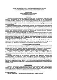
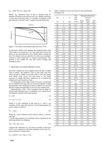
S ult = (0.08 *D+3.8) + (Q ultL/AE) (1)
Where: S ult: settlement (mm) of pile at ultimate load, D:
diameter of the pile at the pile tip (cm), Qult: ultimate load (ton),
A: base area of the pile (mm 2 ), E: modulus of elasticity of the
pile material (2 ton/mm 2 ) and L: length of the pile shaft (mm).
Settlement, S
0 50 100 150 200 250
Qult
300 350
0
O
2
4
6
8 C
10
12
14
16
18
20
Figure 1. The Offset Limit Method (after Davisson 1972).
In Davisson’s Offset Limit Method, the predicted failure load
value tends to be conservative [3]. The actual limit line can be
drawn on the load-settlement curve already before starting the
test. The ultimate load can, therefore, be used as an acceptance
criterion to proof tested piles in contract specifications. This
method is not suitable for tests that involve loading and
unloading cycles.
3 PROPOSED DAVISSON MODIFICATION
Davisson’s method can not be applied unless the pile is loaded
close to failure. The problem is that in most static load tests
where the pile is loaded to one and a half or twice the design
load, failure rarely occurs. For this reason it was found
necessary to modify Davisson’s method so as to estimate the
ultimate pile load from the test load.
For the purpose of this study, results of seventy six axial load
tests on different pile types (driven, bored and augered), lengths
and diameters were considered as shown in table (1) for one and
half the working load and table (2) for twice the working load.
Brinch-Hansen, (1961, 1963) considered that the shape of
the pile load-settlement curve is a parabolic curve which can be
calculated by using the following equation:
S = a Q 2
(2)
a = 1/ (C 1 S + C 2) 2
Where S is pile settlement at pile load Q, C 1 and C 2 are
constants, for the same pile load test. At test load equation (2)
can be written as follows:
STL = a Q TL 2
Where S TL is pile settlement at pile load test, and Q TL is the test
pile load.
By dividing equation (2) at ultimate load by equation (4) the
following relation was obtained:
Qult 2 = Q TL 2 [Sult / S TL] (5)
Ultimate pile settlement, Sult, was taken according to Davisson
(1972), as in equation (1) and pile settlement at test load, STL,
can be written in a similar form:
S TL= (0.08 D+ 3.8) + (Q TL L /A E) (6)
2080
Load, Q
QL/AE O1
C1
(3)
(4)
Table 1: Results of Axial Load Tests for One and Half the
Working Load
Test L D
Test
load
(ton)
No m mm 1.5 W.L Elastic
Sett.
Measured settlement at
Test Load
(mm)
Plastic
Sett.
Total
Sett..
Dr1 13 450 67.5 1.85 0.38 2.23
Dr2 17.5 500 67.5 4.00 0.41 4.40
Dr3 14.75 530 120 2.43 0.33 2.75
Dr4 22.25 430 75 2.68 0.12 2.80
Dr5 19.3 400 60 2.18 1.62 3.80
Dr6 15 400 60 1.98 0.40 2.38
Dr7 26.5 600 195 4.37 0.67 5.04
Dr8 13 400 80 2.98 1.30 4.28
B9 22.85 800 262.5 0.94 1.13 2.06
B10 13.1 500 105 2.09 1.19 3.27
B11 11 500 75 1.02 0.97 1.99
B12 12 500 85 1.59 2.57 4.16
B13 14.55 600 90 0.49 0.26 0.75
B14 13.35 450 52.5 0.62 0.32 0.94
B15 13.5 800 187.5 1.48 4.25 5.73
B16 17.25 600 150 2.19 2.37 4.56
B17 12.5 800 240 2.62 7.78 10.40
B18 13 600 153.75 5.23 5.04 10.27
B19 22.5 600 120 0.90 0.58 1.48
B20 21 600 75 1.15 0.33 1.48
B21 14.8 400 45 1.21 0.20 1.41
B22 20 600 150 0.96 1.63 2.58
B23 20 600 157.5 2.45 1.56 4.01
B24 13.35 450 52.5 0.56 0.32 0.88
F25 18 650 210 2.48 1.33 3.81
F26 18 600 180 2.95 1.29 4.24
F27 18 600 180 3.22 1.65 4.87
F28 14 600 120 1.33 0.75 2.08
F29 14 600 120 1.24 0.28 1.52
F30 14 600 120 0.99 0.66 1.65
F31 13.6 400 45 1.78 2.22 4
F32 13.6 400 45 1.22 1.65 2.87
F33 12 600 90 0.63 0.54 1.17
F34 13.2 400 30 0.48 0.26 0.74
F35 12.2 400 30 0.46 0.23 0.69
F36 12.2 400 30 0.49 0.26 0.75
F37 15 400 30 0.41 0.21 0.62
F38 12.2 400 30 0.35 0.37 0.72
F39 21 500 97.5 0.79 0.57 1.36
F40 21 500 97.5 1.77 0.57 2.34
F41 15 600 150 2.95 3.3 6.25
F42 25 400 55.5 0.81 0.37 1.18