Modification of Davisson's method

Modification of Davisson’s method
Modification de la methode de Davisson
F.A. Baligh
Faculty of Engineering, Helwan University
G.E. Abdelrahman
Faculty of Engineering, Cairo University-Fayoum Branch
ABSTRACT
Davisson’s method (Offset Limit Method) is probably the best-known and most widely used method for predicting the ultimate pile
load from load test results. This method when applied to the load-settlement curve of a tested pile, usually fails, unless the pile is
loaded close to failure. Results of eighty static axial load tests on different types of piles carried out in Egypt were analyzed according
to Davisson’s method to obtain the ultimate load. Only four out of the eighty tests satisfied the method and predicted the ultimate
load.
Elastic and plastic settlements were measured for each pile load test at test load. These values were compared with those obtained
from their relevant parts in Davisson’s equation. Davisson’s equation, when applied at test load equal to either one and a half or twice
the working load, gives values higher than those measured for both the elastic and plastic parts.
Davisson’s equation was modified to accommodate the difference between the calculated and the measured values at the test load.
The suggested form of Davisson’s equation allows the prediction of the pile ultimate load using the pile test load without having to
extrapolate the load-settlement curve.
RÉSUMÉ
La méthode de Davisson une des plus propagé méthode pour prédire le poids le plus grand charge ultime pour les pieux et cette
méthode quand elle faite sur le courbe du poids et la rupture du pieu examiné toujours ne reussi pas sauf si que le pieu se met presque
au poids détructeur. Les résultats de 80 expériences pour les poids verticales sur plusieurs genres des pieux ont étaient faite en Egypte
et elles étaient calculées par la méthode du Davisson pour produire la charge ultime du poids du pieu , il’ya4 expériences seulement
des 80 expériences satisfées la méthode et la prédiction de la charge ultime.
Le tassement de l’élastic et le plastic sont mesurés pour chaque expérience a une poids expériencelle . Ces valeurs sont compares avec
ceux qui sont calcules de la équation de Davisson . L’équation de Davisson quand elle applique au poids expériencelle une fois et
demi ou deux fois donne des résultats plus grand que les mesures de l’expérience de l’élastic et le plastic.
L’équation de Davisson était modifiée pour accommoder le difference entre la valeur qui était calculée et la valeur qui était mesurée
au poids expériencelle. La forme proposé du méthode de Davisson permit la prédiction du charge la plus grand ultime pour le pieu
par utiliser le poids experiencelle a l’allongement du poids et du tassement du pieu .
1 INTRODUCTION
The working load or design load is the load a pile is designed to
carry safely within a limited range of settlement; this limited
settlement range depends on the nature of the building, its
importance and also the properties of soil in which the pile is
installed. Design load is pre-calculated using field and
laboratory test results. Load tests are performed to prove the
design load and check the pre-chosen factor of safety.
A method to insure the above was proposed by Davisson
(1972); which is easy to apply and has gained wide acceptance.
The Offset Method defines failure as the intersection of the
elastic stiffness of the pile drawn through an offset on the
abscissa that depends on the pile diameter. Since the offset is
defined by the pile diameter, the capacity is dependent on the
pile diameter.
The proposed modified method estimates the ultimate pile
load from the axial pile load test by using a reduction factor for
Davisson equation. For the purpose of this study, results of
seventy six field axial load tests database on different pile types
were compiled. The tested piles included driven, bored, and
continuous flight auger piles with different diameters. The tests
were carried out at various locations in different Egyptian soils.
The soils for all the sites consisted of different layers of silty clay
to fine sand along the pile length and the pile tip ended in medium
to graded sand.
2 THE DAVISSON OFFSET LIMIT LOAD
The method was proposed by Davisson (1972) as the load
corresponding to the movement that exceeds the elastic
compression of the pile (taken as a free standing column) by a
value of 3.8 mm plus a factor equal to the diameter of the pile
(in cm) divided by 10.
The method is based on the assumption that ultimate
capacity is reached at a certain small toe movement. It was
primarily intended for test results from driven piles, but when
applied to bored piles, it becomes impractically conservative.
The offset limit criterion is intended for interpretation of quick
testing, in which each load increment is held for periods not
exceeding one hour. It can also be used when interpreting
results from slow methods. This method also gained widespread
use in phase with the increasing popularity of wave equation
analysis of driven piles and dynamic testing.
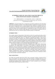
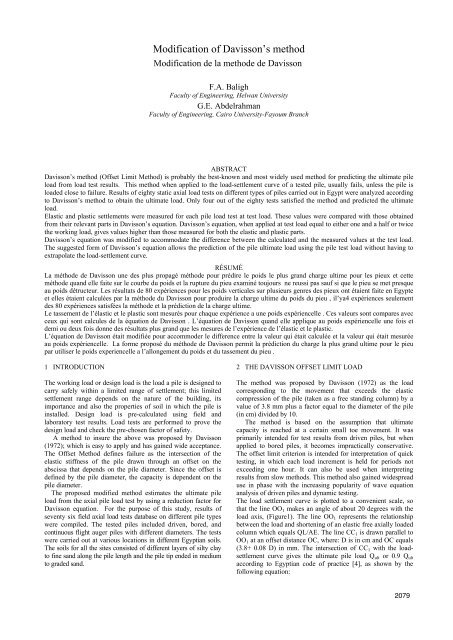
The load settlement curve is plotted to a convenient scale, so
that the line OO1 makes an angle of about 20 degrees with the
load axis, (Figure1). The line OO 1 represents the relationship
between the load and shortening of an elastic free axially loaded
column which equals QL/AE. The line CC1 is drawn parallel to
OO1 at an offset distance OC, where: D is in cm and OC equals
(3.8+ 0.08 D) in mm. The intersection of CC1 with the loadsettlement
curve gives the ultimate pile load Q ult or 0.9 Q ult
according to Egyptian code of practice [4], as shown by the
following equation:
2079

S ult = (0.08 *D+3.8) + (Q ultL/AE) (1)
Where: S ult: settlement (mm) of pile at ultimate load, D:
diameter of the pile at the pile tip (cm), Qult: ultimate load (ton),
A: base area of the pile (mm 2 ), E: modulus of elasticity of the
pile material (2 ton/mm 2 ) and L: length of the pile shaft (mm).
Settlement, S
0 50 100 150 200 250
Qult
300 350
0
O
2
4
6
8 C
10
12
14
16
18
20
Figure 1. The Offset Limit Method (after Davisson 1972).
In Davisson’s Offset Limit Method, the predicted failure load
value tends to be conservative [3]. The actual limit line can be
drawn on the load-settlement curve already before starting the
test. The ultimate load can, therefore, be used as an acceptance
criterion to proof tested piles in contract specifications. This
method is not suitable for tests that involve loading and
unloading cycles.
3 PROPOSED DAVISSON MODIFICATION
Davisson’s method can not be applied unless the pile is loaded
close to failure. The problem is that in most static load tests
where the pile is loaded to one and a half or twice the design
load, failure rarely occurs. For this reason it was found
necessary to modify Davisson’s method so as to estimate the
ultimate pile load from the test load.
For the purpose of this study, results of seventy six axial load
tests on different pile types (driven, bored and augered), lengths
and diameters were considered as shown in table (1) for one and
half the working load and table (2) for twice the working load.
Brinch-Hansen, (1961, 1963) considered that the shape of
the pile load-settlement curve is a parabolic curve which can be
calculated by using the following equation:
S = a Q 2
(2)
a = 1/ (C 1 S + C 2) 2
Where S is pile settlement at pile load Q, C 1 and C 2 are
constants, for the same pile load test. At test load equation (2)
can be written as follows:
STL = a Q TL 2
Where S TL is pile settlement at pile load test, and Q TL is the test
pile load.
By dividing equation (2) at ultimate load by equation (4) the
following relation was obtained:
Qult 2 = Q TL 2 [Sult / S TL] (5)
Ultimate pile settlement, Sult, was taken according to Davisson
(1972), as in equation (1) and pile settlement at test load, STL,
can be written in a similar form:
S TL= (0.08 D+ 3.8) + (Q TL L /A E) (6)
2080
Load, Q
QL/AE O1
C1
(3)
(4)
Table 1: Results of Axial Load Tests for One and Half the
Working Load
Test L D
Test
load
(ton)
No m mm 1.5 W.L Elastic
Sett.
Measured settlement at
Test Load
(mm)
Plastic
Sett.
Total
Sett..
Dr1 13 450 67.5 1.85 0.38 2.23
Dr2 17.5 500 67.5 4.00 0.41 4.40
Dr3 14.75 530 120 2.43 0.33 2.75
Dr4 22.25 430 75 2.68 0.12 2.80
Dr5 19.3 400 60 2.18 1.62 3.80
Dr6 15 400 60 1.98 0.40 2.38
Dr7 26.5 600 195 4.37 0.67 5.04
Dr8 13 400 80 2.98 1.30 4.28
B9 22.85 800 262.5 0.94 1.13 2.06
B10 13.1 500 105 2.09 1.19 3.27
B11 11 500 75 1.02 0.97 1.99
B12 12 500 85 1.59 2.57 4.16
B13 14.55 600 90 0.49 0.26 0.75
B14 13.35 450 52.5 0.62 0.32 0.94
B15 13.5 800 187.5 1.48 4.25 5.73
B16 17.25 600 150 2.19 2.37 4.56
B17 12.5 800 240 2.62 7.78 10.40
B18 13 600 153.75 5.23 5.04 10.27
B19 22.5 600 120 0.90 0.58 1.48
B20 21 600 75 1.15 0.33 1.48
B21 14.8 400 45 1.21 0.20 1.41
B22 20 600 150 0.96 1.63 2.58
B23 20 600 157.5 2.45 1.56 4.01
B24 13.35 450 52.5 0.56 0.32 0.88
F25 18 650 210 2.48 1.33 3.81
F26 18 600 180 2.95 1.29 4.24
F27 18 600 180 3.22 1.65 4.87
F28 14 600 120 1.33 0.75 2.08
F29 14 600 120 1.24 0.28 1.52
F30 14 600 120 0.99 0.66 1.65
F31 13.6 400 45 1.78 2.22 4
F32 13.6 400 45 1.22 1.65 2.87
F33 12 600 90 0.63 0.54 1.17
F34 13.2 400 30 0.48 0.26 0.74
F35 12.2 400 30 0.46 0.23 0.69
F36 12.2 400 30 0.49 0.26 0.75
F37 15 400 30 0.41 0.21 0.62
F38 12.2 400 30 0.35 0.37 0.72
F39 21 500 97.5 0.79 0.57 1.36
F40 21 500 97.5 1.77 0.57 2.34
F41 15 600 150 2.95 3.3 6.25
F42 25 400 55.5 0.81 0.37 1.18

Table 2: Results of Axial Load Tests for Twice the Working
Load
Test L D
Test
load
(ton)
No m mm 2 W.L
Measured settlement at
Test Load
Elastic
Sett.
(mm)
Plastic
Sett.
Total
Sett.
Dr1 23 500 120 1.79 0.55 2.33
Dr2 17 430 80 2.65 0.79 3.44
Dr3 13.6 500 95 2.00 0.56 2.56
Dr4 20 400 50 2.30 0.59 2.89
Dr5 26 450 90 2.26 1.65 3.91
Dr6 19.7 400 60 1.30 0.12 1.41
Dr7 11.75 400 70 0.92 0.71 1.63
Dr8 23.75 400 70 2.82 0.29 3.11
Dr9 12 500 34 0.91 0.36 1.26
Dr10 14.75 400 70 1.68 0.63 2.31
Dr11 17.2 400 128 1.17 0.39 1.56
Dr12 19.5 400 80 5.27 2.30 7.57
Dr13 12 400 80 1.16 0.25 1.41
Dr14 19.5 450 50 0.49 0.09 0.58
Dr15 23.5 450 90 3.06 1.20 4.26
B16 25.2 800 350 2.72 2.27 4.99
B17 13.5 500 120 2.16 4.10 6.26
B18 14 600 130 2.68 2.82 5.50
B19 14 600 130 2.57 3.10 5.67
B20 15.5 600 120 3.21 1.49 4.70
B21 17.5 800 350 8.65 5.74 14.39
B22 12.8 800 350 5.88 9.30 15.18
B23 17 800 120 6.65 10.74 17.39
B24 18 800 340 6.35 5.27 11.62
B25 20 800 350 3.55 1.81 5.36
B26 16.5 600 147 1.67 2.155 3.82
F27 19.6 600 210 3.27 0.42 3.69
F28 19.6 600 210 2.10 0.47 2.57
F29 19.6 600 210 4.14 0.905 5.047
F30 19.6 600 210 3.46 6.15 9.61
F31 19.6 600 210 2.09 0.52 2.61
F32 19.6 600 210 3.34 0.24 3.58
F33 19.6 600 210 3.38 0.22 3.6
F34 13.6 400 60 0.81 1.1 1.91
Dr: driven pile cast in situ.
B: bored pile.
F: continuous flight augered pile.
L: pile length.
D: pile diameter.
Comparing separately the two terms of equation (6) at test load
to the measured plastic and elastic settlement at test load, the
results are shown in Figures (2 to 5). It can be seen that the
plastic part presented in Figure (2) and the elastic part presented
in Figure (3) for test load at one and half the working load, and
similarly in Figures (4) and (5) for the case where the test load
is twice the working load, equation (6) over estimates the plastic
and elastic pile behavior. In order to predict the modified
Davisson’s equation using pile test load, QT.L, in case of the test
load one and half, and twice the working load, the following
equations were suggested respectively:
STL= (0.06 D – 1.9) + 0.5 (Q T.LL/EA) (mm) (7)
S TL= (0.12 D – 4) + 0.85 ((Q T.LL/EA) -2) (mm) (8)
Where: D = pile diameter (cm), Q T.L= pile load test at one and
half the working load (ton) L = pile length (mm), E = pile
Young’s modulus (2 ton/mm 2 ), and A = pile cross section area
(mm 2 ).
By substituting in equation (5) in case the test load is one
and half the working load the ultimate pile load Q ult may be
calculated using pile test load, Q TL, as follows:
Q
2
ult
Q
2
TL
Qult
L
[ 0.
08D
+ 3.
8]
+
EA
QTL
L
[ 0.
06D
−1.
9]
+
2EA
= (9)
Similarly, if the test load is twice the working load the ultimate
pile load Qult may be calculated using pile test load, Q TL, as
follows:
Q
2
ult
Pile Settlem ent S m m
= Q
2
Qult
L
[ 0.
08D
+ 3.
8]
+
EA
QTL
L
[ 0.
12D
− 4]
+ 0.
85[
− 2]
EA
TL (10)
Comparisson Between Suggested, Measured, and Davisson
Plastic Behavior
15
Measured
12
Suggested
9
6
3
0
0 100 200 300 400
Test Load Q ton
Davisson
Measured trendline
Suggested trendline
Davisson trendline
Figure 2. Plastic behavior for test load one and half the working
load.
2081

Pile Settlement mm
Comparisson Between Suggested, Meassured, and Davisson
Elastic Behavior
15
12
9
6
3
0
0 100 200 300 400
Test Load Q ton
Suggested
Measured
Davisson
Suggested trendline
Measured trendline
Davisson trendline
Figure 3. Elastic behavior for test load one and half the working
load.
Pile Settlement S mm
15
12
9
6
3
0
Comparisson Between Suggested, Measured, and Davisson Plastic
Behavior
0 100 200 300 400
Test Load Q ton
Measured
Suggested
Davison
Suggested trendline
Davisson trendline
Measured trendline
Figure 4. Plastic behavior for test load twice the working load.
Pile Settlem ent S m m
Comparison Between Suggested, Measured, and Davisson Elastic
Behavior �
15
12
9
6
3
0
0 100 200 300 400
Test Load Q ton
Suggested
Measured
Davisson
Suggested trendline
Measured trendline
Davisson trendline
Figure 5. Elastic behavior for test loads twice the working load.
A comparison was carried out between measured and suggested
elastic and plastic pile settlements as shown in Figure (6) in
case the test load is one and half the working load and Figure
(7) in case the test load is twice the working load.
4 SUMMARY AND CONCLUSIONS
Davisson’s method needs the pile to be loaded near to failure
to be applicable. Davisson’s equation when applied for test
load it highly over estimated the elastic and plastic settlements.
The suggested form of Davisson’s equation allows the
prediction of the pile ultimate load using the pile test load
without having to extrapolate the load-settlement curve. Since
equations (9 and 10) are equations of the second degree in Qult
they can be easily solved to obtain the ultimate pile load.
2082
Suggested Settlement. mm
Comparisson Between Suggested and Measured Elastic
Settlement
10
8
6
4
2
0
elastic settlement
Plastic settlement
0 2 4 6 8 10
Measured Settlement mm
Figure 6. Measured and suggested elastic and plastic pile
settlement in case the test load is one and half the working load.
Suggested Settlement. mm
10
8
6
4
2
0
Comparisson Between Suggested and Measured Elastic
Settlement
Elastic settlement
Plastic settlement
0 2 4 6 8 10
Measured Settlement mm
Figure 7. Measured and suggested elastic and plastic pile
settlement in case the test load is twice the working load.
REFERENCES
Canadian Geotechnical Society, 1992. Canadian Foundation
Engineering Manual.
Davisson, M.T. 1970. Design Pile Capacity. Proc., Conf. on Design and
Installation of Pile Foundations and Cellular Structures, Lehigh
Univ., Envo Public. Co. pp. 75-85.
Davisson, M.T. 1972. High Capacity Piles. Proceedings, Lecture Series,
Innovations in Foundation Construction, ASCE, Illinois Section,
Chicago, March 22, pp. 81-112.
Egyptian Code of Soil Mechanics and Foundation Engineering, 1995.
Part 4.