Yamada and Matsumoto Shift Right Left

Yamada and Matsumoto
3 Deterministic Dependency Analysis
3.1
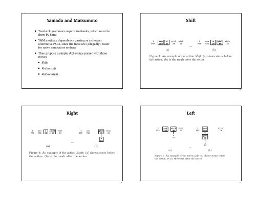
• Treebank grammars require treebanks, which must be
Three parsing draw actions by hand
target nodes, and the point of focus simply moves to the right. Figure 3 shows an example of a
Shift action. The result of Shift in Figure 3(b) shows that target nodes move to the right, i.e.,
from “saw” and “a” to “a” and “girl”.
Our parser constructs • Y&M dependency motivate trees dependency in left-to-right parsing word as a order cheaper of input sentences based on
three parsing actions: alternative Shift, RightPSGs, and Left. since These the trees actions are (allegedly) can be applicable easier to two neighboring
for naive annotators to draw
words (referred to as target nodes). Shift means no construction of dependencies between these
target nodes, and the • They pointpropose of focusa simply simple moves shift-reduce to the parser right. Figure with three 3 shows an example of a
moves
Shift action. The result of Shift in Figure 3(b) shows that target nodes move to the right, i.e.,
from “saw” and “a” to • “a” Shift and “girl”.
I saw a girl with
I saw a girl with
PRP VBD DT NN IN
PRP VBD DT NN IN
→
(a) (b)
Figure 3: An example of the action Shift: (a) shows states before
the action. (b) is the result after the action
I
PRP
• Reduce Left
saw a girl with
VBD DT NN IN
• Reduce Right
(a)
→
I
PRP
saw
VBD
a
DT
(b)
girl
NN
with
IN
A Right action constructs a dependency relation between two neighboring words where the
left node of target nodes becomes a child of the right one. Figure 4 is an example of the action
Right. After applying this action, “a” becomes a child of “girl” (“a” modifies “girl”). We
Figure 3: An example of the action Shift: (a) shows states before
the action. (b) is the result after the action
A Right action constructs a dependency relation between two neighboring words where the
left node of target nodes becomes a child of the right one. Figure 4 is an example of the action
Right. After applying this action, “a” becomes a child of “girl” (“a” modifies “girl”). We
Right
should point out that the next target nodes are “saw” and “girl” after executing the action in
our current algorithm, keeping the right frontier focus point unchanged.
I
PRP
saw
VBD
a
DT
girl
NN
with
IN
I
PRP
saw
VBD
→
(a) (b)
girl
NN
a
DT
with
IN
Figure 4: An example of the action Right: (a) shows states before
the action. (b) is the result after the action
1
3 Deterministic Dependency Analysis
3.1 Three parsing actions
Our parser constructs dependency trees in left-to-right word order of input sentences based on
three parsing actions: Shift, Right and Left. These actions can be applicable to two neighboring
Shift
words (referred to as target nodes). Shift means no construction of dependencies between these
should point out that the next target nodes are “saw” and “girl” after executing the action in
our current algorithm, keeping the right frontier focus point unchanged.
I
PRP
saw
VBD
a
DT
girl
NN
with
IN
I
PRP
saw
VBD
→
(a) Left
(b)
girl
NN
a
DT
with
IN
Figure 4: An example of the action Right: (a) shows states before
the action. (b) is the result after the action
Note that when Figure either5: ofAn Left example or Right of theaction action is Left: applicable (a) shows the states dependent before child, the child
should be a complete the subtree action. (b) tois which the result no further after thedependent action children will exist. For the parser
to guarantee this, we have to make the parser to be able to see the surrounding context of the
target nodes. This will be seen in the next section.
The Left action constructs a dependency relation between two neighboring words where the dependency tree by executing the estimated actions. Figure 6 shows the pseudo-code of our
right node of target nodes becomes a child of the left one, opposite to the action Right. Figure 3.2 parsing Parsing algorithm. Algorithm
5 shows an example of the Left action.
Our parsing algorithm consists of two procedure: (i) Estimation of appropriate parsing actions
3
4
Input Sentence: (w1, p1), (w2, p2), · · · , (wn, pn)
using contextual information Initialize: surrounding the target nodes, and (ii) the parser constructs a
Note that when either of Left or Right action is applicable the dependent child, the child
i = 1 ;
should be a complete subtree to which no further dependent children will exist. For the parser
T = {(w1, p1), (w2, p2), · · · , (wn, pn)}
no construction = true ;
I
PRP
saw
VBD
girl
NN
with
IN
a
girl
The Left action constructs a dependency DT relation between NN two neighboring words where the
right node of target nodes becomes a child of the left one, opposite to the action Right. Figure
a
5 shows an example of the Left action.
→
DT
(a) (b)
I
PRP
saw
VBD
with
IN
2

Parsing algorithm
• start at the left edge of the sentence
• Shift, Left, or Right
• repeat until either:
• the window has Shifted to the right edge
• if we had at least one reduction during the last
pass through the sentence, then start again at the
left edge
• otherwise, FAIL
• there’s only one unreduced word left
• SUCCEED
Decision trees
Outlook?
sunny overcast rain
Humidity?
Yes
high normal
No Yes
strong
No
Wind?
weak
Yes
5
7
Parsing algorithm
• All we need is some way of choosing a parser action
• Predicting the next move is a classification problem:
assign one or more labels L from a finite set to
instances I
• Classification problems come up frequently in NLP, and
can be approached probabilistically by using a model to
estimate P(I, L)
• Classifiers can also be built by hand, e.g., as a cascade
of finite state transducers which map from I to L
• A wide range of NLP tasks can be cast as classification
problems
Decision trees
• Decision trees are well suited to represent problems
where instances are vectors of discrete-valued features
and the target function has predefined discrete values
• Value of target function is a ‘logical’ combination of
feature values (no weights, logs, sums, etc.)
• NLP classification problems very often look like this
• If necessary, continuous (interval) variables can be
converted to discrete (ordinal or nominal) variables
(discretization)
6
8

Decision trees
• Decision trees can be constructed manually by a
knowledge engineer
• It’s more fun to induce a decision tree from a collection
of labeled instances
• Early work on Divide and conquer algorithms:
Hoveland, Hunt (1950’s and 60’s)
• Friedman, Breiman = CART (1984)
• Algorithms ID3 and C4.5 (and others) developed by
Ross Quinlan (1978—now)
Overfitting
• Like all learning algorithms, ID3 sometimes suffers
from overfitting (aka overtraining):
Given a hypothesis space H, a hypothesis h is said to
overfit the training data is there exists some alternative
hypothesis h!, such that h has a smaller error than h!
over the training examples, but h! has a smaller error
than h over the entire distribution of instances.
• Overfitting is particular worrisome for models which
are not well specified, or for sparse, noisy, nondeterministic
data (sound familiar?)
9
11
Accuracy
0.9
0.85
0.8
0.75
0.7
0.65
0.6
0.55
Decision trees
• Day Outlook Temp Humid Wind Play?
d1 sunny hot high weak no
d2 sunny hot high strong no
d3 overcast hot high weak yes
d4 rain mild high weak yes
d5 rain cool normal weak yes
d6 rain cool normal strong no
d7 overcast cool normal strong yes
d8 sunny mild high weak no
d9 sunny cool normal weak yes
d10 rain mild normal weak yes
d11 sunny mild normal strong yes
d12 overcast mild high strong yes
d13 overcast hot normal weak yes
d14 rain mild high strong no
Overfitting
0.5
0 10 20 30 40 50 60 70 80 90 100
Size of tree (number of nodes)
On training data
On test data
10
12

Support Vector Machines
• Instead of decision trees, Y&M use Support Vector
Machines (SVMs), a state-of-the-art classification
algorithm
• Based on Vapnik’s statistical learning theory
Margin
Positive Example
Negative Example
w x + b > 1
w x + b = 0
w x + b < -1
Positive Support Vector
Negative Support Vector
Figure 2: Overview of Support Vector Machine
non-separable case (see [11, 12] for the details). Finally, the optimal hyperplane is written as
follows.
Features
�
l�
�
• To apply f(x) SVMs, = sign we need αiyiK(xi, some way x) + of b representing
parser contexts i
where αi is the Lagrange multiplier corresponding to each constraint, and K(x ′ , x ′′ Context
) is called a
kernel function, it calculates similarity between two arguments x ′ and x ′′ left context target nodes right context . SVMs estimate the
label of an unknown example x whether sign of f(x) is positive or not.
floor
NN
--
:
sellers
NNS
of
IN
resort
NN
There are two advantages in using SVMs for statistical dependency analysis: (i) High gen-
eralization performance in high dimensional feature werespaces.
SVMs optimize the pa-
the
DT
rameter w and b of the separate hyperplane based on maximum margin strategy. This strategy
guarantees theoretically the low generalization error for an unknown example in high dimen-
use of these node as features
VBN
sional feature space [12]. (ii) Learning with combination of multiple features is possible
by virtue of polynomial kernel functions. SVMs can deal with non-linear classification
using kernel functions. Especially use of the polynomial function (x ′ · x ′′ + 1) d as the kernel,
Figure 7: An example of contextual information
such an optimal hyperplane has an effect of taking account of combination of d features without
causing a large amount of computational cost. Owing to these advantages, we can train rules of
15
the learned SVMs.
dependency structure analysis using many features including not only part-of-speech tags and
The role of the variable no construction is to check whether there have been any actions
word itself, but also their combination.
to construct of dependencies at the end of the sentence. The value being true means that the
SVMs model arehas discriminative estimated Shift classifiers, actions to and all the not target generative nodes (from probabilistic i = 1 to i = models |T |) inlike the naive parsingBayes
last
JJ
who
WP
VBD
criticized
-- once --
: RB :
13
(2)
Support Vector Machines
• SVMs are two-class classifiers: they divide the data into
a positive and negative regions
• SVMs are non-parametric, discriminate classifiers
• no joint probability model
• no probability model at all
• For choosing parser actions, Y&M build three SVMs
• Reduce Left vs. Reduce Right
• Reduce Left vs. Shift
• Reduce Right vs. Shift
• Majority wins
Features
denotes those in the right context. The feature type k and its value v are summarized in Table
1. In Table 1, ch-L-pos, ch-L-lex, ch-R-pos and ch-R-lex are information of child nodes within
• The context size determines how far to the left or right
we can look
• The feature set determines what aspects of the context
get encoded in an instance
the context, and are called as child features. In the analysis of prepositions, auxiliary verbs,
or relative pronouns, the information about their children would be a good preference whether
dependencies are constructed or not. In Figure 7, “were”, is one of the child features of “who”,
predicates that “who” modifies to plural noun “sellers”, not modifies singular noun “resort”.
Child features are dynamically determined in the step of analysis.
Table 1: Summary of the feature types and their values.
type value
pos part of speech(POS) tag string
lex word string
ch-L-pos POS tag string of the child node modifying to the parent node from left side
ch-L-lex word string of the child node node modifying to the parent node from left side
ch-R-pos POS tag string of the child node modifying to the parent node from right side
ch-R-lex word string of the child node modifying to the parent node from right side
For example, in Figure 7, the features are as follows: (-2, pos, :), (-2, lex, –), (-1, pos, NNS),
(-1, lex, sellers), (-1, ch-R-pos, DT), (-1, ch-R-lex, the), (0-, pos, IN), (0-, lex, IN), (0+, pos,
NN), (0+, lex, resort), (0+, ch-R-pos, JJ), (0+, ch-R-lex, last), (+1, pos, WP),( +1, lex, who),
(+1, ch-L-pos, VBD), (+1, ch-L-lex, were), (+2, pos, :), (+2, lex, –).
4.2 Grouping training example for reducing learning cost
The computational cost for training SVMs is roughly proportional to l 2 or l 3 (l is the number
14
16

Firstly “curse we of investigate dimensionality”, the performance since the number and degrees of dimension of polynomial of feature kernel spaces taking functions. account Table of 2
illustrates the combination the dependency of more than accuracy threefor features the different is much larger number thanofindegrees d = 2. of polynomial kernel
functions. The best result is obtained at d = 2. However, all of the results in d ≥ 2 are
superior to that of d = 1. The results suggest that in the learning of dependency structure
Table 2: Dependency accuracies and degrees of polynomial kernel functions:
it requires to Context take account length is of (2,2). combination Use of all features of multiple described features, in Table not solely 1. with single features.
The accuracy of d = 3 and d = 4 are lower than d = 2. It may be overfitting by the well known
d : (x
“curse of dimensionality”, since the number Results of dimension of feature spaces taking account of
the combination of more than three features is much larger than in d = 2.
′ · x ′′ + 1) d
1 2 3 4
Dep. Acc. 0.854 0.900 0.897 0.886
Root Acc. 0.811 0.896 0.894 0.875
Comp. Rate 0.261 0.379 0.368 0.346
Table 2: Dependency accuracies and degrees of polynomial kernel functions:
We investigate Context length the performance is (2,2). Useand of all thefeatures differentdescribed length of in context. Table 1. Table 3 illustrates the
d : (x ′ · x ′′ + 1) d
results of each length of context. The best of dependency accuracy and root accuracy is at the
model (2, 4), and (3, 3) is the best result1of complete 2 rate. 3This demonstrates 4 that the dependency
accuracy dependsDep. on theAcc. context0.854 length, and 0.900 the longer 0.897the0.886 right context contributes the
performance. The resultRoot of (2,5) Acc. was worse 0.811than0.896 that of (2,4). 0.894One 0.875 reason behind this lies that
features which are notComp. effectiveRate for parsing 0.261are included 0.379 in 0.368 the context 0.346(2,5).
We investigate the performance and the different length of context. Table 3 illustrates the
Table 3: Dependency accuracies and the length of context: Kernel function is (x
results of each length of context. The best of dependency accuracy and root accuracy is at the
′ ·
x ′′ + 1) 2 . Use of all features described in Table 1.
model (2, 4), and (3, 3) is the best result of complete rate. This demonstrates that the depen-
(l, r): context length
dency accuracy depends on (2, the 2) context (2, 3) length, (2, 4) and (2, the 5) longer (3, 2) the (3, right 3) context (3, 4) contributes (3,5) the
performance. Dep. TheAcc. result 0.900 of (2,5) 0.903 was worse 0.903 than 0.901 that of (2,4). 0.898 One 0.902 reason 0.900 behind 0.897 this lies that
Root Acc. 0.896 0.911 0.916 0.913 0.897 0.915 0.912 0.909
features which are not effective for parsing are included in the context (2,5).
Comp. Rate 0.379 0.382 0.384 0.375 0.373 0.387 0.373 0.366
Table 3: Dependency accuracies and the length of context: Kernel function is (x ′ ·
x ′′ + 1) 2 Next, we investigate which features contribute the dependency accuracy, especially focusing
. Use of all features described in Table 1.
(l, r): context length
(2, 2) (2, 3) (2, 4) (2, 5) (3, 2) (3, 3) (3, 4) (3,5)
Dep. Acc. 0.900 0.903 0.903 0.901 0.898 0.902 0.900 0.897
Root Acc. 0.896 0.911 0.916 0.913 0.897 0.915 0.912 0.909
Comp. Rate 0.379 0.382 0.384 0.375 0.373 0.387 0.373 0.366
Next, we investigate which features contribute the dependency accuracy, especially focusing
Results
Table 5: Comparison with related work.
Charniak Collins Our parser
model 1 model 2 model 3
Dep. Acc. 0.921 0.912 0.915 0.915 0.903
Root Acc. 0.952 0.950 0.951 0.952 0.916
Comp. Rate 0.452 0.406 0.431 0.433 0.384
Leaf Acc. 0.943 0.936 0.936 0.937 0.935
corresponding to base noun phrase, the dependency tree would be able to predicate that the
subtree is a part of the noun phrase according to the parent nodes and each part of speech
tag. In fact, Leaf Acc. of our parser, which denotes the dependency accuracy of leaf nodes, is
comparable to Collins’ in Table 5. 2
In the analysis nearby root of the dependency trees, the phrase structure parsers can use
richer information than our parser. Our parser estimates dependency relation between19the top nodes of subtrees which corresponds to the clause of sentence, or verb phrase including
the head of the sentence. The structure of these subtrees is similar to each other, i.e., the
parent node is verb and the children consist of nouns, prepositions, or adverbs. Therefore it
17
Results
on the child features. We examine the following five sets of features:
(a) No use of child features (only pos and lex in Table 1)
(b) Use of only lexical features of child nodes (pos, lex, ch-L-lex and ch-R-lex in Table 1)
(c) Use of only part of speech(POS) tag features of child node (pos, lex, ch-L-pos and
ch-R-pos in Table 1)
(d) If POS tag of the parent node is IN, MD, TO, WP or WP$, and the POS tag of the
child is NN, NNS, NNP, NNPS, VB, VBD,VBG, VBN, VBP, VBZ, IN, or MD, then
using of POS tag and lexical feature of child nodes, otherwise only POS tag features of
child.
(e) Use of both POS tag and lexical features of child nodes (All of features in Table 1)
Table 4: Dependency accuracies and five sets of features: (Context
length is (2,4). Kernel function is (x ′ · x ′′ + 1) 2 .)
(a) (b) (c) (d) (e)
Dep. Acc. 0.890 0.901 0.902 0.902 0.903
Root Acc. 0.882 0.915 0.912 0.913 0.916
Comp. Rate 0.348 0.383 0.374 0.377 0.384
num. of features 290,008 441,842 290,362 323,262 442,196
Table 4 shows the results of each feature set. The accuracy of (a) is lower than all others. The
result shows that dynamic use of dependencies estimated by SVMs is effective for the following
18
parsing process even in deterministic manner. The best result is (e) and comparable to the
result of (b). The accuracy of (e) and (b) are superior to (c) and (d) even though feature set (e)
and (b) include all of the lexical information appeared in the training examples and are much
more higher dimensional feature space than both feature set (c) and (d). The results suggest
that the lexical information is more effective features for dependency analysis.
Conclusions
5.2 Comparison with Related Work
We compare our parser with other statistical parsers: maximum entropy inspired parser (MEIP)
proposed by Charniak [3], and probabilistic generative model proposed by Collins [7]. These
• No standard errors on accuracies
• No labels on relations
• Parser builds strictly projective structures
• Still pretty darn good for a first attempt
• Discriminative model, so we don’t have to think about
P(T, S) or P(S)
• Lots of room for improvement
• Split Shift into Shift and Wait
parsers produce phrase structure of sentences, thus the output in phrase structure for section
23 are converted into dependency trees using the same head rules of our parser 1 . The input
sentences for the Collins parser are assigned part of speech by using the Nakagawa’s tagger for
comparison. We didn’t use the Nakagawa’s tagger for input sentences of MEIP because MEIP
can assigned the part of speech to each word of input sentences by itself.
Our parse is trained with the best setting: Kernel function is (x ′ · x ′′ + 1) 2 , Context length =
(2,4), feature set is (e) in table 4. Table 5 shows the result of the comparison.
While the best result is MEIP, Collins’ models are almost comparable. As the result of our
parser is lower than these two parsers, it is natural that ours does not use any information of
phrase structure and solely rely on word level dependency relation. In the analysis of near to
leaf of dependency trees, the features used by our parser are similar to the phrase structure
parsers’ one, there is no disadvantage of our parser. For example, in the analysis of dependencies
1 When we tested MEIP, two part of speech tags “AUX” and “AUXG” (auxiliary verb categories ) are added
to our head rules. Also the head rule of verb phrase was modified. Because these tags are not included in the
tag set of Penn treebank, but occurred in the outputs of MEIP.
20