Development and comparisons of the thermal simulation models ...

Development and comparisons of the thermal simulation models
with various complexity of the electrolytic capacitor for
functional verification purposes of super capacitor in different
conditions of use
Michal FRIVALDSKY 1
Pavol SPANIK 1
Jozef CUNTALA 1
and
Norbert GLAPA 2
1) Department of mechatronics and electronics, University of Zilina
Zilina, 01026, Slovakia
ABSTRACT
Supercapacitor is perspective solution for electrical
energy storage whereby its big advantage is that this
energy is available to be utilized in a very short time.
Disadvantage of such device is its low operating voltage
(several Volts) and its high sensitivity against maximum
temperature limit. Therefore for purposes of development
of physical sample of supercapacitor it is suitable to
develop also simulation model, which will be capable to
exactly interpret physical behavior of considered
supercapacitor in various conditions (electrical, thermal,
environmental). For these purposes COMSOL
Multiphysics 3.5a has been used. In this article we would
like to describe development process of the thermal
model of wound capacitor which is EDLC type
(Electrochemical double layer capacitor), whereby main
target is to reach very close proximity of simulation
results comparing to measurements in various conditions.
Targeting high degree of model’s accuracy, three
alternatives of model complexity will be shown. Instead
of accuracy the proper model for next steps of
development has to fulfill also requirements on the
computation time. In the final stage, we will describe how
important is design of the computational mesh, whereby
EDLC thermal model has to meet strict requirements on
high degree of accordance with experimental
measurements.
Keywords: supercapacitor, thermal model,
simulation, electrolytic dual layer capacitor
2) Panasonic Electronic Devices Europe GmbH,
Zeppelinstrasse19, Lüeneburg, 21337, Germany
1. THEORY
From macrostructure of EDLC it is possible to figure
out, that for the heat conduction the volumetric properties
of EDLC acts as anisotropic surroundings. This structure
is in axial and radial direction of EDLC coil
geometrically and physically different. Heat transfer
through this structure is therefore different in axial
direction against heat transfer in radial direction. At
examined thermal model of EDLC, the waveform of axial
and radial part of thermal coefficient (heat transfer by
conduction) in the dependency on order of turn is
designed. During operation of the EDLC its temperature
rises above ambient environment. The core temperature
inside the EDLC exceeds the temperature at the EDLC
surface and in the steady state the applied electrical
power PC matches the heat power PTh dissipated to the
ambient:
PC =PTh (1)
There are three types of cooling mechanism:
● convection type (free or forces)
● radiation type
● conduction type
Heat convection is governed by heat transfer from the
can to the ambient environment. Convection is generally
modeled as a surface effect. The parameter that describes
the degree of thermal heat transfer coupling from a
surface of area S to ambient fluid is known as the
convection heat coefficient h, which is a strong function
of the fluid velocity v and mass transfer properties

(density, viscosity). The power dissipated through
convection is generally given by:
conv
( Ts
Ta
P = h.
S.
− ) (2)
Ts – surface temperature EDLC,
Ta – ambient temperature,
S – area of surface sleeve of EDLC,
h – heat transfer coefficient convection.
Fig.1. Cooling types of EDLC on the plate
An approximate value of h versus velocity v is commonly
used in the electrical industry [1], [2]:
hconv _ apr
11.
( v + 0,
25)
2 [ W / m . K ]
= (3)
0,
25
Previous equations (2), (3) are expressing possible heat
rise ∆T of EDLC. Anyway they are not accepting many
other important factors, such as gravimetric orientation,
geometric ratio D/L, type of air flow (laminar, turbulent).
Therefore heat radiation is better to be expressed by
Stefan- Boltzmann´s law:
4 4
Prad = ε . σ.
S.(
Ts
− Ta
) = hrad
. S.
∆Ta
_ s (4)
ε – emissivity,
σ – Stefan-Boltzmann´s constant,
hrad – heat transfer coefficient radiation.
In practical uses the total heat transfer coefficient
(include convection and radiation) can by approximated
by [1], [2]:
0,
66
htot ≅ 5 + 17.(
v + 0,
1)
(5)
The core temperature of EDLC can by estimated by:
∆
R
Tc _ s Ts
_ a
th _ core
∆
=
R
th
Tc_s – temperature rise core surface,
Ts_a – temperature rise surface ambient,
Rth =1/htot.S
Rth_core – combined thermal resistances of EDLC
From macrostructure of EDLC capacitor on fig.2 it is
possible to conclude, that volume properties of ELDC
acts as anisotropic surrounding for the heat conduction.
This structure is in axial and radial direction
geometrically and physically different.
Fig.2. Cross – section of EDLC
Label „n“ as total number of turns in four-layer
structure and set j∈1, n as order of sandwich turn. The
diameter of turn is being changed in dependency on order
of turn according to next formula:
( ) = + ( −1)
r j r j w
0
r(j) – is internal diameter of turn in „j - th“ order,
r0 – is diameter of first four-layer structure,
w – is width of one turn:
w= wS + 2wC
+ wAl wS – is width of separator layer,
wC – is width of carbon layer,
wAl – is width of extruded aluminum.
The area of bottom turn’s side with „j-th“ order is:
(6)
(7)
(8)
2 2
S( j)
= π ( r(
j + 1)
− r(
j)
)
(9)

Axial part of turn’s thermal resistance with „j-th“
order was computed using next formula:
a
( )
R j
L
= (1)
k j S j
a
( ) . ( )
L – is height of turn coil (m),
ka – thermal conductivity in axial direction (W/m.K)
Equivalent axial thermal conductivity of one turn of
EDLC shown on fig.2 is given by next equation:
1
R ( j)
a
1 1 1
+ + +
S C _ L Al
R ( j)
R ( j)
R ( j)
R
= (11)
a
a
a
1
C _ R
a
( j)
C L
Ra _ – axial thermal resistance of carbon layer on
C R
Ra _
left side,
– axial thermal resistance of carbon layer on
right side,
R – axial thermal resistance of extruded aluminum
Al
a
layer,
R – axial thermal resistance of separator layer
S
a
Dependency of thermal coefficient for heat transfer by
conduction in one turn of EDLC with „j-th“ order should
be expressed from (4,5,6) by next formula:
L
ka
( j)
= (12)
R ( j).
S(
j)
a
Fig.3. Waveform of axial conductivity in dependency on the
number of turn
Total thermal resistance of one turn for „j-th“ order in
radial direction could be obtained as:
S
C _ L Al
C _ R
R ( j)
= R ( j)
+ R + R ( j)
+ R ( j)
(13)
r
r
r
r
r
After adding several radial resistances we can obtain
dependency of equivalent radial thermal conductivity in
one turn with „j-th“ order as follows:
k ( j)
r
r
ln
r
j −1
= (14)
2.
π.
L.
R ( j)
j
r
Fig.4. Waveform of radial conductivity in dependency on the
number of turn
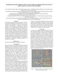
2. DEVELOPMENT OF THERMAL
MODELS OF EDLC
3D geometrical model of EDLC capacitor with
minimal complexity is shown on fig.5. It is representing
the scroll coil of mentioned sandwich structure (fig.1)
with diameter of 28 mm and height of 125 mm.
Compressed foils on top and bottm side are made from
extruded aluminum and have prepared area for electrical
contacts connection. The core of EDLC is separated from
aluminum chat through electrolyte layer.
Fig.5. Minimal complexity model of 1xEDLC
Each subdomain of EDLC has physical thermal
coefficients defined using material libraries from
COMSOL heat-transfer module [3]. Coefficient of core’s
thermal conductivity creates tensor of 2 grade in which
part of axial and radial thermal conductivity are being

included. For the higher accuracy of results from thermal
simulations we decided to develop also other models
whose geometrical properties will be in the closer
proximity to real physical sample. Next figure is showing
1xEDLC improved complexity model.
Fig.6. Improved complexity model of 1xEDLC
3. RESULTS AND COMPARISSONS OF
SIMULATION AND MEASUREMENT
EXPERIMENTS
Surroundings of EDLC model is air with temperature
of Tamb = 27,3 °C. Heat power in the core EDLC was set
to Ploss = 0,56 W. Next figure is showing result from
simulation experiment of simple complexity model for
steady state operation.
Fig.7. Interpretation of temperature distribution in whole
volume of EDLC - simple complexity model,
Ploss = 0,56 W, T amb = 27,3 °C
These results have been compared to experimental
measurement of physical sample. The parameters of
experimental measurement where the same as during
simulation experiment so Iload = 30 A, DCREDLC = 0,63
mΩ, Ploss = 0,56 W, Tamb = 27,3 °C. Charging process of
capacitor lasts 51 sec. with applied voltage of 2,5 V,
discharge process starts after 0,5 sec. and lasts 51 sec.
with applied voltage of 0 V. Next figure is showing result
from thermal measurement of physical sample.
Fig.8. Result from experimental measurement of EDLC,
Ploss = 0,56 W, T amb = 27,3 °C
Relative error between simulation and measurement for
subdomains - core of EDLC and case of EDLC, were
computed based on next equation:
T
rel_
err
∇T
T
= =
T
amb
core_
meas
T
−T
amb
core_
sim
=
31,
8−31,
987
= −0,
68%
27,
3
Table 1. Relative errors between simulation (simple model)
and measurement for subdomain CORE and CASE of EDLC
IRMS [A] Ploss [W] Trel_error
CORE 30A 0,561 -0,68 %
CASE 30A 0,561 -5,32 %
CORE 50A 1,33 -0,34 %
CASE 50A 1,33 -9,5 %
As was previously mentioned, facing requirements on
higher accuracy of simulation model, we decided to
develop improved complexity model. This model has
against simple complexity model two added subdomains:
aluminum coat, and air between aluminum coat and
minimal complexity model (fig.6.). The problems which
became into account after adding this subdomains was
increased number of total elements of computation mesh
(from 10 4 to 10 5 ). This fact has reflected into longer
computation time. Therefore the optimization of mesh
size manually have been done to improve computational
time whereby, better accuracy of model had to be
maintained.
Comparisons of results from simulation of minimal
complexity and improved complexity model are shown
on fig.8. The figure represents dependency of temperature
distribution in the core of ELDC in x-cut direction in the
middle of EDLC height. From fig.9. it can be seen that
due to improvement of 1xEDLC model the temperature

difference between core, and between can of EDLC is
much higher. This is caused due to air layer, which is
located between aluminum coat and minimal complexity
model (see fig.6.). From this simulation experiment it is
clear to say that aluminum coat (width = 0,5mm) and air
gap (width = 0,5mm) are causing that temperature inside
of EDLC is higher compared to minimal complexity
model by 3,74 ºC at Ploss = 1,62 W.
Next we have compared simulation results of
improved complexity model at conditions which were
similar to the conditions for simple complexity model.
One important change came into account, DCR - series
resistivity of EDLC of physical sample was changed due
to several non-specified reasons. We would like to note,
that reference measuring points have been changed
against first experiments (fig.10). The results from this
comparisons are listed in table 2.
Fig.10. Reference measuring points for verifications of
improved complexity model
Table 2. Relative errors between simulation (improved model)
and measurement for reference measuring points of EDLC
Face:
Fig.9. Plot of temperature of minimal and improved complexity model. Radial direction x- line for height (z) =0,04 m
Temperature
of Simulated
model [Ts]
Temperature of
Measured cell
[Tm]
Difference
(Ts-Tm)
Relative error
(Ts-Tm)/Ta
1_L_B 32,99 31,00 1,99 0,08
1_R_B 33,05 31,00 2,05 0,08
1_L_F 33,04 31,50 1,54 0,06
1_R_F 33,04 31,30 1,74 0,07
1_up 33,15 31,70 1,45 0,06
1_down 32,92 32,70 0,22 0,01
4. IMPACT OF COMPUTATION NET
DENSITY ON ACCURACY OF RESULTS
Previous experiments has confirmed that
improvements of simulation model of EDLC has led to
higher accuracy/lower relative error when compared to
measurements of physical sample. On the other hand
optimization of computational mesh was necessary due to
requirements on duration of simulation time. Therefore
we have also analyzed the accuracy of thermal field
computation in dependency on density of computation
net. For determination of relative error next equation have
been used:
(15)
T(x,extra fine) - temperature calculated in EDLC at
highest density of computation net
T(x,mesh size) - temperatture calculated in EDLC at
given density of computation net
In the COMSOL environment pre-defined mesh sizes
menu offers you selection of pre-defined mesh sizes that
automatically determine the parameters in the custom
mesh size menu.
Fig.11. Temperature in cross section area of EDLC in
dependeny on density of computation net

Pre - defined mesh size can generate from extremely fine
to extremenly coarse (extra fine, finer, fine, normal,
coarse, coarser, extra coarse). Fig.11 is showing line plot
of temperature in cross section area of EDLC (x-cut,
through diameter of EDLC). Figure represents
temperature in dependency on density of computation
net. Fig.12 is showing line plot of waveform of relative
error of temperature which was computed based on
equation (15).
Fig.12. Relative error of temperature in cross section area of
EDLC in dependeny on density of computation net
From this figure it can be seen that highest relative error
occurs at utilization of extremely coarse density and
minimal relative error occurs at extra fine density. This
results was expected and confirms our expectations. It
could be said that utilization of extra fine density of
computation net will bring best results. That is true but on
the other hand machine time for computation of solutions
also has to be taken into consideration.
Table 2. Machine time for computation of simulation results for
thermal distribution of EDLC (improved model)
Mesh size
Number of
elements
Machine time of
simulation [s]
EXTREMELY FINE 378 302 1 703, 280
EXTRA FINE 123 289 271,205
FINER 58 023 69,453
FINE 29 814 27,656
NORMAL 19 491 14,100
COARSE 6 421 3,437
COARSER 3 452 1,578
EXTRA COARSE
EXTREMELY
COARSE
1 765 Unsuccessfull
computation
620 0,437
Therefore we have analyzed also machine time
calculation in dependency on density of computation net.
Table 3 is showing mentioned results. It can be seen that
targeting relative error around 0,05% it is sufficient to
utilize finer or fine mesh size. In comparisons with
extremely fine settings the error is higher by around
0,04% but computation time is lowered by 98%. This is
very important result almost for applications and/or
research where high number of simulation experiments
have to be made in less time but have to have high
accuracy level.
5. CONCLUSION
This paper describes methodology of design of
thermal model of supercapacitor which is electrolytic
dual layer type. After developement of mathematical
model we have design thermal model in COMSOL 3.5a
environment. Next we have performed simulation
experiments which were compared to exact
measurements of physical sample. Targeting higher
accuracy of thermal model for future purposes we have
designed second model with improved complexity. In this
way we were able to aim higher accuracy when compared
to experimental measurements, but on the other hand
complexity of model became critical in the meanings of
density of computation net. Therefore we have analyzed
relationship between relative error, density of
computation net and computational time. From results it
is clear that for requested accuracy the fine settings of net
density is very sufficient. Almost this setting secures very
good accordance to experimental measurements with low
value of relative error. In next steps we are going to
develop thermal models with higher number of EDLC
cells. For these purposes the analysis of net density is
very necessary.
Acknowledgements
The authors wish to thank to projects from national
grant agency APVV nr. APVV-0535-07 nr. VMSP-P-
0085-09 and nr. LPP-0366-09
6. REFERENCES
[1] Sam G. Parler, Jr., Laird L. Macomber: Predicting
Operating Temperature and Expected
Lifetime of Aluminum-Electrolytic Bus
Capacitors with Thermal Modeling, Powersystems
World, November 1999
[2] Hargaš, L., Hrianka, M., Lakatoš, J., Koniar, D.:
Heat fields modelling and verification of
electronic parts of mechatronics systems,
Metalurgija (Metalurgy), Vol. 49 (2/2010), ISSN
1334-2576
[3] COMSOL: Multiphysics user guide