

Finite element calculations for the helium atom∗ 1 Introduction
Finite element calculations for the helium atom∗ 1 Introduction
Finite element calculations for the helium atom∗ 1 Introduction

You also want an ePaper? Increase the reach of your titles
YUMPU automatically turns print PDFs into web optimized ePapers that Google loves.
all states. The grid points are:<br />
1s1s 1 S : 0.0, 0.05, 0.1, 0.15, 0.2, 0.3, 0.4, 0.5, 0.6, 0.7, 0.8, 1.0, 1.2, 1.6,<br />
2.0, 2.6, 3.2, 4.2, 6.0, 9.0, 15.0;<br />
− 1.0, −0.6, −0.2, 0.2, 0.6, 1.0;<br />
1s2s 1 S : 0.0, 0.1, 0.2, 0.3, 0.4, 0.5, 0.6, 0.7, 0.8, 1.0, 1.2, 1.4, 1.6, 1.8, 2.0,<br />
2.2, 2.4, 2.6, 3.0, 3.4, 3.8, 4.2, 4.8, 5.6, 8.0, 11.5, 15.0, 20.0;<br />
− 1.0, −0.5, 0.5, 1.0;<br />
1s2s 3 S : 0.0, 0.05, 0.1, 0.2, 0.3, 0.4, 0.5, 0.6, 0.7, 0.8, 0.9, 1.0, 1.2, 1.4, 1.6,<br />
1.8, 2.0, 2.2, 2.4, 2.6, 2.8, 3.0, 3.2, 3.4, 3.6, 4.0, 4.5, 5.5, 7.0, 10.0, 13.0,<br />
16.0, 20.0, 25.0;<br />
− 1.0, 0.0, 1.0;<br />
1s2p 3 P : 0.0, 0.2, 0.4, 0.6, 0.8, 1.0, 1.2, 1.4, 1.6, 1.8, 2.2, 2.6, 3.0, 3.6, 5.0, 7.0,<br />
10.0, 15.0, 20.0, 25.0;<br />
− 1.0, 0.0, 1.0;<br />
1s3d 3 D : 0.0, 0.2, 0.4, 0.6, 1.0, 1.6, 2.2, 3.0, 4.0, 6.0, 9.0, 13.0, 18.0, 24.0, 30.0;<br />
− 1.0, 0.0, 1.0;<br />
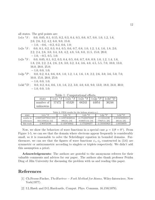
Table 1: Computational ef<strong>for</strong>ts.<br />
state 1s1s 1 S 1s2s 1 S 1s2s 3 S 1s2p 3 P 1s3d 3 D<br />
number of 57472 65320 68243 44954 36246<br />
unknowns<br />
Table 2: FEM results <strong>for</strong> <strong>the</strong> <strong>helium</strong> atom(a.u.).<br />
state 1s1s 1 S 1s2s 1 S 1s2s 3 S 1s2p 3 P 1s3d 3 D<br />
results in -2.90372437703411959 -2.1459740460544 -2.1752293782367 -2.133164190 -2.055636309453<br />
references 83111594(4) [12] 188(21) [10] 913037(13) [10] 77927(1) [35] 261(4) [35]<br />
this work -2.903724106 -2.1459740042 -2.1752293277 -2.1331633824 -2.05558078<br />
Now, we show <strong>the</strong> behaviors of wave functions in a special case µ = 1(θ = 0 ◦ ). From<br />
Figure 1-5, we can see that <strong>the</strong> domain where electrons appear frequently is considerably<br />
small, so it is reasonable to solve <strong>the</strong> Schrödinger equation in bounded domains. Fur<strong>the</strong>rmore,<br />
we can see that <strong>the</strong> figures of wave functions ψs, ψp constructed in (3.6) are<br />
symmetric or antisymmetric according to singlets or triplets respectively. We didn’t add<br />
this assumption a priori.<br />
Acknowledgements: The authors are grateful to <strong>the</strong> anonymous referees <strong>for</strong> <strong>the</strong>ir<br />
valuable comments and advices <strong>for</strong> our paper. The authors also thank professor Peizhu<br />
Ding of Jilin University <strong>for</strong> discussing <strong>the</strong> problem with us and reading this paper.<br />
References<br />
[1] Ch.Froese-Fischer, T heHartree − F ock Method <strong>for</strong>Atoms, Wiley-Intersciece, New<br />
York(1977).<br />
[2] I.L.Hawk and D.L.Hardcastle, Comput. Phys. Commun. 16,159(1979).<br />
12