Finite element calculations for the helium atom∗ 1 Introduction

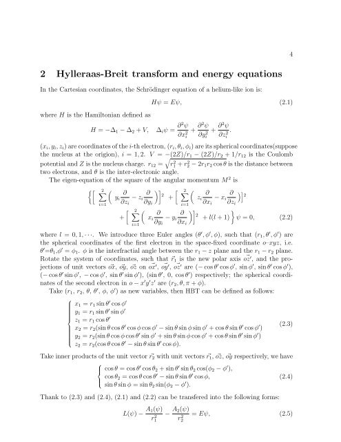
2 Hylleraas-Breit transform and energy equations
In the Cartesian coordinates, the Schrödinger equation of a helium-like ion is:
where H is the Hamiltonian defined as
H = −∆1 − ∆2 + V, ∆iψ = ∂2 ψ
∂x 2 i
Hψ = Eψ, (2.1)
+ ∂2 ψ
∂y 2 i
+ ∂2ψ ∂z2 .
i
(xi, yi, zi) are coordinates of the i-th electron, (ri, θi, φi) are its spherical coordinates(suppose
the nucleus at the origion), i = 1, 2. V = −(2Z)/r1 − (2Z)/r2 + 1/r12 �
is the Coulomb
potential and Z is the nucleus charge. r12 = r2 1 + r2 2 − 2r1r2 cos θ is the distance between
two electrons, and θ is the inter-electronic angle.
The eigen-equation of the square of the angular momentum M 2 is
��
�2
�
i=1
yi
�� �
∂ ∂
�2
�
2 ∂ ∂ ��
2
− zi + zi − xi
∂zi ∂yi
i=1 ∂xi ∂zi
�
�2
�
�� �
∂ ∂ 2
+ xi − yi + l(l + 1) ψ = 0, (2.2)
∂yi ∂xi
i=1
where l = 0, 1, · · ·. We introduce three Euler angles (θ ′ , φ ′ , φ), such that (r1, θ ′ , φ ′ ) are
the spherical coordinates of the first electron in the space-fixed coordinate o–xyz, i.e.
θ ′ =θ1,φ ′ = φ1. φ is the interfractial angle between the r1 − z plane and the r1 − r2 plane.
Rotate the system of coordinates, such that �r1 is the new polar axis oz � ′ , and the projections
of unit vectors �ox, �oy, �oz on ox � ′ , oy � ′ , oz � ′ are (− cos θ ′ cos φ ′ , sin φ ′ , sin θ ′ cos φ ′ ),
(− cos θ ′ sin φ ′ , − cos φ ′ , sin θ ′ sin φ ′ ), (sin θ ′ , 0, cos θ ′ ) respectively; the spherical coordinates
of the second electron in o − x ′ y ′ z ′ are (r2, θ, π + φ).
Take (r1, r2, θ, θ ′ , φ, φ ′ ) as new variables, then HBT can be defined as follows:
⎧
x1 = r1 sin θ
⎪⎨
⎪⎩
′ cos φ ′
y1 = r1 sin θ ′ sin φ ′
z1 = r1 cos θ ′
x2 = r2(sin θ cos θ ′ cos φ cos φ ′ − sin θ sin φ sin φ ′ + cos θ sin θ ′ cos φ ′ )
y2 = r2(sin θ cos φ cos θ ′ sin φ ′ + sin θ sin φ cos φ ′ + cos θ sin θ ′ sin φ ′ )
z2 = r2(cos θ cos θ ′ − sin θ sin θ ′ (2.3)
cos φ).
Take inner products of the unit vector �r2 with unit vectors �r1, �oz, �oy respectively, we have
⎧
⎪⎨
⎪⎩
cos θ = cos θ ′ cos θ2 + sin θ ′ sin θ2 cos(φ2 − φ ′ ),
cos θ2 = cos θ cos θ ′ − sin θ sin θ ′ cos φ,
sin θ sin φ = sin θ2 sin(φ2 − φ ′ ).
Thank to (2.3) and (2.4), (2.1) and (2.2) can be transfered into the following forms:
L(ψ) − A1(ψ)
r 2 1
− A2(ψ)
r 2 2
4
(2.4)
= Eψ, (2.5)