Finite Element Method 2D heat conduction 1
Finite Element Method 2D heat conduction 1
Finite Element Method 2D heat conduction 1

Create successful ePaper yourself
Turn your PDF publications into a flip-book with our unique Google optimized e-Paper software.
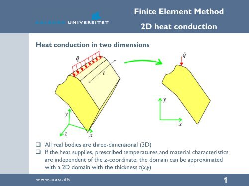
Heat <strong>conduction</strong> in two dimensions<br />
<strong>Finite</strong> <strong>Element</strong> <strong>Method</strong><br />
<strong>2D</strong> <strong>heat</strong> <strong>conduction</strong><br />
� All real bodies are three-dimensional (3D)<br />
� If the <strong>heat</strong> supplies, prescribed temperatures and material characteristics<br />
are independent of the z-coordinate, the domain can be approximated<br />
with a <strong>2D</strong> domain with the thickness t(x,y)<br />
1
<strong>Finite</strong> <strong>Element</strong> <strong>Method</strong><br />
<strong>2D</strong> <strong>heat</strong> <strong>conduction</strong><br />
Discretization into two-dimensional finite elements<br />
� The body is discretized with a number of finite elements<br />
� They can be triangular or quadrilateral<br />
� Straight or curved element sides<br />
2
Today’s elements<br />
� Melosh element<br />
� Four nodes<br />
� Only right angles<br />
� Must be aligned with the<br />
coordinate axes<br />
� Constant strain triangle (CST)<br />
� Three nodes<br />
� Arbitrary angles<br />
� Arbitrary orientation<br />
� Isoparametric four-node<br />
element<br />
� Four nodes<br />
� Arbitrary angles<br />
� Arbitrary orientation<br />
<strong>Finite</strong> <strong>Element</strong> <strong>Method</strong><br />
<strong>2D</strong> <strong>heat</strong> <strong>conduction</strong><br />
<strong>Element</strong> node at the corner<br />
(vertex)<br />
<strong>Element</strong> side (edge)<br />
<strong>Element</strong> interior<br />
3
Other useful elements<br />
<strong>Finite</strong> <strong>Element</strong> <strong>Method</strong><br />
<strong>2D</strong> <strong>heat</strong> <strong>conduction</strong><br />
� Triangular six-node element with straight edges and<br />
midside nodes (Lecture 8 + 9)<br />
� Triangular isoparametric six-node element with curved<br />
edges and off-midside nodes<br />
� Isoparametric eight-noded elements with straight edges<br />
and midside nodes<br />
� Isoparametric eight-noded elements with curved edges<br />
and off-midside nodes (Lecture 8 + 9)<br />
4
The patch test<br />
<strong>Finite</strong> <strong>Element</strong> <strong>Method</strong><br />
<strong>2D</strong> <strong>heat</strong> <strong>conduction</strong><br />
� The main exercise of today is the patch test. You will program its<br />
main parts and use it to verify that the elements work properly.<br />
� A patch test should include at least one<br />
internal node<br />
� The patch test should be as<br />
unconstrained as possible, i.e. the<br />
temperature should be specified<br />
at only one node.<br />
� Before we go into the equations of <strong>2D</strong><br />
<strong>heat</strong> <strong>conduction</strong>, you must now start<br />
MatLab and do a small exercise.<br />
5
<strong>Finite</strong> <strong>Element</strong> <strong>Method</strong><br />
<strong>2D</strong> <strong>heat</strong> <strong>conduction</strong><br />
Exercise: Program and plot the geometry and topology of a<br />
<strong>2D</strong> patch test for the Melosh, CST and ISO4 elements<br />
Melosh etype = 1 CST etype = 3 Iso4 etype = 7<br />
Coord = [ x1 y1 z1 ; x2 y2 y3 ; …. ] % Nodal coordinates in file “Coordinates.m”<br />
Top = [ etype section etc ] % for each element in the file “Topology.m”<br />
Plot by executing the line “visualize<strong>2D</strong>”<br />
6
Basic steps of the finite-element method (FEM)<br />
1. Establish strong formulation<br />
� Partial differential equation<br />
2. Establish weak formulation<br />
<strong>Finite</strong> <strong>Element</strong> <strong>Method</strong><br />
<strong>2D</strong> <strong>heat</strong> <strong>conduction</strong><br />
� Multiply with arbitrary field and integrate over element<br />
3. Discretize over space<br />
� Mesh generation<br />
4. Select shape and weight functions<br />
� Galerkin method<br />
5. Compute element stiffness matrix<br />
� Local and global system<br />
6. Assemble global system stiffness matrix<br />
7. Apply nodal boundary conditions<br />
� temperature/flux/forces/forced displacements<br />
8. Solve global system of equations<br />
� Solve for nodal values of the primary variables (displacements/temperature)<br />
9. Compute temperature/stresses/strains etc. within the element<br />
� Using nodal values and shape functions<br />
7
<strong>Finite</strong> <strong>Element</strong> <strong>Method</strong><br />
<strong>2D</strong> <strong>heat</strong> <strong>conduction</strong><br />
Step 1: Establish strong formulation for <strong>2D</strong> <strong>heat</strong> <strong>conduction</strong><br />
(OP pp. 76-84)<br />
½ ¾ ·<br />
qx J<br />
Heat flow (flux) vector q =<br />
qy m<br />
Boundary normal<br />
2 ¸<br />
½ ¾<br />
s<br />
nx<br />
n = jnj = 1<br />
Heat flow out of the boundary (the flux)<br />
qn = q ¢ n = q T n<br />
1D:<br />
<strong>2D</strong>:<br />
ny<br />
8
The constitutive relation in matrix notation:<br />
, material isotropy leads to<br />
<strong>Finite</strong> <strong>Element</strong> <strong>Method</strong><br />
<strong>2D</strong> <strong>heat</strong> <strong>conduction</strong><br />
9
Q is internal<br />
<strong>heat</strong> supply<br />
[J/m 3 s]<br />
Divergence:<br />
t is the<br />
thickness [m]<br />
<strong>Finite</strong> <strong>Element</strong> <strong>Method</strong><br />
<strong>2D</strong> <strong>heat</strong> <strong>conduction</strong><br />
Energy conservation and a time independent problem leads to: The amount of<br />
<strong>heat</strong> (energy) supplied to the body per unit of time must equal the amount of<br />
<strong>heat</strong> leaving the body per unit time:<br />
Rearranging leads to<br />
Gauss’ divergence theorem (OP p. 73)<br />
Prescribed<br />
quantities<br />
10
Insertion of the constitutive relation leads to the strong<br />
formulation:<br />
Boundary<br />
conditions<br />
Written out, the strong form for stationary <strong>2D</strong> <strong>heat</strong><br />
<strong>conduction</strong> is<br />
<strong>Finite</strong> <strong>Element</strong> <strong>Method</strong><br />
<strong>2D</strong> <strong>heat</strong> <strong>conduction</strong><br />
Prescribed<br />
quantities<br />
11
<strong>Finite</strong> <strong>Element</strong> <strong>Method</strong><br />
<strong>2D</strong> <strong>heat</strong> <strong>conduction</strong><br />
Step 2: Establish weak formulation for <strong>2D</strong> <strong>heat</strong> <strong>conduction</strong><br />
(Cook pp. 136-137, 151), (OP Chapter 5, pp. 84-86)<br />
Multiply the strong formulation with a weight<br />
function v(x,y) and integrate over the domain<br />
The Green-Gauss theorem (OP p. 74)<br />
Inserting into the first equation while replacing<br />
yields<br />
Prescribed<br />
quantities<br />
12
The boundary integral is split into two terms to reflect<br />
the two different types of boundary conditions<br />
Insertion into the top equation followed by<br />
rearranging leads to the weak form of <strong>2D</strong> <strong>heat</strong> flow<br />
<strong>Finite</strong> <strong>Element</strong> <strong>Method</strong><br />
<strong>2D</strong> <strong>heat</strong> <strong>conduction</strong><br />
Prescribed<br />
quantities<br />
Boundary conditions Internal <strong>heat</strong> supply (<strong>heat</strong> load)<br />
13
Basic steps of the finite-element method (FEM)<br />
1. Establish strong formulation<br />
� Partial differential equation<br />
2. Establish weak formulation<br />
<strong>Finite</strong> <strong>Element</strong> <strong>Method</strong><br />
<strong>2D</strong> <strong>heat</strong> <strong>conduction</strong><br />
� Multiply with arbitrary field and integrate over element<br />
3. Discretize over space<br />
� Mesh generation<br />
4. Select shape and weight functions<br />
� Galerkin method<br />
5. Compute element stiffness matrix<br />
� Local and global system<br />
6. Assemble global system stiffness matrix<br />
7. Apply nodal boundary conditions<br />
� temperature/flux/forces/forced displacements<br />
8. Solve global system of equations<br />
� Solve for nodal values of the primary variables (displacements/temperature)<br />
9. Compute temperature/stresses/strains etc. within the element<br />
� Using nodal values and shape functions<br />
14
Step 3: Discretize over space<br />
Now the domain is discretized into a number of finite<br />
elements. This determines the mesh coordinates and<br />
the element topology, i.e. the matrices coord and Top in<br />
our MatLab program.<br />
Here it is illustrated with a single Melosh element.<br />
<strong>Finite</strong> <strong>Element</strong> <strong>Method</strong><br />
<strong>2D</strong> <strong>heat</strong> <strong>conduction</strong><br />
15
Step 4: Weight and shape functions<br />
The Galerkin method is chosen. This means that the<br />
main variable (the temperature) and the weight function<br />
v(x,y) are interpolated using the same interpolation<br />
functions<br />
Known shape functions<br />
(depends only on x and y)<br />
Examples:<br />
<strong>Finite</strong> <strong>Element</strong> <strong>Method</strong><br />
<strong>2D</strong> <strong>heat</strong> <strong>conduction</strong><br />
Unknown nodal values<br />
16
The weak form can now be written as<br />
Noticing that v and a are constants, rearranging yields<br />
<strong>Finite</strong> <strong>Element</strong> <strong>Method</strong><br />
<strong>2D</strong> <strong>heat</strong> <strong>conduction</strong><br />
Because v is arbitrary the parenthesis term must vanish (equal zero)<br />
where<br />
17
Degrees of<br />
freedom, dof<br />
<strong>Finite</strong> <strong>Element</strong> <strong>Method</strong><br />
<strong>2D</strong> <strong>heat</strong> <strong>conduction</strong><br />
In order to be able to write the equations in a compact form the following<br />
terms are introduced<br />
The equations can now be written as<br />
Example: The Melosh <strong>heat</strong> <strong>conduction</strong> element:<br />
The stiffness matrix<br />
Boundary terms (boundary load vector)<br />
Internal load vector<br />
18
The definition of the <strong>heat</strong> flux was<br />
With the finite element formulation we have<br />
This gives us the flux within the element as<br />
<strong>Finite</strong> <strong>Element</strong> <strong>Method</strong><br />
<strong>2D</strong> <strong>heat</strong> <strong>conduction</strong><br />
19
Shape and weight functions<br />
Example: The melosh element<br />
Notice that N i vary linearly along element edges.<br />
Example:<br />
This ensures inter-element combatibility, i.e. no gaps<br />
and no overlapping:<br />
<strong>Finite</strong> <strong>Element</strong> <strong>Method</strong><br />
<strong>2D</strong> <strong>heat</strong> <strong>conduction</strong><br />
20
<strong>Finite</strong> <strong>Element</strong> <strong>Method</strong><br />
<strong>2D</strong> <strong>heat</strong> <strong>conduction</strong><br />
Exercise: compute and program the Melosh stiffness matrix<br />
Assumptions: D and t are constant.<br />
<strong>Element</strong> width: 2a, height 2b<br />
Steps:<br />
1. Compute B-matrix<br />
2. Carry out matrix multiplication<br />
3. Integrate each element of the matrix product to<br />
obtain K<br />
4. Program K into the file KmeloshHeat.m<br />
5. A test value with the parameters, 2a = 2, 2b = 1,<br />
t = 1.3, k xx = 4.56, k yy = 3.8 is :<br />
21
Can only contain<br />
nodal values<br />
Unit: J/s<br />
Boundary load vector<br />
Can only contain values at nodes. So uniform <strong>heat</strong> supplies<br />
must be converted into nodal loads<br />
Prescribed term<br />
Reactions<br />
Example: constant <strong>heat</strong> supply between nodes 1 and 2<br />
<strong>Finite</strong> <strong>Element</strong> <strong>Method</strong><br />
<strong>2D</strong> <strong>heat</strong> <strong>conduction</strong><br />
Remember: If <strong>heat</strong> is transferred into the domain, q is negative<br />
22
<strong>Finite</strong> <strong>Element</strong> <strong>Method</strong><br />
<strong>2D</strong> <strong>heat</strong> <strong>conduction</strong><br />
Exercise: Calculate f b with triangular <strong>heat</strong> load<br />
The <strong>heat</strong> load varies linearly from zero at node 2 to the<br />
value q 3 at node 3<br />
Can only contain<br />
nodal values<br />
Prescribed term<br />
Steps:<br />
1. Find the expression for the <strong>heat</strong> load as a<br />
function of the coordinates q(x,y)<br />
2. Carry out the integration as shown on the<br />
previous slide.<br />
Remember: If <strong>heat</strong> is transferred into the domain, q is negative<br />
23
Q is internal<br />
<strong>heat</strong> supply<br />
[J/m 3 s]<br />
Internal load vector<br />
Can only contain values at nodes. So internal <strong>heat</strong> supplies<br />
must be converted into nodal loads<br />
Example: constant internal <strong>heat</strong> supply in a Melosh element<br />
<strong>Finite</strong> <strong>Element</strong> <strong>Method</strong><br />
<strong>2D</strong> <strong>heat</strong> <strong>conduction</strong><br />
<strong>Element</strong> area A = 4 ab<br />
24
Step 6: Assembling<br />
<strong>Finite</strong> <strong>Element</strong> <strong>Method</strong><br />
<strong>2D</strong> <strong>heat</strong> <strong>conduction</strong><br />
� The assembling procedure is exactly the same as in the last lecture:<br />
1. Determine the local stiffness matrix<br />
2. determine the global number of dof corresponding to the local dof for the element<br />
3. add the components of the local stiffness matrix to the rows and columns of the<br />
global stiffness matrix corresponding to the global dof numbers<br />
4. repeat 1-3 until all contributions from all elements have been added.<br />
� In MatLab this is done in assemblering.m<br />
K(gDof,gDof) = K(gDof,gDof) + Ke;<br />
25
<strong>Finite</strong> <strong>Element</strong> <strong>Method</strong><br />
<strong>2D</strong> <strong>heat</strong> <strong>conduction</strong><br />
� In order to be able to create a global system matrix we need to give<br />
information about<br />
� Material for each element<br />
� Section dimensions for each element<br />
� Coordinates for each node (and a numbering)<br />
� Topology for each element (which nodes are in the element)<br />
� dof numbering is given from the node numbering and number of dofs per node (one<br />
in this case)<br />
� See calc_globdof.m for numbering of global dof<br />
� ElemDof = [neDof1 GDof1 GDof2 ...]<br />
� dof numbering of each element<br />
� GlobDof = [Gnode1 GDof1 GDof2 ...]<br />
� dof numbering of each node (used for plotting)<br />
� nDof = total number of Dof<br />
26
Remember: If <strong>heat</strong> is<br />
transferred into the<br />
domain, q is negative<br />
Example of assembling the load vector<br />
Total <strong>heat</strong> load vector<br />
<strong>Finite</strong> <strong>Element</strong> <strong>Method</strong><br />
<strong>2D</strong> <strong>heat</strong> <strong>conduction</strong><br />
The global matrices are assembled in exactly the same way as with the bar elements of the previous<br />
lecture. Here an example of the assembly of the load vector of a two element system is shown<br />
The thicknesses of the two<br />
elements are identical<br />
27
<strong>Finite</strong> <strong>Element</strong> <strong>Method</strong><br />
<strong>2D</strong> <strong>heat</strong> <strong>conduction</strong><br />
Exercise: Program and plot the results of a <strong>2D</strong> patch test for<br />
the Melosh element<br />
Compare with the analytical solution:<br />
Hint: on the colorplot the temperatures can be found by<br />
activating the figure and typing “colorbar” at the command line<br />
t = 1.2 m, k xx = k yy = 3 J/Cms<br />
Steps<br />
1. Program the geometry (done earlier today)<br />
2. Determine nodal <strong>heat</strong> supplies q 3, q 6, and q 9<br />
3. Determine nodal <strong>heat</strong> supply q 4 and q 7 (We<br />
want T = 0 on the left boundary, x = 0)<br />
4. Make the appropriate programming in<br />
Topology.m and BoundaryConditions.m<br />
5. Plot by executing the line “visualizeD2<br />
28
<strong>Finite</strong> <strong>Element</strong> <strong>Method</strong><br />
<strong>2D</strong> <strong>heat</strong> <strong>conduction</strong><br />
Why use other elements than the Melosh element?<br />
• The Melosh element must be rectangular and<br />
positioned along the coordinate axes<br />
• It is therefore not very good at approximating<br />
boundaries not aligned with the coordinate axes<br />
• Conclusion: The Melosh element is not very flexible<br />
Why use triangular elements?<br />
• Triangular elements can be rotated arbitrarily<br />
• They can therefore approximate boundaries not aligned<br />
with coordinate axes well.<br />
• It is relatively simple to make a computer code that<br />
meshes an arbitrary area with triangles.<br />
Next: The constant strain triangle (CST)<br />
• The name stems from its original development within structural mechanics<br />
• In <strong>heat</strong> <strong>conduction</strong> analysis the name “constrant flux triangle” would be<br />
appropriate<br />
29
<strong>Finite</strong> <strong>Element</strong> <strong>Method</strong><br />
<strong>2D</strong> <strong>heat</strong> <strong>conduction</strong><br />
Preliminary: Natural coordinates (Area coordinates)<br />
• For general triangular elements it has proven useful<br />
to derive the stiffness matrix using the so-called<br />
“natural coordinates” also referred to as “area<br />
coordinates<br />
Point P defines three areas. These define the<br />
natural coordinate of the point<br />
The following constraint applies<br />
Examples:<br />
<strong>Element</strong> centroid:<br />
Node 1<br />
Node 3<br />
30
The relation between natural and cartesian<br />
coordinates is<br />
In matrix notation<br />
With the coordinate transformation matrix A<br />
here<br />
The element area can be found by<br />
<strong>Finite</strong> <strong>Element</strong> <strong>Method</strong><br />
<strong>2D</strong> <strong>heat</strong> <strong>conduction</strong><br />
31
Differentiation in natural coordinates<br />
A function N (e.g. a shape function) is expressed in<br />
natural coordinates, N(� 1, � 2, � 3). The chain rule<br />
then gives us<br />
With the coordinate transformation<br />
we get<br />
<strong>Finite</strong> <strong>Element</strong> <strong>Method</strong><br />
<strong>2D</strong> <strong>heat</strong> <strong>conduction</strong><br />
32
Integration in natural coordinates<br />
A polynomial function expressed in natural<br />
coordinates, f(� 1, � 2, � 3) can easily be integrated over<br />
the element area using the formula<br />
Example:<br />
<strong>Finite</strong> <strong>Element</strong> <strong>Method</strong><br />
<strong>2D</strong> <strong>heat</strong> <strong>conduction</strong><br />
33
Shape functions for the CST-element<br />
The shape functions for the CST-element in natural coordinates<br />
are very simple:<br />
The temperature in the element interior is then given by<br />
The stiffness matrix is again given by<br />
with<br />
<strong>Finite</strong> <strong>Element</strong> <strong>Method</strong><br />
<strong>2D</strong> <strong>heat</strong> <strong>conduction</strong><br />
34
<strong>Finite</strong> <strong>Element</strong> <strong>Method</strong><br />
<strong>2D</strong> <strong>heat</strong> <strong>conduction</strong><br />
Exercise: Calculate and program the stiffness matrix<br />
of the <strong>heat</strong> <strong>conduction</strong> CST-element<br />
Steps<br />
1. Determine the derivatives in the B-matrix<br />
2. Setup the B-matrix. Think about and explain why the element<br />
name “constant flux element” is appropriate (hint on slide 18)<br />
3. Carry out the matrix multiplication indicated on the previous<br />
slide.<br />
4. Integrate over the element area to obtain the stiffness matrix<br />
K<br />
5. Program the stiffness matrix into the file K_CST_Heat.m<br />
6. A test value with the parameters (x 1, x 2, x 3) = (1, 3, -1), (y 1,<br />
y 2, y 3) = (0, 2, 1), t = 1.3, k xx = 4.7 and k yy = 5.1 is<br />
35
<strong>Finite</strong> <strong>Element</strong> <strong>Method</strong><br />
<strong>2D</strong> <strong>heat</strong> <strong>conduction</strong><br />
Exercise: Program and plot the results of a <strong>2D</strong> patch test for<br />
the CST element<br />
Compare with the analytical solution:<br />
Hint: on the colorplot the temperatures can be found by<br />
activating the figure and typing “colorbar” at the command line<br />
t = 1.2 m, k xx = k yy = 3 W/ Cm<br />
Steps<br />
1. Program the geometry (done earlier today)<br />
2. Determine nodal <strong>heat</strong> supplies q 3, q 6, and q 9<br />
3. Determine nodal <strong>heat</strong> supply q 4 and q 7 (We<br />
want T = 0 on the left boundary, x = 0)<br />
4. Make the appropriate programming in<br />
Topology.m and BoundaryConditions.m<br />
5. Plot by executing the line “visualizeD2<br />
36
The isoparametric four node element (Iso4)<br />
• A quadrilateral element which can be distorted from<br />
the rectangular shape and rotated arbitrarily in the<br />
plane<br />
• Introduces several important concepts in finite element<br />
theory, such as<br />
• Isoparametric coordinates<br />
• Parent and global domain<br />
• The Jacobian matrix and the Jacobian<br />
• Numerical integration by Gauss quadrature<br />
• The isoparametric formulation forms the basis for<br />
nearly all the elements in practical use<br />
<strong>Finite</strong> <strong>Element</strong> <strong>Method</strong><br />
<strong>2D</strong> <strong>heat</strong> <strong>conduction</strong><br />
37
Parent and global domain<br />
• For general quadrilateral elements is has proven<br />
useful to formulate the stiffness matrix using the<br />
isoparametric formulation.<br />
• In the parent domain the element is always a<br />
square element with the side length 2.<br />
• The isoparametric coordinates � and � have their<br />
origin at the element centroid. This means that the<br />
vertex (corner) nodes have the coordinates (�,�):<br />
1: (-1,-1), 2: (1,-1), 3: (1,1) and 4: (-1,1)<br />
• In the global domain the nodes of the four node<br />
element have the coordinates: (x,y): 1: (x 1,y 1), 2:<br />
(x 2,y 2), 3: (x 3,y 3), and 4: (x 4,y 4).<br />
• The question is “how do we connect these two<br />
sets of coordinates?” (much in a similar way as we<br />
did with the triangle.)<br />
Note: with the natural coordinates of the triangle the coordinate<br />
limits were 0 � � 1, � 2, � 3 � 1. For the isoparametric coordinates<br />
they are -1 � �, � � 1<br />
<strong>Finite</strong> <strong>Element</strong> <strong>Method</strong><br />
<strong>2D</strong> <strong>heat</strong> <strong>conduction</strong><br />
Parent<br />
domain<br />
Global<br />
domain<br />
38
The isoparametric coordinate transformation<br />
• The idea is that we use the shape functions to<br />
interpolate the coordinates between the nodes Parent<br />
domain<br />
e.g.<br />
With the shape functions:<br />
Notice that these are the shape functions of the<br />
Melosh element with a = b = 1<br />
<strong>Finite</strong> <strong>Element</strong> <strong>Method</strong><br />
<strong>2D</strong> <strong>heat</strong> <strong>conduction</strong><br />
Global<br />
domain<br />
39
Temperature and flux interpolation<br />
As usual the temperature within the element is interpolated<br />
from the nodal values Parent<br />
domain<br />
The <strong>heat</strong> flux is also still given by<br />
with<br />
Problem: we have to find the derivatives of the<br />
shape functions with respect to the global (x,y)<br />
coordinates, but the shape functions are expressed<br />
in the isoparametric (�,�) coordinates. To overcome<br />
this problem we will define B as a product of two<br />
matrices:<br />
<strong>Finite</strong> <strong>Element</strong> <strong>Method</strong><br />
<strong>2D</strong> <strong>heat</strong> <strong>conduction</strong><br />
Global<br />
domain<br />
40
The matrix D N contains the derivatives of the shape<br />
functions with respect to the isoparametric coordinates<br />
With D N the temperature derivatives within the element can<br />
be found by<br />
If we wanted the temperature derivatives the (�,�)coordinates<br />
we were done now. But we need them in the<br />
(x,y) system in order to determine the <strong>heat</strong> flux. The<br />
transformation of derivatives from the (�,�) system into<br />
the (x,y) system is carried out by the inverse of the socalled<br />
“Jacobian matrix”, J -1<br />
<strong>Finite</strong> <strong>Element</strong> <strong>Method</strong><br />
<strong>2D</strong> <strong>heat</strong> <strong>conduction</strong><br />
Parent<br />
domain<br />
Global<br />
domain<br />
41
The Jacobian matrix<br />
The matrix J is called “the Jacobian matrix” and it relates<br />
the temperature derivatives in the two coordinate<br />
systems<br />
<strong>Finite</strong> <strong>Element</strong> <strong>Method</strong><br />
<strong>2D</strong> <strong>heat</strong> <strong>conduction</strong><br />
Parent<br />
domain<br />
The elements of J can be found by differentiating the temperature<br />
with respect to (�, �) by invoking the chain rule:<br />
Global<br />
domain<br />
This gives us the elements of J<br />
42
The Jacobian<br />
<strong>Finite</strong> <strong>Element</strong> <strong>Method</strong><br />
<strong>2D</strong> <strong>heat</strong> <strong>conduction</strong><br />
The inverse of J, which was needed in the expression for B,<br />
, can now be found by<br />
Parent<br />
domain<br />
where the determinant of J, which is often called “the<br />
Jacobian”, is given by<br />
The Jacobian can be regarded as a scale factor that relates<br />
infinitesimal areas in the parent domain and the global<br />
domain, see (Cook pp. 206 – 207), (OP pp. 376 – 380)<br />
Global<br />
domain<br />
43
Stiffness matrix for the Iso4 element<br />
The definition of the stiffness matrix was<br />
With the Jacobian matrix and its determinant we now have<br />
the tools to calculate the stiffness matrix of a<br />
isoparametric quadrilateral element.<br />
The integral is non-linear and can, in general, not be<br />
solved analytically. Therefore we must use numerical<br />
integration.<br />
As a remark it should be mentioned that the shape<br />
functions are still linear along the element sides. This<br />
means that boundary loads are distributed to the nodes<br />
in the same way as it was done with the Melosh element.<br />
<strong>Finite</strong> <strong>Element</strong> <strong>Method</strong><br />
<strong>2D</strong> <strong>heat</strong> <strong>conduction</strong><br />
Parent<br />
domain<br />
Global<br />
domain<br />
44
Numerical integration<br />
Our concern is to find the following integral numerically<br />
One way of doing this is to divide the domain in n equal<br />
intervals of equal width W, and sum up the contribution<br />
from n rectangular areas with the height given by the<br />
function value in the centre of the intervals<br />
A second method is analogous to the above but with<br />
varying interval widths W i<br />
Both methods will converge towards the exact integral<br />
when the number of intervals, n, increases.<br />
<strong>Finite</strong> <strong>Element</strong> <strong>Method</strong><br />
<strong>2D</strong> <strong>heat</strong> <strong>conduction</strong><br />
45
Gauss quadrature<br />
The position of the evaluation points x i and the size of the<br />
widths (also called weight factors) can be optimized with<br />
respect to the function that is integrated. For integrals of<br />
polynomials in the interval [-1 ; 1] this in known as the socalled<br />
Gauss quadrature. Notice that this is the interval we<br />
are interested in with isoparametric elements as the<br />
isoparametric coordinates -1 � �, � �1. With Gauss<br />
quadrature we can evaluate integrals as<br />
with the following positions and weights<br />
<strong>Finite</strong> <strong>Element</strong> <strong>Method</strong><br />
<strong>2D</strong> <strong>heat</strong> <strong>conduction</strong><br />
46
Gauss points and weights<br />
A polynomium of degree 2n – 1 is integrated exact with a<br />
Gauss quadrature of degree n.<br />
<strong>Finite</strong> <strong>Element</strong> <strong>Method</strong><br />
<strong>2D</strong> <strong>heat</strong> <strong>conduction</strong><br />
47
Gauss quadrature in two dimensions<br />
For the calculation of the stiffness matrix we need the<br />
Gauss quadrature in two dimensions. This is obtained as<br />
follows<br />
Example: Numerical integration of �(�,�) with Gauss<br />
order n = 2, which gives 2�2 = 4 points:<br />
<strong>Finite</strong> <strong>Element</strong> <strong>Method</strong><br />
<strong>2D</strong> <strong>heat</strong> <strong>conduction</strong><br />
48
<strong>Finite</strong> <strong>Element</strong> <strong>Method</strong><br />
<strong>2D</strong> <strong>heat</strong> <strong>conduction</strong><br />
Exercise: Numerical integration of two functions in <strong>2D</strong><br />
Steps<br />
1. Open NumIntExc_Lec34_student.m<br />
2. In the loop calculate the function value Φ at each Gauss point<br />
3. Sum the integral in the variable “numint”. Remember the weight functions (see the previous slide)<br />
4. Save the exact solution in the variable “int_exact”.<br />
5. Start with one Gausspoint, then two, and so on..<br />
6. Run the program by pressing F5.<br />
What is different about the two functions?<br />
� �1<br />
function 2: 1 �<br />
3<br />
�1 2<br />
2<br />
� 3 �<br />
function 1:<br />
exact solution<br />
�1<br />
�<br />
2��3 1 1<br />
��<br />
�1�1 � d�d�� 1<br />
2 2 ln5<br />
3<br />
exact solution<br />
� �� �<br />
� � � � �<br />
1 1<br />
��<br />
�1�1 � d�d��� 2<br />
49<br />
28<br />
3
<strong>Finite</strong> <strong>Element</strong> <strong>Method</strong><br />
<strong>2D</strong> <strong>heat</strong> <strong>conduction</strong><br />
Exercise: Calculate and program the stiffness matrix of the <strong>heat</strong><br />
<strong>conduction</strong> Iso4-element<br />
Steps<br />
1. Open the file K_QuadIso_Heat.m<br />
2. Setup a loop over the Gauss points<br />
3. Initiate the stiffness matrix as zeros<br />
4. Perform steps 5 to 9 inside a loop over the Gauss points<br />
5. Calculate the and setup the D N-matrix<br />
6. Calculate the Jacobian matrix<br />
7. Calculate the determinant of the Jacobian matrix<br />
8. Calculate the inverse Jacobian matrix<br />
9. Calculate the integral at the current Gauss point and add it to the current value of<br />
the stiffness matrix, Ke<br />
10. A test value with the parameters (x 1, x 2, x 3, x 4) = (1, 3, 3.5, -1), (y 1, y 2, y 3, y 4)<br />
= (0, -1, 1 1), t = 1.3, k xx = 4.7 and k yy = 5.1 n = 2 (Gauss order)<br />
50
<strong>Finite</strong> <strong>Element</strong> <strong>Method</strong><br />
<strong>2D</strong> <strong>heat</strong> <strong>conduction</strong><br />
Exercise: Program and plot the results of a <strong>2D</strong> patch test for<br />
the Iso4 element<br />
Compare with the analytical solution:<br />
Hint: on the colorplot the temperatures can be found by<br />
activating the figure and typing “colorbar” at the command line<br />
t = 1.2 m, k xx = k yy = 3 J/Cms<br />
Steps<br />
1. Program the geometry (done earlier today)<br />
2. Determine nodal <strong>heat</strong> supplies q 3, q 6, and q 9<br />
3. Determine nodal <strong>heat</strong> supply q 4 and q 7 (We<br />
want T = 0 on the left boundary, x = 0)<br />
4. Make the appropriate programming in<br />
Topology.m and BoundaryConditions.m<br />
5. Plot by executing the line “visualizeD2<br />
51
<strong>Finite</strong> <strong>Element</strong> <strong>Method</strong><br />
<strong>2D</strong> <strong>heat</strong> <strong>conduction</strong><br />
Exercise: Get familiar with the program and test the<br />
different elements<br />
We will now try to carry out a calculation of the temperature in the tapered beam<br />
from the last lecture. This time we will use <strong>2D</strong> elements.<br />
• Set the variable atype = 2 in main.m<br />
• Try to run the program<br />
• The number of elements can be controlled by changing the variable nelem_y in<br />
Coordinates.m<br />
• Does the three elements of todays lecture give the same result?<br />
• Does it make any difference what order of Gauss quadrature you use in the Iso4-element?<br />
(this is controlled in the file K_QuadIso_Heat.m)<br />
• Try to take a look at how the coordinates and the topology is calculated. This might give<br />
you inspiration for your own program in the semester project.<br />
52