1 Introduction to Chemistry Techniques Prelab (Week 1 ...
1 Introduction to Chemistry Techniques Prelab (Week 1 ...
1 Introduction to Chemistry Techniques Prelab (Week 1 ...

Create successful ePaper yourself
Turn your PDF publications into a flip-book with our unique Google optimized e-Paper software.
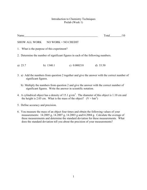
<strong>Introduction</strong> <strong>to</strong> <strong>Chemistry</strong> <strong>Techniques</strong><br />
<strong>Prelab</strong> (<strong>Week</strong> 1)<br />
Name___________________________________________________ Total________/10<br />
SHOW ALL WORK NO WORK = NO CREDIT<br />
1. What is the purpose of this experiment?<br />
2. Determine the number of significant figures in each of the following numbers.<br />
a) 23.7 b) 1340.1 c) 0.000218 d) 33.50<br />
3. a) Add the numbers from question 2 <strong>to</strong>gether and give the answer with the correct number of<br />
significant figures.<br />
b) Multiply the numbers from question 2 and give the answer with the correct number of<br />
significant figures. Write the answer in scientific notation.<br />
4. A cylindrical object has a density of 15.1 g/cm 3 . The diameter of this object is 1.10 cm and<br />
the height is 2.05 cm. What is the mass of the object? (V = hπr 2 )<br />
5. Define accuracy and precision.<br />
6. You measure the mass of an object four times and obtain the following values of your<br />
measurements: 14.2005 g, 14.2007 g, 14.2003 g and14.2004 g. Calculate the average of<br />
these measurements and determine the standard deviation for these measurements. What<br />
does the standard deviation tell you about the precision of your measurements?<br />
1
<strong>Introduction</strong> <strong>to</strong> <strong>Chemistry</strong> <strong>Techniques</strong><br />
<strong>Prelab</strong> (<strong>Week</strong> 2)<br />
Name___________________________________________________ Total________/10<br />
SHOW ALL WORK NO WORK = NO CREDIT<br />
1. The following graph shows absorbance versus concentration of a compound in solution.<br />
From the information on the graph given <strong>to</strong> you:<br />
Absorbance<br />
1.200<br />
1.000<br />
0.800<br />
0.600<br />
0.400<br />
0.200<br />
Absorbance vs. Concentration for nickel(II) sulfate hexaydrate<br />
y = 110.71x<br />
0.000<br />
0.00000 0.00100 0.00200 0.00300 0.00400 0.00500 0.00600 0.00700 0.00800 0.00900 0.01000<br />
concentration (mole/L)<br />
a) Determine the molar absorptivity (�) for this compound.<br />
b) Determine the concentration of an unknown solution that has an absorbance value of 0.567.<br />
Use the information given <strong>to</strong> you in the introduction.<br />
2
<strong>Introduction</strong> <strong>to</strong> <strong>Chemistry</strong> <strong>Techniques</strong><br />
In this experiment you will measure the mass of an object with two different kinds of balances<br />
and calculate the volume of liquid that is delivered from a transfer pipet. You will also<br />
determine the density of an object. The last part will introduce you <strong>to</strong> spectroscopy and how <strong>to</strong><br />
use absorbance of light <strong>to</strong> determine the concentration of an unknown solution.<br />
Special mention goes <strong>to</strong> Brian Stahl for developing Part IV of this labora<strong>to</strong>ry experiment <strong>to</strong> be<br />
used here in the Behrend chemistry curriculum.<br />
<strong>Introduction</strong><br />
Many experiments require some type of measurement, and are often simple measurements of<br />
mass and volume. The validity of an experiment is dependent on the reliability of these<br />
measurements. A measurement’s reliability is usually considered in terms of its precision.<br />
Precision is the closeness of the agreement between successive measurements of the same<br />
quantity. Precision is not <strong>to</strong> be confused with accuracy, the agreement of a particular value with<br />
the true value. The dispersion in a set of measurements is usually expressed in terms of the<br />
standard deviation, whose symbol is s. You are going <strong>to</strong> be asked <strong>to</strong> determine the standard<br />
deviation for some of your data. The standard deviation measures how close the data are<br />
clustered around the mean. The smaller the standard deviation, the more closely the data are<br />
clustered around the mean and the more precise your measurements are. After a quantity has<br />
been measured in an experiment, it may be necessary <strong>to</strong> use that measurement in a subsequent<br />
calculation. If you use a hand calcula<strong>to</strong>r for the arithmetic, eight or more digits may appear in<br />
the answer. It is up <strong>to</strong> you <strong>to</strong> decide how many of these digits are significant. IT IS YOUR<br />
RESPONSIBILITY TO KNOW THE RULES FOR SIGNIFICANT FIGURES BEFORE<br />
YOU START THIS EXPERIMENT.<br />
You will have <strong>to</strong> practice using an analytical and <strong>to</strong>p loader balance and then a transfer pipet so<br />
you can gain confidence <strong>to</strong> perform this experiment. Next, you will measure the mass of a flask<br />
four times on each balance. The precision of the measurements will be examined when you<br />
determine the correct number of significant figures in the mean mass of the flask. You will then<br />
add water <strong>to</strong> the flask from a filled 5-mL pipet, and then measure the mass of the flask and water.<br />
You will repeat this process three more times. After calculating the mass of the water that was<br />
delivered each time from the pipet, you will calculate the volume of each addition from the mass<br />
and density of water. You will then determine the correct number of significant figures in the<br />
mean volume. This number will allow you <strong>to</strong> appreciate the precision that you have achieved<br />
with the pipet.<br />
You will have <strong>to</strong> measure volume using a graduated cylinder. A graduated cylinder is used <strong>to</strong><br />
measure an approximate volume of a liquid. When water or an aqueous solution (a solution<br />
containing water) is added, the upper surface of the liquid in the graduated cylinder will be<br />
concave. This concave surface is called the meniscus. The bot<strong>to</strong>m of the meniscus is used for<br />
all measurements. To avoid error, your eye should always be level with the meniscus when you<br />
are measuring the volume. Using the graduated cylinder gives you the ability <strong>to</strong> measure the<br />
volume <strong>to</strong> only one decimal place.<br />
3
In the last part of this experiment, you will be using spectroscopy <strong>to</strong> determine the concentration<br />
of an unknown solution. There are many ways <strong>to</strong> determine concentrations of a substance in<br />
solution and using spectroscopy is only one method of determination. Many properties of a<br />
solution can change with concentration. The property you will be looking at in this experiment<br />
is colour. There is a direct correlation between colour intensity and concentration of a solution.<br />
Concentration and absorbance are linearly related. This means that the higher the concentration,<br />
the deeper the colour and therefore the higher the concentration of a substance in solution. The<br />
opposite is also true. Using colour can be much faster than using wet methods such as titration,<br />
especially when you have many samples containing different concentrations of the same<br />
substance. When coloured solutions are irradiated with white light, they will selectively absorb<br />
light of some wavelengths, but not of others. The wavelength at which absorbance is highest is<br />
the wavelength <strong>to</strong> which the solution is most sensitive <strong>to</strong> concentration changes. This<br />
wavelength is called the maximum wavelength or �max. In order <strong>to</strong> determine the precise amount<br />
of a substance present in a solution, a calibration curve must be produced. A calibration curve<br />
shows the relationship between the absorbance of light and the concentration of a chemical in a<br />
solution. The higher the concentration of a substance in solution, the deeper the colour will be<br />
and therefore the greater the absorbance of light. The opposite is also true. You will make four<br />
solutions where the concentration of your substance is known. By plotting the absorbance<br />
readings on the y-axis of the graph and the substance concentration values on the x-axis, you can<br />
use this information <strong>to</strong> determine the concentration of an unknown solution of that same<br />
substance. An example of a calibration plot is given. Once you have produced this calibration<br />
plot, you will then use it <strong>to</strong> determine the concentration of your unknown solution. The<br />
information you obtain from the calibration plot will be applied <strong>to</strong> Beer’s Law and the unknown<br />
concentration of your solution will be determined. The unit for concentration being used in this<br />
experiment is moles/litre.<br />
Beer’s law is defined by the following equation:<br />
A = �bc (1)<br />
The equation represents three variables that influence the response of a solution <strong>to</strong> light. They<br />
are the concentration (c) of the solution, the pathlength (b) of the light through the solution (also<br />
called the cell length) and the molar absorptivity (�), the sensitivity of the absorbing species at<br />
�max. The pathlength, unless it is stated differently, is usually fixed at 1.00 cm. The molar<br />
absorptivity value is dependent on the solvent used (in this case water) and �. The units for<br />
molar absorptivity are L/mole-cm for a concentration with units of mole/L.<br />
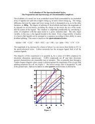
You will make four solutions where the concentration of your substance is known. By plotting<br />
the absorbance readings on the y-axis of the graph and the substance concentration values on the<br />
x-axis, you can use this information <strong>to</strong> determine the concentration of an unknown solution of<br />
that same substance. An example of a calibration plot is given. The slope of the line from the<br />
plot is the molar absorptivity for your chemical in solution. You will then measure the<br />
absorbance of a solution of unknown concentration. Using this absorbance value, along with the<br />
molar absorptivity determined from the calibration plot, you will be able <strong>to</strong> determine the<br />
concentration of your unknown solution by manipulating Beer’s Law:<br />
4
A<br />
c = (2)<br />
εb<br />
You will use pipets and volumetric flasks <strong>to</strong> make solutions of known concentrations as<br />
accurately as possible and measure the absorbance at �max. You will be making dilutions from a<br />
s<strong>to</strong>ck solution of a given substance. Since you will not be able <strong>to</strong> calculate dilutions yet, you will<br />
use the following equation <strong>to</strong> calculate your concentrations:<br />
C2 =<br />
C1xV<br />
V<br />
2<br />
where C1 is the concentration of your s<strong>to</strong>ck solution, V1 is the volume of the s<strong>to</strong>ck solution that<br />
you are measuring and V2 is the final volume of the solution. For example, if you measure five<br />
milliliters (mL) of your s<strong>to</strong>ck solution (V1) of known concentration (C1) and add it <strong>to</strong> a 100 mL<br />
volumetric flask and then added water <strong>to</strong> the line which indicated 100 mL of solution (V2), you<br />
could then find C2 using equation 3.<br />
FIGURE 1: A Calibration Curve of Copper(II) Sulphate Pentahydrate in Solution<br />
absorbance<br />
1.4<br />
1.2<br />
1<br />
0.8<br />
0.6<br />
0.4<br />
0.2<br />
1<br />
copper(II) sulphate pentahydrate<br />
0<br />
0 0.05 0.1 0.15 0.2 0.25 0.3 0.35<br />
concentration (moles/Litre)<br />
5<br />
(3)
Procedure<br />
Part I: Using the Balance<br />
1. Obtain about 100 mL of distilled water in a beaker. Allow the beaker and water <strong>to</strong> sit<br />
on the labora<strong>to</strong>ry bench while you are learning <strong>to</strong> use the balances and the pipet for parts II<br />
and III. The water should come <strong>to</strong> the temperature of the labora<strong>to</strong>ry during that time.<br />
2. Obtain a thermometer and a 50-mL Erlenmeyer flask with a rubber s<strong>to</strong>pper.<br />
3. Use the SAME <strong>to</strong>p loader balance throughout the experiment.<br />
4. Place the rubber s<strong>to</strong>pper in the Erlenmeyer flask. Tare the <strong>to</strong>p loader balance. Measure and<br />
record the combined masses of the flask and s<strong>to</strong>pper.<br />
5. Use tissue paper or paper <strong>to</strong>wel <strong>to</strong> remove the s<strong>to</strong>ppered flask from the pan of the balance.<br />
This is used because some balances are sensitive enough <strong>to</strong> detect the oils from your<br />
fingerprints and you will be weighing the flask on the analytical balance in step 9.<br />
6. Bring your balance <strong>to</strong> the zero position again. Measure and record the mass of the<br />
s<strong>to</strong>ppered flask once again.<br />
7. Repeat steps 5 and 6 until you have measured the mass four times.<br />
8. Calculate the mean (average) mass. The differences between the measured masses and the<br />
mean should be very small. If you are unsure of your results, consult your labora<strong>to</strong>ry<br />
instruc<strong>to</strong>r.<br />
9. Repeat steps 3-8 with the analytical balance. Be sure <strong>to</strong> use the SAME balance throughout<br />
the experiment.<br />
Part II: Using the Pipet<br />
Be sure <strong>to</strong> use the SAME BALANCE for ALL measurements.<br />
1. Obtain a 5 mL pipet.<br />
2. Practice using the pipet with distilled water (not the water you have set aside) until<br />
you are comfortable with the technique. You should plan on using the same analytical<br />
balance and the same pipet throughout the experiment.<br />
3. Using the thermometer, note the temperature of the labora<strong>to</strong>ry and of the distilled<br />
water that you have set aside. When the temperatures are identical or very nearly<br />
identical, you can begin. Record the temperature <strong>to</strong> the nearest degree.<br />
4. Measure and record the mass of the empty s<strong>to</strong>ppered flask again using the ANALYTICAL<br />
BALANCE. Use tissue paper/paper <strong>to</strong>wel as you did before.<br />
6
5. Remove the flask from the balance, using tissue paper. Pipet exactly 5 mL of the<br />
room-temperature water in<strong>to</strong> the flask without <strong>to</strong>uching the flask with your fingers.<br />
Using tissue paper/paper <strong>to</strong>wel, replace the s<strong>to</strong>pper <strong>to</strong> prevent evaporation.<br />
6. Bring your balance <strong>to</strong> the zero position. Measure and record the combined mass of the<br />
water and the s<strong>to</strong>ppered flask.<br />
7. Remove the flask from the balance. Do not pour out the first sample. Pipet another<br />
5 mL sample in<strong>to</strong> the flask. The volume of the water in the flask should now be 10 mL.<br />
Replace the s<strong>to</strong>pper and repeat step 6.<br />
8. Repeat until four samples of water have been delivered <strong>to</strong> the flask and the final<br />
volume is 20 mL.<br />
9. Calculate the mass of water that was delivered each time from your pipet. These<br />
masses should be approximately identical.<br />
10. Calculate the volume of each sample from the mass and density of water. Use Table 1<br />
<strong>to</strong> find the density that corresponds <strong>to</strong> your recorded temperature. Calculate the average<br />
volume delivered from each sample.<br />
Part III: Determining the Density of an Object<br />
1. Using your graduated cylinder, measure 40-50 mL of water from your beaker in Part I and<br />
leave it in the graduated cylinder. Record this measurement <strong>to</strong> the nearest 0.1 mL.<br />
2. Take one of the objects from the samples that are given and find its mass on the<br />
analytical balance.<br />
3. Place that same object in the graduated cylinder with the water in it. Make sure that<br />
the object is completely submerged in the water. If the object is not completely<br />
submerged, repeat steps 1and 2 being sure <strong>to</strong> dry the object and adding more water in<br />
the graduated cylinder. Avoid splashing any water out of the graduated cylinder or cracking<br />
the bot<strong>to</strong>m of the graduated cylinder.<br />
4. Record the level of the water with object in the graduated cylinder. The difference<br />
between this measurement and the measurement in step 1 is the volume of the object.<br />
5. Using the same object that has been dried well, measure the width and height of the object <strong>to</strong><br />
the nearest 0.01 cm.<br />
6. Calculate the volume of the object using the measurements determined in step 5.<br />
7. Calculate the density of the object (g/mL and g/cm 3 using the volumes from step 4 and step 6)<br />
using the correct number of significant figures.<br />
7
Table 1 Density (g/mL) of Water at Various Temperatures ( o C)<br />
Temp. Density Temp. Density Temp. Density<br />
17 0.9988 22 0.9978 27 0.9965<br />
18 0.9986 23 0.9976 28 0.9962<br />
19 0.9984 24 0.9973 29 0.9959<br />
20 0.9982 25 0.9971 30 0.9956<br />
21 0.9980 26 0.9968 31 0.9953<br />
Example I: How <strong>to</strong> Calculate a Standard Deviation<br />
You obtain the following measurements: 15.2654, 15.2657, 15.2658 and 15.2655. In the<br />
following calculations, each individual measurement from above will be represented using the<br />
symbol xi and the mean (the average of these values) will be given the symbol x .<br />
2<br />
d i<br />
s �<br />
N �1<br />
�<br />
� means “the sum of”<br />
di = xi - x<br />
N = the number of measurements<br />
x = 15.2656<br />
xi di (xi – x ) di 2<br />
15.2654 -0.0002 0.00000004<br />
15.2657 0.0001 0.00000001<br />
15.2658 0.0002 0.00000004<br />
15.2655 -0.0001 0.00000001<br />
0.00000010 = � di 2<br />
0.00000010<br />
s � = 0.000183 = 0.0002<br />
4 �1<br />
When you report a value, it is the mean (average) value that is reported along with the standard<br />
deviation <strong>to</strong> show the precision of the measurements which contributed <strong>to</strong> the mean value.<br />
Therefore, the value reported for this example would be 15.2656 � 0.0002.<br />
8
Part IV: Using Spectroscopy <strong>to</strong> Determine the Concentration of an Unknown Solution<br />
1. Using a 250.0 mL beaker, obtain approximately 75.0 mL of s<strong>to</strong>ck solution of known<br />
concentration (write this concentration down).<br />
2. Using a pipet, transfer 5.0 mL of s<strong>to</strong>ck solution <strong>to</strong> a 100.0 mL volumetric flask and<br />
fill up <strong>to</strong> the 100.0 mL mark with distilled water. Mix and then transfer all the solution <strong>to</strong> a<br />
clean dry beaker that is 150 mL or greater. This will be called solution 2.<br />
3. You will do this three more times making solution 3 (10.0 mL of s<strong>to</strong>ck solution diluted <strong>to</strong><br />
100.0 mL), solution 4 (15.0 mL of s<strong>to</strong>ck solution diluted <strong>to</strong> 100.0 mL), and solution 5 (20.0<br />
mL of s<strong>to</strong>ck solution diluted <strong>to</strong> 100.0 mL). Remember, all dilutions are made with distilled<br />
water and remember <strong>to</strong> place each solution in a beaker after mixing. Calculate the<br />
concentrations (C2) of solutions 2-5 using equation 3 on page 5. You will need these values<br />
when you make your calibration plot.<br />
4. Once all your solutions are made and concentrations have been calculated, go <strong>to</strong> the netbook<br />
and open up the Chem 111 folder. Select the file labeled “<strong>Introduction</strong> <strong>to</strong> <strong>Chemistry</strong><br />
<strong>Techniques</strong> Fall 2011” and double click on that file. You will then see a table and a graph on<br />
the screen.<br />
5. Take distilled water and pour it in the cuvette. Make sure there are no fingerprints and that<br />
the light is passing through the smooth surfaces not the ribbed surfaces. Fill cuvette with<br />
distilled water <strong>to</strong> make a blank.<br />
6. On the menu bar, select Experiment, then Calibrate, and then Spectrometer:1. Wait for the<br />
lamp <strong>to</strong> warm up.<br />
7. When the lamp has warmed up, place the blank in the spectrometer. Click Finish<br />
Calibration, then click OK. Keep the blank in the spectrometer since this will be your first<br />
data point.<br />
8. In the <strong>to</strong>p right hand corner, you will see the collect icon . Click on collect.<br />
You should see a very low absorbance value in the bot<strong>to</strong>m left hand corner of the screen. If<br />
you do not have a very low value, get help from your instruc<strong>to</strong>r. Once you have waited 20-30<br />
seconds, go <strong>to</strong> the <strong>to</strong>p right hand corner of the screen where it says keep and click.<br />
You will now be asked for the concentration. Since this is your blank, the concentration is<br />
zero.<br />
9. Repeat step 8 for the rest of the solutions. Remember <strong>to</strong> wait 20-30 seconds before clicking<br />
on keep. Copy all the absorbance values as well as the respective concentrations in your<br />
labora<strong>to</strong>ry notebook.<br />
9
10. When you are all done getting the absorbances for solutions 2-5, click on the s<strong>to</strong>p icon.<br />
Then go <strong>to</strong> the linear fit icon and click. A box filled with information will appear and<br />
you will find the value of the slope of the graph (m). This is your molar absorptivity value.<br />
Record that value.<br />
11. You will now take a sample of an unknown solution and place it in a clean cuvette. Place<br />
the cuvette in the spectrometer and read the absorbance value for that solution from the<br />
netbook. Now you can calculate the concentration of your unknown solution by using<br />
equation 2.<br />
Results<br />
Part I<br />
Using the Analytical Balance<br />
Mass of the s<strong>to</strong>ppered<br />
flask (g) ____________ ____________ ____________ ____________<br />
Calculation:<br />
Using the Top Loader Balance<br />
Mean mass (g) ____________<br />
Mass of the s<strong>to</strong>ppered<br />
flask (g) ____________ ____________ ____________ ____________<br />
Mean mass (g) ____________<br />
10
Part II<br />
Using the Pipet<br />
Temperature ( o C) __________ Density of water (g/mL) __________<br />
Addition No. 1 2 3 4<br />
Mass after<br />
addition (g) __________ __________ __________ __________<br />
Mass before<br />
addition (g) __________ __________ __________ __________<br />
Mass of water<br />
in flask (g) __________ __________ __________ __________<br />
Volume of water<br />
delivered each<br />
time (mL) __________ __________ __________ __________<br />
Mean volume (mL) __________<br />
Calculations (One sample calculation for one addition in Part II):<br />
Part III<br />
Determining the Density of an Object<br />
Mass of the object (g) __________<br />
Volume after adding object (mL) __________<br />
Volume before adding object (mL) __________ Volume of object (mL) __________<br />
Diameter of object (cm) ____________ Volume of object (cm 3 ) __________<br />
(using the equation V = h�r 2 )<br />
Radius of object (cm) __________<br />
Height of object (cm) __________<br />
Density of the object (g/mL) __________<br />
Density of the object (g/cm 3 ) ____________<br />
Calculations:<br />
11
Part IV<br />
Solution Concentration Absorbance<br />
1 0.000 0.00<br />
2<br />
3<br />
4<br />
5<br />
Unknown ?<br />
Unknown Letter or Number ________<br />
Concentration of S<strong>to</strong>ck Solution __________________<br />
Molar Absorptivity of Chemical in Solution __________________<br />
Concentration of Unknown Solution____________________<br />
Calcuations:<br />
Questions<br />
1 a. Calculate the standard deviation (look at example on page 8) for the volume of water<br />
delivered each time in Part II.<br />
b. What does the standard deviation from part a tell you about the precision of your<br />
measurements?<br />
12