Experiment 1: Colligative Properties
Experiment 1: Colligative Properties
Experiment 1: Colligative Properties

Create successful ePaper yourself
Turn your PDF publications into a flip-book with our unique Google optimized e-Paper software.
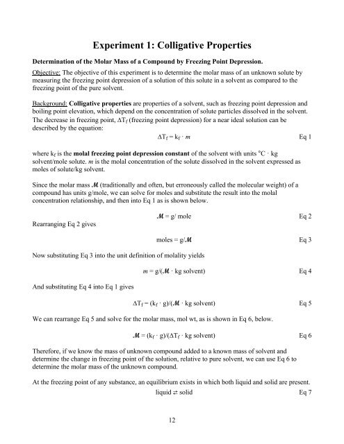
<strong>Experiment</strong> 1: <strong>Colligative</strong> <strong>Properties</strong><br />
Determination of the Molar Mass of a Compound by Freezing Point Depression.<br />
Objective: The objective of this experiment is to determine the molar mass of an unknown solute by<br />
measuring the freezing point depression of a solution of this solute in a solvent as compared to the<br />
freezing point of the pure solvent.<br />
Background: <strong>Colligative</strong> properties are properties of a solvent, such as freezing point depression and<br />
boiling point elevation, which depend on the concentration of solute particles dissolved in the solvent.<br />
The decrease in freezing point, ΔTf (freezing point depression) for a near ideal solution can be<br />
described by the equation:<br />
ΔTf = kf · m Eq 1<br />
where kf is the molal freezing point depression constant of the solvent with units °C · kg<br />
solvent/mole solute. m is the molal concentration of the solute dissolved in the solvent expressed as<br />
moles of solute/kg solvent.<br />
Since the molar mass M (traditionally and often, but erroneously called the molecular weight) of a<br />
compound has units g/mole, we can solve for moles and substitute the result into the molal<br />
concentration relationship, and then into Eq 1 as is shown below.<br />
Rearranging Eq 2 gives<br />
Now substituting Eq 3 into the unit definition of molality yields<br />
And substituting Eq 4 into Eq 1 gives<br />
M = g/ mole Eq 2<br />
moles = g/M Eq 3<br />
m = g/(M · kg solvent) Eq 4<br />
ΔTf = (kf · g)/(M · kg solvent) Eq 5<br />
We can rearrange Eq 5 and solve for the molar mass, mol wt, as is shown in Eq 6, below.<br />
M = (kf · g)/(ΔTf · kg solvent) Eq 6<br />
Therefore, if we know the mass of unknown compound added to a known mass of solvent and<br />
determine the change in freezing point of the solution, relative to pure solvent, we can use Eq 6 to<br />
determine the molar mass of the unknown compound.<br />
At the freezing point of any substance, an equilibrium exists in which both liquid and solid are present.<br />
liquid ⇄ solid Eq 7<br />
12
The temperature at which this equilibrium exists is the freezing point of the substance. Sometimes this<br />
temperature is difficult to determine, so the use of cooling curves is required. To construct a cooling<br />
curve one would warm their sample, pure solvent or solution, to well above its melting point, then<br />
allow it to cool. As the sample cools the temperature of the sample is monitored as a function of time.<br />
As the sample begins to solidify the change in temperature will slow, and at the equilibrium shown by<br />
Eq 7 the temperature will be constant until all of the sample has solidified. A graph is made by plotting<br />
the temperature vs. time. An example of a cooling curve is shown below in Figure 1.<br />
Temp, C<br />
70<br />
65<br />
60<br />
55<br />
50<br />
45<br />
40<br />
35<br />
30<br />
0 20 40 60 80 100<br />
time, s<br />
Figure 1: Cooling curve for a pure solvent.<br />
In this cooling curve you see a steady decrease in temperature followed by a dip which is followed by<br />
a slight rise in the temperature. This dip is not unusual and results from supercooling during the early<br />
stages of the freezing process. In this example the dip is followed by a short plateau in the temperature.<br />
This plateau is at the freezing point of the pure solvent as shown in Figure 1.<br />
When solute is added to the solvent the shape of the cooling curve sometimes changes so that we don’t<br />
see a clear horizontal plateau as the example shown in Figure 1.<br />
Temp, C<br />
70<br />
65<br />
60<br />
55<br />
50<br />
45<br />
40<br />
35<br />
30<br />
25<br />
20<br />
0 20 40 60 80 100<br />
time, s<br />
Figure 2: Cooling curve for a solution.<br />
13
In Figure 2 we don’t see a clear horizontal plateau. In this case we must draw a trend line through the<br />
data points corresponding to the cooling of the liquid and a trend line through the data points<br />
corresponding to the freezing of the liquid. The temperature at the point where those two lines intersect<br />
is the freezing point of the solution.<br />
Temp, o C<br />
70<br />
65<br />
60<br />
55<br />
50<br />
45<br />
40<br />
35<br />
30<br />
0 20 40 60 80 100<br />
time, s<br />
Figure 3: Solution cooling curve<br />
showing best fit straight lines through the two portions<br />
of the curve discussed in the text.<br />
Figure 3 shows an example with the trend lines drawn in and the intersection of the lines. In the<br />
example shown in Figure 3 the freezing point would be measured as about 43 °C. If we continue to<br />
record and plot the temperature of the solid, the data points may start to deviate from the trend line<br />
shown in Figure 3 corresponding to the freezing of the liquid. In this case you would not include those<br />
points in the trend line.<br />
In this experiment you will determine the freezing point of pure tertiary butyl alcohol (t-butanol) then<br />
the freezing point of t-butanol with an unknown solute dissolved in it. From these freezing point<br />
measurements you will be able to calculate the molar mass of the unknown solute. The t-butanol is a<br />
good solvent choice for this experiment. Its transition state from solid to liquid occurs near room<br />
temperature, so it has a relatively low melting point, thus a low freezing point. It also has a relatively<br />
large kf, 9.10 ºC·kg solvent/mol solute, which is good for estimating the molar mass of a solute<br />
because it will allow us to see a greater ΔTf relative to a solvent with a lower kf.<br />
Procedure: For this experiment you will need a 150 ml beaker, two 400 ml beakers, a large test tube<br />
(25 x 150 mm), a tripod stand with wire mess, a thermometer, a stirring loop and a Bunsen burner.<br />
Freezing point of pure t-butanol:<br />
Place a 150 ml beaker on a top loader balance and tare it. Place a clean, dry 25 x 150 mm test tube in<br />
the beaker and record the mass in the data table, line 1. Fill the test tube about half full with t-butanol,<br />
reweigh and record this mass in the data table, line 2. Place the beaker and test tube aside for now.<br />
Place about 250 ml of hot tap water in one 400 ml beaker and place the test tube containing the tbutanol<br />
in the hot water; we want to warm the t-butanol to about 40 °C. You may use a tripod and<br />
Bunsen burner to warm the t-butanol in the water bath if needed. (Do not heat the test tube with a<br />
14
direct flame!) Insert the stirring loop into the test tube and then insert the thermometer so that the loop<br />
of the stirrer surrounds the thermometer. Periodically stir the t-butanol with the stirring loop by an up<br />
and down motion while warming it.<br />
Place about 250-300 ml of ice in the other 400 ml beaker and enough cold tap water to just cover the<br />
ice. Once the temperature of the t-butanol has warmed to about 40 °C, transfer the test tube to the icewater<br />
bath making sure that most of the t-butanol is below the surface of the ice-water bath, add more<br />
ice if needed. Immediately begin to take temperature readings and record them in the table every 15<br />
seconds while continually stirring the t-butanol with the stirring loop in an up and down motion.<br />
Continue to stir and take temperature readings every 15 seconds until the t-butanol has solidified.<br />
When the t-butanol has solidified so that the stirring loop will no longer move, stop trying to stir, but<br />
continue to record the temperature every 15 seconds for one more minute. Do not try to pull the<br />
thermometer and stirrer from the frozen t-butanol! Doing so may break the thermometer.<br />
Freezing point of solutions:<br />
Place the test tube in the 150 ml beaker, the test tube may now be top heavy, so use caution, or use a<br />
250 ml beaker. Place the beaker with test tube on a top loader balance and tare the balance. With a<br />
disposable pipette add about 0.5 g of our unknown to the test tube and record the mass, line 4. Reheat<br />
the test tube as before to about 40 °C, this is sample solution 1. If you need fresh hot tap water in<br />
which to warm your sample, get it. Try to make sure all your unknown is dissolved in the t-butanol.<br />
Use the stirring loop to aid the dissolution of the solute, if needed. If you need more ice for your icewater<br />
bath get it. As before, once the temperature is about 40 °C, transfer the test tube to the ice-water<br />
bath. Begin stirring and take temperature readings every 15 seconds until the solution has solidified.<br />
When the solution has solidified so that you can no longer stir it, stop trying to stir, but continue to<br />
record the temperature every 15 seconds for one more minute.<br />
Return the test tube to the 150 ml beaker and place the beaker with test tube on a top loader balance<br />
and tare the balance. With a disposable pipette add about another 0.5 g of the unknown to the test tube<br />
and record the mass, line 5 (this is sample solution 2). Repeat the melting and temperature recording<br />
steps outlined in the previous paragraph.<br />
Clean-Up: Place the test tube back in the warm water bath to melt the solid. Remove the thermometer<br />
and stirring loop. Pour the t-butanol solutions into the waste beaker under the fume hood. Wash the<br />
thermometer, stirring loop and test tube in the sink with soap and water, dry and return them to the side<br />
shelf. Empty all beakers and other glassware you used and return them to your drawer.<br />
15
Data:<br />
1) Mass of test tube:<br />
2) Mass of test tube and t-butanol:<br />
3) a) Mass of t-butanol (line 2 – line 1):<br />
b) Mass of t-butanol in kgs:<br />
4) Mass of first sample of unknown:<br />
5) Mass of second sample of unknown:<br />
6) Total mass of unknown in second solution freezing point<br />
determination (line 4 + line 5):<br />
16
Data Table:<br />
t-butanol,<br />
t-butanol plus first sample t-butanol plus second sample<br />
pure solvent<br />
portion, solution 1<br />
portion, solution 2<br />
time temperature time temperature time temperature<br />
17
Data Handling, Calculations and Questions:<br />
Use graph paper and plot temperature vs. time for the pure t-butanol and for each solution analyzed;<br />
make 3 different graphs. Use the discussion in the background section above as a guide and determine<br />
the freezing point, Tf, of t-butanol and of each solution. Clearly mark on each graph all your data<br />
points and the best fit lines you used to determine each freezing point. Determine the ΔTf of solution 1<br />
by subtracting the Tf of solution 1 from the Tf of pure t-butanol. Determine the ΔTf of solution 2 by<br />
subtracting the Tf of solution 2 from the Tf of pure t-butanol.<br />
Use the ΔTf for solution 1 along with the mass of unknown in solution 1, line 4 of the data table, the<br />
mass of solvent, t-butanol, line 3b of the data table, and the kf of t-butanol, 9.10 ºC·kg solvent/mol<br />
solute, in Eq 6 to determine the molar mass, M, of your unknown compound.<br />
Repeat the calculation above for solution 2 remembering to use the total mass of solute, line 6 of the<br />
data table, and the ΔTf for solution 2.<br />
Report:<br />
In your lab report briefly discuss the theory behind why the freezing point of a solution is typically<br />
lower than the freezing point of pure solvent.<br />
Reproduce the data from the Data page and the Data Table, pages 5 and 6, and turn in with your report,<br />
along with all three graphs.<br />
Make a data and calculations page to report the Tf of pure t-butanol and for each solution. Show all<br />
calculations and report the molar mass of unknown as determined in each of the two solutions.<br />
Average the two molar masses you determined and calculate the percent difference for each<br />
determination vs. the average. This should give you about a 6 or 7 page lab report, not all pages will be<br />
full of text.<br />
Reference:<br />
Some information at the following lab experiment was used for this experiment.<br />
http://infohost.nmt.edu/~jaltig/FreezingPtDep.pdf<br />
18