Benders decomposition with gams - Amsterdam Optimization ...
Benders decomposition with gams - Amsterdam Optimization ...
Benders decomposition with gams - Amsterdam Optimization ...

Create successful ePaper yourself
Turn your PDF publications into a flip-book with our unique Google optimized e-Paper software.
BENDERS DECOMPOSITION WITH GAMS<br />
ERWIN KALVELAGEN<br />
Abstract. This document describes an implementation of <strong>Benders</strong> Decomposition<br />
using GAMS.<br />
1. Introduction<br />
<strong>Benders</strong>’ Decomposition[2] is a popular technique in solving certain classes of difficult<br />
problems such as stochastic programming problems[7, 13] and mixed-integer<br />
nonlinear programming problems[6, 5]. In this document we describe how a <strong>Benders</strong>’<br />
Decomposition algorithm for a MIP problem can be implemented in a GAMS<br />
environment. For stochastic programming examples of <strong>Benders</strong>’ Decomposition<br />
implemented in GAMS see [9, 11]. For a simple generalized <strong>Benders</strong>’ model for an<br />
MINLP model see [10].<br />
(1)<br />
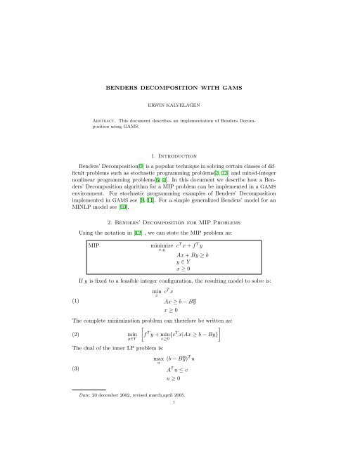
2. <strong>Benders</strong>’ Decomposition for MIP Problems<br />
Using the notation in [12] , we can state the MIP problem as:<br />
MIP minimize<br />
x,y<br />
c T x + f T y<br />
Ax + By ≥ b<br />
y ∈ Y<br />
x ≥ 0<br />
If y is fixed to a feasible integer configuration, the resulting model to solve is:<br />
min<br />
x<br />
c T x<br />
Ax ≥ b − By<br />
x ≥ 0<br />
The complete minimization problem can therefore be written as:<br />
�<br />
(2) min<br />
y∈Y<br />
f T y + min<br />
x≥0 {cT �<br />
x|Ax ≥ b − By}<br />
The dual of the inner LP problem is:<br />
(3)<br />
max<br />
u<br />
(b − By) T u<br />
A T u ≤ c<br />
u ≥ 0<br />
Date: 20 december 2002, revised march,april 2005.<br />
1
2 ERWIN KALVELAGEN<br />
In the <strong>Benders</strong>’ <strong>decomposition</strong> framework two different problems are solved. A<br />
restricted master problem which has the form:<br />
(4)<br />
min<br />
y<br />
z<br />
z ≥ f T y + (b − By) T uk, k = 1, . . . , K<br />
(b − By) T uℓ ≤ 0, ℓ = 1, . . . , L<br />
y ∈ Y<br />
and subproblems of the form:<br />
(5)<br />
max<br />
u<br />
f T y + (b − By) T u<br />
A T u ≤ c<br />
u ≥ 0<br />
The <strong>Benders</strong>’ Decomposition algorithm can be stated as:<br />
{initialization}<br />
y := initial feasible integer solution<br />
LB := −∞<br />
UB := ∞<br />
while UB − LB > ɛ do<br />
{solve subproblem}<br />
maxu{f T y + (b − By) T u|A T u ≤ c, u ≥ 0}<br />
if Unbounded then<br />
Get unbounded ray u<br />
Add cut (b − By) T u ≤ 0 to master problem<br />
else<br />
Get extreme point u<br />
Add cut z ≥ f T y + (b − By) T u to master problem<br />
UB := min{UB, f T y + (b − By) T u}<br />
end if<br />
{solve master problem}<br />
miny{z|cuts, y ∈ Y }<br />
LB := z<br />
end while<br />
The subproblem is a dual LP problem, and the master problem is a pure IP<br />
problem (no continuous variables are involved). <strong>Benders</strong>’ Decomposition for MIP<br />
is of special interest when the <strong>Benders</strong>’ subproblem and the relaxed master problem<br />
are easy to solve, while the original problem is not.<br />
3. The Fixed Charge Transportation Problem<br />
The problem we consider is the Fixed Charge Transportation Problem (FCTP)[1,<br />
14]. The standard transportation problem can be described as:
TP minimize<br />
x<br />
�<br />
ci,jxi,j<br />
�i,j<br />
xi,j = si<br />
�j<br />
xi,j = dj<br />
i<br />
xi,j ≥ 0<br />
The fixed charge transportation problem adds a fixed cost fi,j to a link i → j.<br />
This can be modeled using extra binary variables yi,j indicating whether a link is<br />
open or closed:<br />
FCTP minimize<br />
x,y<br />
�<br />
(fi,jyi,j + ci,jxi,j)<br />
�i,j<br />
xi,j = si<br />
�j<br />
xi,j = dj<br />
i<br />
xi,j ≤ Mi,jyi,j<br />
xi,j ≥ 0, yi,j ∈ {0, 1}<br />
where Mi,j are large enough numbers. When solving this as a straight MIP problem,<br />
it is important to assign reasonable values to Mi,j. As Mi,j can be considered as<br />
an upper bound on xi,j, we can find good values:<br />
(6) Mi,j = min{si, dj}<br />
(7)<br />
When we rewrite the problem as<br />
�<br />
min ci,jxi,j +<br />
x,y<br />
i,j<br />
�<br />
i,j<br />
− �<br />
xi,j ≥ −si<br />
�<br />
i<br />
j<br />
xi,j ≥ dj<br />
fi,jyi,j<br />
− xi,j + Mi,jyi,j ≥ 0<br />
xi,j ≥ 0<br />
yi,j ∈ {0, 1}<br />
we see that the <strong>Benders</strong>’ subproblem can be stated as:<br />
�<br />
max (−si)ui +<br />
u,v,w<br />
i<br />
�<br />
djvj +<br />
j<br />
�<br />
i,j<br />
(8)<br />
− ui + vj − wi,j ≤ ci,j<br />
ui ≥ 0, vj ≥ 0, wi,j ≥ 0<br />
(−Mi,jy i,j)wi,j<br />
3
4 ERWIN KALVELAGEN<br />
(9)<br />
The <strong>Benders</strong>’ Relaxed Master Problem can be written as:<br />
min z<br />
y<br />
z ≥ �<br />
fi,jyi,j + �<br />
(−si)u (k)<br />
� �<br />
+ +<br />
�<br />
i<br />
i,j<br />
(−si)u (ℓ)<br />
i<br />
yi,j ∈ {0, 1}<br />
+ �<br />
j<br />
i<br />
djv (ℓ)<br />
j<br />
i<br />
+ �<br />
j<br />
djv (k)<br />
j<br />
(−Mi,jw<br />
i,j<br />
(ℓ)<br />
i,j )yi,j ≤ 0<br />
Using this result the GAMS model can now be formulated as:<br />
Model benders.gms. 1<br />
$ontext<br />
An example of <strong>Benders</strong> Decomposition on fixed charge transportation<br />
problem bk4x3.<br />
Optimal objective in reference : 350.<br />
Erwin Kalvelagen, December 2002<br />
See:<br />
http://www.in.tu-clausthal.de/~gottlieb/benchmarks/fctp/<br />
http://www.<strong>gams</strong>.com/~erwin/benders/benders.pdf<br />
$offtext<br />
set i ’sources’ /i1*i4/;<br />
set j ’demands’ /j1*j3/;<br />
parameter supply(i) /<br />
i1 10<br />
i2 30<br />
i3 40<br />
i4 20<br />
/;<br />
parameter demand(j) /<br />
j1 20<br />
j2 50<br />
j3 30<br />
/;<br />
table c(i,j) ’variable cost’<br />
j1 j2 j3<br />
i1 2.0 3.0 4.0<br />
i2 3.0 2.0 1.0<br />
i3 1.0 4.0 3.0<br />
i4 4.0 5.0 2.0<br />
;<br />
table f(i,j) ’fixed cost’<br />
j1 j2 j3<br />
i1 10.0 30.0 20.0<br />
i2 10.0 30.0 20.0<br />
i3 10.0 30.0 20.0<br />
i4 10.0 30.0 20.0<br />
;<br />
*<br />
1 http://www.amsterdamoptimization.com/models/benders/benders.gms<br />
(−Mi,jw<br />
i,j<br />
(k)<br />
i,j )yi,j
* check supply-demand balance<br />
*<br />
scalar totdemand, totsupply;<br />
totdemand = sum(j, demand(j));<br />
totsupply = sum(i, supply(i));<br />
abort$(abs(totdemand-totsupply)>0.001) "Supply does not equal demand.";<br />
*<br />
* for big-M formulation we need tightest possible upperbounds on x<br />
*<br />
parameter xup(i,j) ’tight upperbounds for x(i,j)’;<br />
xup(i,j) = min(supply(i),demand(j));<br />
*--------------------------------------------------------------------<br />
* standard MIP problem formulation<br />
*--------------------------------------------------------------------<br />
variables<br />
cost ’objective variable’<br />
x(i,j) ’shipments’<br />
y(i,j) ’on-off indicator for link’<br />
;<br />
positive variable x;<br />
binary variable y;<br />
equations<br />
obj ’objective’<br />
cap(i) ’capacity constraint’<br />
dem(j) ’demand equation’<br />
xy(i,j) ’y=0 => x=0’<br />
;<br />
obj.. cost =e= sum((i,j), f(i,j)*y(i,j) + c(i,j)*x(i,j));<br />
cap(i).. sum(j, x(i,j)) =l= supply(i);<br />
dem(j).. sum(i, x(i,j)) =g= demand(j);<br />
xy(i,j).. x(i,j) =l= xup(i,j)*y(i,j);<br />
display "--------------------- standard MIP formulation----------------------";<br />
option optcr=0;<br />
option limrow=0;<br />
option limcol=0;<br />
model fscp /obj,cap,dem,xy/;<br />
solve fscp minimizing cost using mip;<br />
*---------------------------------------------------------------------<br />
* <strong>Benders</strong> Decomposition Initialization<br />
*---------------------------------------------------------------------<br />
display "--------------------- BENDERS ALGORITHM ----------------------------";<br />
scalar UB ’upperbound’ /INF/;<br />
scalar LB ’lowerbound’ /-INF/;<br />
y.l(i,j) = 1;<br />
*---------------------------------------------------------------------<br />
* <strong>Benders</strong> Subproblem<br />
*---------------------------------------------------------------------<br />
variable z ’objective variable’;<br />
positive variables<br />
u(i) ’duals for capacity constraint’<br />
v(j) ’duals for demand constraint’<br />
w(i,j) ’duals for xy constraint’<br />
;<br />
equations<br />
subobj ’objective’<br />
5
6 ERWIN KALVELAGEN<br />
;<br />
subconstr(i,j) ’dual constraint’<br />
* to detect unbounded subproblem<br />
scalar unbounded /1.0e6/;<br />
z.up = unbounded;<br />
subobj.. z =e= sum(i, -supply(i)*u(i)) + sum(j, demand(j)*v(j))<br />
+ sum((i,j), -xup(i,j)*y.l(i,j)*w(i,j))<br />
;<br />
subconstr(i,j).. -u(i) + v(j) - w(i,j) =l= c(i,j);<br />
model subproblem /subobj, subconstr/;<br />
* reduce output to listing file:<br />
subproblem.solprint=2;<br />
* speed up by keeping GAMS in memory:<br />
subproblem.solvelink=2;<br />
*---------------------------------------------------------------------<br />
* <strong>Benders</strong> Modified Subproblem to find unbounded ray<br />
*---------------------------------------------------------------------<br />
variable dummy ’dummy objective variable’;<br />
equations<br />
modifiedsubobj ’objective’<br />
modifiedsubconstr(i,j) ’dual constraint’<br />
edummy;<br />
;<br />
modifiedsubobj..<br />
sum(i, -supply(i)*u(i)) + sum(j, demand(j)*v(j))<br />
+ sum((i,j), -xup(i,j)*y.l(i,j)*w(i,j)) =e= 1;<br />
modifiedsubconstr(i,j)..<br />
-u(i) + v(j) - w(i,j) =l= 0;<br />
edummy.. dummy =e= 0;<br />
model modifiedsubproblem /modifiedsubobj, modifiedsubconstr, edummy/;<br />
* reduce output to listing file:<br />
modifiedsubproblem.solprint=2;<br />
* speed up by keeping GAMS in memory:<br />
modifiedsubproblem.solvelink=2;<br />
*---------------------------------------------------------------------<br />
* <strong>Benders</strong> Relaxed Master Problem<br />
*---------------------------------------------------------------------<br />
set iter /iter1*iter50/;<br />
set cutset(iter) ’dynamic set’;<br />
cutset(iter)=no;<br />
set unbcutset(iter) ’dynamic set’;<br />
unbcutset(iter)=no;<br />
variable z0 ’relaxed master objective variable’;<br />
equations<br />
cut(iter) ’<strong>Benders</strong> cut for optimal subproblem’<br />
unboundedcut(iter) ’<strong>Benders</strong> cut for unbounded subproblem’<br />
;<br />
parameters<br />
cutconst(iter) ’constant term in cuts’<br />
cutcoeff(iter,i,j)<br />
;<br />
cut(cutset).. z0 =g= sum((i,j), f(i,j)*y(i,j))<br />
+ cutconst(cutset)
+ sum((i,j), cutcoeff(cutset,i,j)*y(i,j));<br />
unboundedcut(unbcutset)..<br />
cutconst(unbcutset)<br />
+ sum((i,j), cutcoeff(unbcutset,i,j)*y(i,j)) =l= 0;<br />
model master /cut,unboundedcut/;<br />
* reduce output to listing file:<br />
master.solprint=2;<br />
* speed up by keeping GAMS in memory:<br />
master.solvelink=2;<br />
* solve to optimality<br />
master.optcr=0;<br />
*---------------------------------------------------------------------<br />
* <strong>Benders</strong> Algorithm<br />
*---------------------------------------------------------------------<br />
scalar converged /0/;<br />
scalar iteration;<br />
scalar bound;<br />
parameter ybest(i,j);<br />
parameter log(iter,*) ’logging info’;<br />
loop(iter$(not converged),<br />
*<br />
* solve <strong>Benders</strong> subproblem<br />
*<br />
solve subproblem maximizing z using lp;<br />
*<br />
* check results.<br />
*<br />
abort$(subproblem.modelstat>=2) "Subproblem not solved to optimality";<br />
*<br />
* was subproblem unbounded?<br />
*<br />
if (z.l+1 < unbounded,<br />
*<br />
* no, so update upperbound<br />
*<br />
bound = sum((i,j), f(i,j)*y.l(i,j)) + z.l;<br />
if (bound < UB,<br />
UB = bound;<br />
ybest(i,j) = y.l(i,j);<br />
display ybest;<br />
);<br />
*<br />
* and add <strong>Benders</strong>’ cut to Relaxed Master<br />
*<br />
cutset(iter) = yes;<br />
else<br />
*<br />
* solve modified subproblem<br />
*<br />
solve modifiedsubproblem maximizing dummy using lp;<br />
*<br />
* check results.<br />
*<br />
7
8 ERWIN KALVELAGEN<br />
abort$(modifiedsubproblem.modelstat>=2)<br />
"Modified subproblem not solved to optimality";<br />
*<br />
* and add <strong>Benders</strong>’ cut to Relaxed Master<br />
*<br />
unbcutset(iter) = yes;<br />
);<br />
*<br />
* cut data<br />
*<br />
cutconst(iter) = sum(i, -supply(i)*u.l(i)) + sum(j, demand(j)*v.l(j));<br />
cutcoeff(iter,i,j) = -xup(i,j)*w.l(i,j);<br />
*<br />
* solve Relaxed Master Problem<br />
*<br />
option optcr=0;<br />
solve master minimizing z0 using mip;<br />
*<br />
* check results.<br />
*<br />
abort$(master.modelstat=4) "Relaxed Master is infeasible";<br />
abort$(master.modelstat>=2) "Masterproblem not solved to optimality";<br />
*<br />
* update lowerbound<br />
*<br />
);<br />
LB = z0.l;<br />
log(iter,’LB’) = LB;<br />
log(iter,’UB’) = UB;<br />
iteration = ord(iter);<br />
display iteration,LB,UB;<br />
converged$( (UB-LB) < 0.1 ) = 1;<br />
display$converged "Converged";<br />
display log;<br />
abort$(not converged) "No convergence";<br />
*<br />
* recover solution<br />
*<br />
y.fx(i,j) = ybest(i,j);<br />
fscp.solvelink=2;<br />
fscp.solprint=2;<br />
solve fscp minimizing cost using rmip;<br />
abort$(fscp.modelstat1) "final lp not solved to optimality";<br />
display "<strong>Benders</strong> solution",y.l,x.l,cost.l;<br />
The <strong>Benders</strong>’ algorithm will converge to the optimal solution in 17 cycles. The<br />
values of the bounds are as follows:<br />
---- 309 PARAMETER log logging info<br />
LB UB<br />
iter1 250.000 460.000<br />
iter2 260.000 460.000
iter3 310.000 460.000<br />
iter4 310.000 460.000<br />
iter5 330.000 460.000<br />
iter6 330.000 460.000<br />
iter7 330.000 460.000<br />
iter8 340.000 410.000<br />
iter9 340.000 410.000<br />
iter10 340.000 410.000<br />
iter11 340.000 410.000<br />
iter12 340.000 410.000<br />
iter13 340.000 410.000<br />
iter14 350.000 410.000<br />
iter15 350.000 400.000<br />
iter16 350.000 360.000<br />
iter17 350.000 350.000<br />
4. Refinements<br />
In the example above we can add to the master problem additional restrictions<br />
on y such that only attractive proposals are generated[14]. The first condition is:<br />
�<br />
(10)<br />
i<br />
siyi,j ≥ dj<br />
i.e. enough links should be open so that demand can be met. If the assumption<br />
holds that �<br />
i si = �<br />
j dj, then we can add:<br />
�<br />
(11)<br />
j<br />
djyi,j ≥ si<br />
or enough links should be open such that all supply can be absorbed. In GAMS<br />
these equations look like:<br />
equations<br />
ycon1(i) ’extra conditions on y’<br />
ycon2(j) ’extra conditions on y’<br />
;<br />
ycon1(i).. sum(j,demand(j)*y(i,j)) =g= supply(i);<br />
ycon2(j).. sum(i,supply(i)*y(i,j)) =g= demand(j);<br />
model master /cut,unboundedcut,ycon1,ycon2/;<br />
These additional constraints in the master problem cause a significant faster<br />
convergence:<br />
---- 333 PARAMETER log logging info<br />
LB UB<br />
iter1 330.000 460.000<br />
iter2 330.000 460.000<br />
iter3 340.000 410.000<br />
iter4 340.000 350.000<br />
iter5 350.000 350.000<br />
The complete model is listed below:<br />
Model benders2.gms. 2<br />
$ontext<br />
An example of <strong>Benders</strong> Decomposition on fixed charge transportation<br />
problem bk4x3. This formulation has a few refinements to speed<br />
up convergence.<br />
2 http://www.amsterdamoptimization.com/models/benders/benders2.gms<br />
9
10 ERWIN KALVELAGEN<br />
Optimal objective in reference : 350.<br />
Erwin Kalvelagen, December 2002<br />
See:<br />
http://www.in.tu-clausthal.de/~gottlieb/benchmarks/fctp/<br />
http://www.<strong>gams</strong>.com/~erwin/benders/benders.pdf<br />
$offtext<br />
set i ’sources’ /i1*i4/;<br />
set j ’demands’ /j1*j3/;<br />
parameter supply(i) /<br />
i1 10<br />
i2 30<br />
i3 40<br />
i4 20<br />
/;<br />
parameter demand(j) /<br />
j1 20<br />
j2 50<br />
j3 30<br />
/;<br />
table c(i,j) ’variable cost’<br />
j1 j2 j3<br />
i1 2.0 3.0 4.0<br />
i2 3.0 2.0 1.0<br />
i3 1.0 4.0 3.0<br />
i4 4.0 5.0 2.0<br />
;<br />
table f(i,j) ’fixed cost’<br />
j1 j2 j3<br />
i1 10.0 30.0 20.0<br />
i2 10.0 30.0 20.0<br />
i3 10.0 30.0 20.0<br />
i4 10.0 30.0 20.0<br />
;<br />
*<br />
* check supply-demand balance<br />
*<br />
scalar totdemand, totsupply;<br />
totdemand = sum(j, demand(j));<br />
totsupply = sum(i, supply(i));<br />
abort$(abs(totdemand-totsupply)>0.001) "Supply does not equal demand.";<br />
*<br />
* for big-M formulation we need tightest possible upperbounds on x<br />
*<br />
parameter xup(i,j) ’tight upperbounds for x(i,j)’;<br />
xup(i,j) = min(supply(i),demand(j));<br />
*--------------------------------------------------------------------<br />
* standard MIP problem formulation<br />
*--------------------------------------------------------------------<br />
variables<br />
cost ’objective variable’<br />
x(i,j) ’shipments’<br />
y(i,j) ’on-off indicator for link’<br />
;
positive variable x;<br />
binary variable y;<br />
equations<br />
obj ’objective’<br />
cap(i) ’capacity constraint’<br />
dem(j) ’demand equation’<br />
xy(i,j) ’y=0 => x=0’<br />
;<br />
obj.. cost =e= sum((i,j), f(i,j)*y(i,j) + c(i,j)*x(i,j));<br />
cap(i).. sum(j, x(i,j)) =l= supply(i);<br />
dem(j).. sum(i, x(i,j)) =g= demand(j);<br />
xy(i,j).. x(i,j) =l= xup(i,j)*y(i,j);<br />
model fscp /obj,cap,dem,xy/;<br />
option optcr=0;<br />
option limrow=0;<br />
option limcol=0;<br />
*---------------------------------------------------------------------<br />
* <strong>Benders</strong> Subproblem<br />
*---------------------------------------------------------------------<br />
variable z ’objective variable’;<br />
positive variables<br />
u(i) ’duals for capacity constraint’<br />
v(j) ’duals for demand constraint’<br />
w(i,j) ’duals for xy constraint’<br />
;<br />
equations<br />
subobj ’objective’<br />
subconstr(i,j) ’dual constraint’<br />
;<br />
* to detect unbounded subproblem<br />
scalar unbounded /1.0e6/;<br />
z.up = unbounded;<br />
subobj.. z =e= sum(i, -supply(i)*u(i)) + sum(j, demand(j)*v(j))<br />
+ sum((i,j), -xup(i,j)*y.l(i,j)*w(i,j))<br />
;<br />
subconstr(i,j).. -u(i) + v(j) - w(i,j) =l= c(i,j);<br />
model subproblem /subobj, subconstr/;<br />
* reduce output to listing file:<br />
subproblem.solprint=2;<br />
* speed up by keeping GAMS in memory:<br />
subproblem.solvelink=2;<br />
*---------------------------------------------------------------------<br />
* <strong>Benders</strong> Modified Subproblem to find unbounded ray<br />
*---------------------------------------------------------------------<br />
variable dummy ’dummy objective variable’;<br />
equations<br />
modifiedsubobj ’objective’<br />
modifiedsubconstr(i,j) ’dual constraint’<br />
edummy;<br />
;<br />
modifiedsubobj..<br />
sum(i, -supply(i)*u(i)) + sum(j, demand(j)*v(j))<br />
+ sum((i,j), -xup(i,j)*y.l(i,j)*w(i,j)) =e= 1;<br />
modifiedsubconstr(i,j)..<br />
11
12 ERWIN KALVELAGEN<br />
-u(i) + v(j) - w(i,j) =l= 0;<br />
edummy.. dummy =e= 0;<br />
model modifiedsubproblem /modifiedsubobj, modifiedsubconstr, edummy/;<br />
* reduce output to listing file:<br />
modifiedsubproblem.solprint=2;<br />
* speed up by keeping GAMS in memory:<br />
modifiedsubproblem.solvelink=2;<br />
*---------------------------------------------------------------------<br />
* <strong>Benders</strong> Relaxed Master Problem<br />
*---------------------------------------------------------------------<br />
set iter /iter1*iter50/;<br />
set cutset(iter) ’dynamic set’;<br />
cutset(iter)=no;<br />
set unbcutset(iter) ’dynamic set’;<br />
unbcutset(iter)=no;<br />
variable z0 ’relaxed master objective variable’;<br />
equations<br />
cut(iter) ’<strong>Benders</strong> cut for optimal subproblem’<br />
unboundedcut(iter) ’<strong>Benders</strong> cut for unbounded subproblem’<br />
ycon1(j) ’extra condition on y’<br />
ycon2(i) ’extra condition on y’<br />
;<br />
parameters<br />
cutconst(iter) ’constant term in cuts’<br />
cutcoeff(iter,i,j)<br />
;<br />
cut(cutset).. z0 =g= sum((i,j), f(i,j)*y(i,j))<br />
+ cutconst(cutset)<br />
+ sum((i,j), cutcoeff(cutset,i,j)*y(i,j));<br />
unboundedcut(unbcutset)..<br />
cutconst(unbcutset)<br />
+ sum((i,j), cutcoeff(unbcutset,i,j)*y(i,j)) =l= 0;<br />
ycon1(j).. sum(i, y(i,j)*supply(i)) =g= demand(j);<br />
ycon2(i).. sum(j, y(i,j)*demand(j)) =g= supply(i);<br />
model master /cut,unboundedcut,ycon1,ycon2/;<br />
* reduce output to listing file:<br />
master.solprint=2;<br />
* speed up by keeping GAMS in memory:<br />
master.solvelink=2;<br />
* solve to optimality<br />
master.optcr=0;<br />
*---------------------------------------------------------------------<br />
* <strong>Benders</strong> Decomposition Initialization<br />
*---------------------------------------------------------------------<br />
display "--------------------- BENDERS ALGORITHM ----------------------------";<br />
scalar UB ’upperbound’ /INF/;<br />
scalar LB ’lowerbound’ /-INF/;<br />
model feasy /edummy,ycon1,ycon2/;<br />
* reduce output to listing file:<br />
feasy.solprint=2;<br />
* speed up by keeping GAMS in memory:<br />
feasy.solvelink=2;<br />
solve feasy minimizing dummy using mip;
display "Initial values",y.l;<br />
*---------------------------------------------------------------------<br />
* <strong>Benders</strong> Algorithm<br />
*---------------------------------------------------------------------<br />
scalar converged /0/;<br />
scalar iteration;<br />
scalar bound;<br />
parameter ybest(i,j);<br />
parameter log(iter,*) ’logging info’;<br />
loop(iter$(not converged),<br />
*<br />
* solve <strong>Benders</strong> subproblem<br />
*<br />
solve subproblem maximizing z using lp;<br />
*<br />
* check results.<br />
*<br />
abort$(subproblem.modelstat>=2) "Subproblem not solved to optimality";<br />
*<br />
* was subproblem unbounded?<br />
*<br />
if (z.l+1 < unbounded,<br />
*<br />
* no, so update upperbound<br />
*<br />
bound = sum((i,j), f(i,j)*y.l(i,j)) + z.l;<br />
if (bound < UB,<br />
UB = bound;<br />
ybest(i,j) = y.l(i,j);<br />
display ybest;<br />
);<br />
*<br />
* and add <strong>Benders</strong>’ cut to Relaxed Master<br />
*<br />
cutset(iter) = yes;<br />
else<br />
*<br />
* solve modified subproblem<br />
*<br />
solve modifiedsubproblem maximizing dummy using lp;<br />
*<br />
* check results.<br />
*<br />
abort$(modifiedsubproblem.modelstat>=2)<br />
"Modified subproblem not solved to optimality";<br />
*<br />
* and add <strong>Benders</strong>’ cut to Relaxed Master<br />
*<br />
unbcutset(iter) = yes;<br />
);<br />
13
14 ERWIN KALVELAGEN<br />
*<br />
* cut data<br />
*<br />
cutconst(iter) = sum(i, -supply(i)*u.l(i)) + sum(j, demand(j)*v.l(j));<br />
cutcoeff(iter,i,j) = -xup(i,j)*w.l(i,j);<br />
*<br />
* solve Relaxed Master Problem<br />
*<br />
option optcr=0;<br />
solve master minimizing z0 using mip;<br />
*<br />
* check results.<br />
*<br />
abort$(master.modelstat=4) "Relaxed Master is infeasible";<br />
abort$(master.modelstat>=2) "Masterproblem not solved to optimality";<br />
*<br />
* update lowerbound<br />
*<br />
);<br />
LB = z0.l;<br />
log(iter,’LB’) = LB;<br />
log(iter,’UB’) = UB;<br />
iteration = ord(iter);<br />
display iteration,LB,UB;<br />
converged$( (UB-LB) < 0.1 ) = 1;<br />
display$converged "Converged";<br />
display log;<br />
abort$(not converged) "No convergence";<br />
*<br />
* recover solution<br />
*<br />
y.fx(i,j) = ybest(i,j);<br />
fscp.solvelink=2;<br />
fscp.solprint=2;<br />
solve fscp minimizing cost using rmip;<br />
abort$(fscp.modelstat1) "final lp not solved to optimality";<br />
display "<strong>Benders</strong> solution",y.l,x.l,cost.l;<br />
5. Conclusion<br />
We have shown how a standard <strong>Benders</strong>’ Decomposition algorithm can be implemented<br />
in GAMS. Algorithmic development using a high level modeling language<br />
like GAMS is particular useful if complex subproblems need to be solved that can<br />
take advantage of the direct availability of the state-of-the-art LP, MIP or NLP<br />
capabilities of GAMS. Other examples of <strong>Benders</strong> algorithms written in GAMS include:<br />
• a special form of a Generalized <strong>Benders</strong> Decomposition is used to solve a<br />
MINLP problem [8]. An example of this approach can be found in the<br />
model library model nonsharp.gms.
• Nested <strong>Benders</strong> Decomposition applied to a problem in hydro-thermal power<br />
generation [4].<br />
• Generalized <strong>Benders</strong> Decomposition for large non-convex NLP’s in water<br />
resource management [3]<br />
GAMS is also used as a prototyping language. In this case a GAMS implementation<br />
of an algorithm is used to test the feasibility and usefulness of a certain<br />
computational approach. In a later stage the algorithm can be formalized and implemented<br />
in a more traditional language. Indeed, this is the way solvers like SBB<br />
and DICOPT have been developed.<br />
6. Acknowledgements<br />
I would like to thank Kourosh Marjani Rasmussen (Technical University of Denmark)<br />
for reporting a number of errors in an earlier version of this report.<br />
References<br />
1. M. L. Balinski, Fixed Cost Transportation Problems, Naval Research Logistics Quarterly 8<br />
(1961), 41–54.<br />
2. J. F. <strong>Benders</strong>, Partitioning Procedures for Solving Mixed-Variables Programming Problems,<br />
Numerische Mathematik 4 (1962), 238–252.<br />
3. Ximing Cai, Daene C. McKinney, Leon S. Lasdon, and Jr. David W. Watkins, Solving Large<br />
Nonconvex Water Resources Management Models Using Generalized <strong>Benders</strong> Decomposition,<br />
Operations Research 49 (2001), no. 2, 235–245.<br />
4. Santiago Cerisola and Andrès Ramos, <strong>Benders</strong> Decomposition for Mixed-Integer Hydrothermal<br />
Problems by Lagrangean Relaxation, 14th Power System Computation Conference, Sevilla,<br />
2002.<br />
5. C. A. Floudas, A. Aggarwal, and A. R. Ciric, Global Optimum Search for Nonconvex NLP<br />
and MINLP Problems, Computers and Chemical Engineering 13 (1989), no. 10, 1117–1132.<br />
6. A. M. Geoffrion, Generalized <strong>Benders</strong> Decomposition, Journal of <strong>Optimization</strong> Theory and<br />
Applications 10 (1972), no. 4, 237–260.<br />
7. Gerd Infanger, Planning Under Uncertainty – Solving Large-Scale Stochastic Linear Programs,<br />
Boyd & Fraser, 1994.<br />
8. G. E. Paules IV and C. A. Floudas, APROS: Algorithmic Development Methodology For<br />
Discrete-Continuous <strong>Optimization</strong> Problems, Operations Research 37 (1989), no. 6, 902–915.<br />
9. Erwin Kalvelagen, <strong>Benders</strong> Decomposition for Stochastic Programming <strong>with</strong> GAMS, http:<br />
//www.amsterdamoptimization.com/pdf/stochbenders.pdf.<br />
10. , Some MINLP Solution Algorithms, http://www.amsterdamoptimization.com/pdf/<br />
minlp.pdf.<br />
11. , Two Stage Stochastic Linear Programming <strong>with</strong> GAMS, http://www.<br />
amsterdamoptimization.com/pdf/twostage.pdf.<br />
12. Richard Kipp Martin, Large Scale Linear and Integer <strong>Optimization</strong>; A Unified Approach,<br />
Kluwer, 1999.<br />
13. S. S. Nielsen and S.A. Zenios, Scalable Parallel <strong>Benders</strong> Decomposition for Stochastic Linear<br />
Programming, Parallel Computing 23 (1997), 1069–1088.<br />
14. Kurt Spielberg, On the Fixed Charge Transportation Problem, Proceedings of the 1964 19th<br />
ACM national conference, ACM Press, 1964, pp. 11.101–11.1013.<br />
<strong>Amsterdam</strong> <strong>Optimization</strong> Modeling Group LLC, Washington D.C./The Hague<br />
E-mail address: erwin@amterdamoptimization.com<br />
15