4 Theoretical Limits of Photovoltaic Conversion Antonio Luque

4 

Theoretical Limits of Photovoltaic 

Conversion 

Antonio Luque and Antonio Martí 

Instituto de Energía Solar, UPM, Spain 

4.1 INTRODUCTION 

Efficiency is an important matter in the photovoltaic (PV) conversion of solar energy 

because the sun is a source of power whose density is not very low, so it gives some 

expectations on the feasibility of its generalised cost-effective use in electric power production. 

However, this density is not so high as to render this task easy. After a quarter 

of a century of attempting it, cost still does not allow a generalised use of this conversion 

technology. 

Efficiency forecasts have been carried out from the very beginning of PV conversion 

to guide the research activity. In solar cells the efficiency is strongly related to 

the generation of electron–hole pairs caused by the light, and their recombination before 

being delivered to the external circuit at a certain voltage. This recombination is due to 

a large variety of mechanisms and cannot be easily linked to the material used to make 

the cell. Nevertheless, already in 1975 Lofersky [1] had established an empirical link that 

allowed him to predict which materials were most promising for solar cell fabrication. 

In 1960, Shockley and Queisser [2] pointed out that the ultimate recombination 

mechanisms – impossible to avoid – was just the detailed balance counterpart of the 

generation mechanisms. This allowed them to determine the maximum efficiency to be 

expected from a solar cell. This efficiency limit (40.7% for the photon spectrum approximated 

by a black body at 6000 K) is not too high because solar cells make rather 

ineffective use of the sun’s photons. Many of them are not absorbed, and the energy of 

many of the absorbed ones is only poorly exploited. 

Revisiting the topic of efficiency limits is pertinent because today there are renewed 

attempts to invent and develop novel concepts in solar cells – sometimes known as 

Handbook of Photovoltaic Science and Engineering. Edited by A. Luque and S. Hegedus 

© 2003 John Wiley & Sons, Ltd ISBN: 0-471-49196-9

114 THEORETICAL LIMITS OF PHOTOVOLTAIC CONVERSION 

third-generation cells [3] – aimed towards obtaining a higher efficiency. The oldest of 

them, and well established today, is the use of multijunction solar cells, to be studied in 

detail in Chapter 9 of this book. However, novel attempts are favoured by the general 

advancement of science and technology that puts new tools in the inventor’s hands, such 

as nanotechnology, not available just a decade ago. 

Conventional solar cells are semiconductor devices in which an interaction between 

electrons and holes is produced by absorption of light photons in order to produce 

electric work. Unlike solar thermal converters, they can operate at room temperature. 1 

In this chapter we shall start by presenting some of the irreversible thermodynamic 

background regarding the photon–electron interaction. Special attention is paid to the 

conditions for complying with the second law of the thermodynamics as a guide for new 

device inventors. 

This thermodynamic approach will give us the efficiency that a certain solar converter 

can obtain under certain ideal conditions. This will be applied not only to the present 

solar cells but also to a number of proposed new converters, some of them actually tried 

experimentally and some not. 

The solar converter theory developed in this chapter looks very different from 

the one presented in Chapter 3 and is complementary to it. There the solar cell will be 

analysed in a solid-state physics context, on the basis of electric carrier transport and 

recombination, taking into account the subtleties that a given material may impose. In 

this chapter all materials will be considered ideal, entropy-producing mechanisms will be 

reduced to those inherent to the concept being studied and all other mechanisms will be 

ignored. In this way, the efficiencies given in this chapter are to be considered as upper 

bounds of the solar cells studied both in Chapter 3 and the remaining chapters of this 

book. The lower values found there are not necessarily due to poor technology. They may 

be fundamental when linked to the actual materials and processes used to manufacture 

real solar cells. However, they are not fundamental in the sense that other materials and 

processes could, in principle, be found where different materials or process limitations 

will apply, which perhaps might be less restrictive. 

4.2 THERMODYNAMIC BACKGROUND 

4.2.1 Basic Relationships 

Thermodynamics defines a state function for a system in equilibrium. This function can be 

the entropy, the internal energy, the canonical grand potential, the enthalpy and so on, all 

of them mutually equivalent, containing the same information of the system and related 

to each other through the Legendre’s transformation [4]. The variables used to describe 

the macroscopic state of a system are divided into extensive (volume U, number of 

particles N, entropy S, internal energy E,etc.)andintensive (pressure P , electrochemical 

potential µ, temperature T , etc.) variables. A number of relationships may be written with 

them. For instance, 

dE = T dS − P dU + µ dN (4.1) 

1 Solar cells usually operate at some 40 to 60 ◦ C, but there is nothing theoretical against improving cooling to 

reach a cell temperature as close to the ambient one as desired.

THERMODYNAMIC BACKGROUND 115 

For our purposes it is convenient to choose the grand potential Ω as our preferred state 

function. It is the state function that describes the state of a system when the electrochemical 

potential, the volume and the temperature are chosen as independent variables. 

It is also the Legendre transform of the energy with respect to the temperature and the 

electrochemical potential: 

Ω . = E − TS− µN =−PU (4.2) 

Its definition is given by the equal-by-definition sign ( . =). The right-hand equality represents 

a property proven with generality [5]. 

Other thermodynamic variables that characterise the system in equilibrium can be 

obtained from the grand potential as derivatives. Hence, the number of particles, entropy 

and pressure of the system under consideration can be obtained as 

N =− ∂Ω 

� 

� 

� 

∂µ 

� U,T 

; S =− ∂Ω 

∂T 

� 

� 

� 

� U,µ 

; P =− ∂Ω 

∂U 

� 

� 

� 

� µ,T 

(4.3) 

For describing systems in non-equilibrium, the system under study is assumed to be 

subdivided into small subsystems each one comprising an elementary volume in the 

space-of-phases 2 (x, y, z, vx, vy, vz) and having a size sufficient to allow the definition 

of thermodynamic magnitudes in it. Within such volumes, the subsystems are assumed 

to be in equilibrium. Thus, thermodynamic magnitudes are dependent on the position 

r . = (x,y,z) of the elementary volume and the velocity of motion v . = (vx,vy,vz) of the 

elementary bodies or particles in it. 

For describing the system in non-equilibrium, it is necessary to introduce the concept 

of thermodynamic current densities [6], jx. They are related to the extensive variables 

X and are defined for those elementary bodies with velocity v at the point r as follows: 

jx(r, v) = x(r, v) v (4.4) 

where x = X/U is the contribution to the extensive variable X, per unit of volume U at 

the point r of the elementary bodies with velocity v. 

Equation (4.2) can be applied to the thermodynamic current densities allowing us 

to write 

jω = je − T(r, v) js − µ(r, v) jn =−P(r, v) v (4.5) 

For the thermodynamic current densities, we can write the following continuity 

equations [7]: 

g . = ∂n 

∂t +∇·jn 

υ . = ∂e 

∂t +∇·je 

σ . = ∂s 

∂t +∇·js 

(4.6) 

(4.7) 

(4.8) 

2 x, y and z are the spatial co-ordinates giving the position of the particle and vx, vy and vz are the co-ordinates 

of its velocity.


where g, υ and σ are formally defined as the number of particles, energy and entropy 

generation rates per unity of volume. The symbol “∇·” is the divergence operator. 3 

4.2.2 The Two Laws of Thermodynamics 

Equations (4.7) and (4.8) have close links with the laws of thermodynamics. A certain 

elementary subsystem or body can draw energy from or release energy to another body 

close to it, but the first law of thermodynamics states that the sum of the energies generated 

at all the i elementary bodies at a given position r must be zero, that is, 

� 

υ(r, vi) = 0 (4.9) 

i 

In the same way, the entropy generated by an elementary body can possibly be negative, 

but the second law of thermodynamics, as stated by Prigogine [7], determines 

that the sum of all the entropy generated by all the bodies, σirr, must be non-negative 

everywhere. � 

σ(r, vi) = σirr(r) ≥ 0 (4.10) 

4.2.3 Local Entropy Production 

i 

It is illustrative to have a look at the sources for entropy production. Using equation (4.2) 

in the basic thermodynamic relationship of equation (4.1), we obtain an interesting relationship 

between thermodynamic variables per unity of volume: 

ds = 1 

T 

de − µ 

T 

dn (4.11) 

If this relationship and equation (4.5) are substituted in equation (4.8), we find that 

σ = 1 ∂e µ ∂n 

− 

T ∂t T ∂t +∇· 

� 

1 

T je − 1 

T jw − µ 

T jn 

� 

(4.12) 

Introducing equations (4.6) and (4.7) in (4.12) and after some mathematical handling we 

obtain that [8] 

σ = 1 1 µ µ 

υ + je∇ − g − jn∇ 

T T T T +∇· 

� 

− 1 

T jω 

� 

(4.13) 

where “∇” is the gradient operator. 4 This is an important equation allowing us to identify 

the possible sources of entropy generation in a given subsystem. It contains terms involving 

energy generation (from another subsystem: υ) and transfer (from the surroundings: 

3 . 

The linear unbounded operator “∇·” applied to the vector A = (Ax,Ay,Az) is defined as ∇·A = ∂Ax 

∂x + 

∂Ay ∂Az 

+ 

∂y ∂z . 

4 The gradient operator, “∇,” (without being followed by a dot) is a linear unbounded operator whose actuation 

on a scalar field f(x,y,z) is defined as ∇f = ∂f 

∂x e1 + ∂f 

∂y e2 + ∂f 

∂z e3 where e1, e2, e3 are the orthonormal 

basis vectors of the Cartesian framework being used as reference.


je∇1/T), free energy (µg) generation, Joule effect ( jn∇µ) and expansion of the volume 

that contains the particles (∇jω/T). This equation is very important and will be used to 

prove the thermodynamic consistence of solar cells. 

4.2.4 An Integral View 

Fluxes, ˙X, of the thermodynamic currents, jx, will be frequently used in this paper. In this 

text, they will be also called thermodynamic variable rates. By definition, the following 

relationship exists: 

˙X . � 

� 

= jx dA (4.14) 

A 

where the sum refers to the different subsystems with different velocities to be found at 

a given position. A is the surface through which the flux is calculated. Actually, jx dA 

represents the scalar product of the current density vector jx and the oriented surface 

element dA (orientation is arbitrary and if a relevant volume exists the orientation selected 

leads to the definition of escaping or entering rates). 

4.2.5 Thermodynamic Functions of Radiation 

The number of photons in a given mode of radiation is given [9] by the well-known 

Bose–Einstein factor fBE ={exp[(ε − µ)/kT ] − 1} −1 , which through equation (4.3) is 

related to the grand canonical potential Ω = kT ln{exp[(µ − ε)/kT ] − 1}. In these 

equations, most of the symbols have been defined earlier: ε is the photon energy in 

the mode and k is the Boltzman constant. The corresponding thermodynamic current 

densities for these photons are 

i 

jn = fBEc/(Unr); je = εjnfBEc/(Unr); jω = Ωc/(Unr) (4.15) 

where c is the light velocity (a vector since it includes its direction) in the vacuum and 

nr is the index of refraction of the medium in which the photons propagate, which is 

assumed to be independent of the direction of propagation. Thus, c/nr is the velocity of 

the photons in the medium. 

The number of photon modes with energy between ε and ε + dε is 

8πUn 3 r ε2 /(h 3 c 2 ) dε. When the modes with energies εm


function of the position. If we only take into account the photons’ propagation in a small 

solid angle dϖ , the grand potential in equation (4.16) must be multiplied by dϖ/4π. The 

same coefficient affects other thermodynamic variables of the radiation. 

The flux of a thermodynamic variable X of the radiation through a surface A with 

a solid angle ϖ is then given by 

� 

˙X = 

A 

� 

� 

jx dA = 

i 

A,ϖ 

1 

4π 

X 

U 

c 

nr 

� 

cos θ dϖ dA = 

H 

1 

4π 

X 

U 

c 

n 3 r 

dH (4.17) 

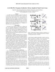
where the angle θ is defined in Figure 4.1. In this case, the sum of equation (4.14) has 

been substituted by the integration on solid angles. In many cases the integration will be 

extended to a restricted domain of solid angles. It is, in particular, the case of the photons 

when they come from a remote source such as the sun. 

The differential variable dH = n2 r cos θ dϖ dA, or its integral on a certain domain 

(at each position of A it must include the solid angle ϖ containing photons), is the 

so-called multilinear Lagrange invariant [10]. It is invariant for any optical system [11]. 

For instance, at the entry aperture of a solar concentrator (think of a simple lens), the 

bundle of rays has a narrow angular dispersion at its entry since all the rays come from 

the sun within a narrow cone. Then, they are collected across the whole entry aperture. 

The invariance for H indicates that it must take the same value at the entry aperture 

and at the receiver, or even at any intermediate surface that the bundle may cross. If 

no ray is turned back, all the rays will be present at the receiver. However, if this 

receiver is smaller than the entry aperture, the angular spread with which the rays illuminate 

the receiver has to be bigger than the angular spread that they have at the entry. 

In this way, H becomes a sort of measure of a bundle of rays, similar to its fourdimensional 

area with two spatial dimensions (in dA) and two angular dimensions (in 

dϖ ). Thus, we may talk of the Hsr of a certain bundle of rays linking the sun with a 

certain receiver. 

Besides Lagrange invariant, this invariant receives other names. In treatises of 

thermal transfer it is called vision or view factor, but Welford and Winston [12] have 

recovered for this invariant the old name given by Poincaré that in our opinion accurately 

reflects its properties. He refers to it as étendue (extension) of a bundle of rays. 

We shall adopt in this chapter this name as a shortened denomination for this multilinear 

Lagrange invariant. 

When the solid angle of illumination consists of the total hemisphere, H = n 2 r πA, 

where A is the area of the surface traversed by the photons. However, in the absence of 

optical elements, the photons from the sun reach the converter located on the Earth within 

dv 

q 

J x 

Figure 4.1 Drawing used to show the flux of a thermodynamic variable across a surface element 

dA 

dA


Table 4.1 Several thermodynamic fluxes for photons with energies between εm and εM distributed 

according to a black body law determined by a temperature T and chemical potential µ. Thelast 

line involves the calculations for a full-energy spectrum (εm = 0andεM =∞). One of the results 

(the one containing T 4 ) constitutes the Stefan–Boltzman law 

˙Ω(T,µ,εm,εM,H)= kT 2H 

h 3 c 2 

� εM 

εm 

˙N(T,µ,εm,εM,H)= 2H 

h3c2 � εM 

εm 

˙E(T,µ,εm,εM,H)= 2H 

h3c2 � εM 

εm 

ln(1 − e (µ−ε)/kT )ε 2 dε = 

ε 2 dε 

− 1 = 

e (ε−µ)/kT 

ε 3 dε 

− 1 = 

e (ε−µ)/kT 

� εM 

εm 

� εM 

εm 

� εM 

εm 

˙ω(T, µ, ε, H) dε (I-1) 

˙n(T , µ, ε, H ) dε (I-2) 

˙e(T, µ, ε, H) dε (I-3) 

˙S = ˙E − µ ˙N − ˙Ω 

; ˙F 

T 

. = ˙E − T ˙S = µ ˙N + ˙Ω (I-4) 

˙E(T,0, 0, ∞,H)= (H/π)σSBT 4 ; ˙S(T,0, 0, ∞,H)= (4H/3π)σSBT 3 ; 

σSB = 5.67 × 10 −8 Wm −2 K −4 

a narrow cone of rays. In this case, H = πAsin 2 θs, whereθs is the sun’s semi-angle of 

vision (taking into account the sun’s radius and its distance to Earth), which is equal [13] 

to 0.267 ◦ . No index of refraction is used in this case because the photons come from 

the vacuum. 

Fluxes of some thermodynamic variables and some formulas of interest, which can 

be obtained from the above principles, are collected in Table 4.1. 

4.2.6 Thermodynamic Functions of Electrons 

For electrons, the number of particles in a quantum state with energy ε is given by 

the Fermi–Dirac function fFD ={exp[(ε − εF )/kT ] + 1} −1 where the electrochemical 

potential (the chemical potential including the potential energy due to electric fields) of 

the electrons is usually called Fermi level, εF . Unlike photons, electrons are in continuous 

interaction among themselves, so that finding different temperatures for electrons is rather 

difficult. In fact, once a monochromatic light pulse is shined on the semiconductor, the 

electrons or holes thermalise to an internal electron temperature in less than 100 fs. 

Cooling to the network temperature will take approximately 10 to 20 ps [14]. However, 

electrons in semiconductors are found in two bands separated by a large energy gap in 

which electron states cannot be found. The consequence of this is that, in non-equilibrium, 

different electrochemical potentials, εFc and εFv (also called quasi-Fermi levels), can exist 

for the electrons in the conduction band (CB) and the valence band (VB), respectively. 

Sometimes we prefer to refer to the electrochemical potential of the holes (empty states 

at the VB), which is then equal to −εFv. Once the excitation is suppressed, it can even 

take milliseconds before the two quasi-Fermi levels become a single one, as it is in the 

case of silicon. 

(I-5)


4.3 PHOTOVOLTAIC CONVERTERS 

4.3.1 The Balance Equation of a PV Converter 

In 1960, Shockley and Queisser (SQ) published an important paper [2] in which the 

efficiency upper limit of a solar cell was presented. In this article it was pointed out, for 

the first time in solar cells, that the generation due to light absorption has a detailed balance 

counterpart, which is the radiative recombination. This SQ efficiency limit, detailed below, 

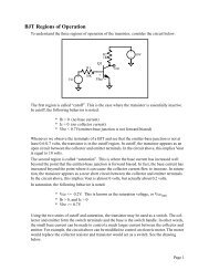
occurs in ideal solar cells that are the archetype of the current solar cells. Such cells 

(Figure 4.2) are made up of a semiconductor with a VB and a CB, more energetic and 

separated from the VB by the band gap, εg. Each band is able to develop separate quasi- 

Fermi levels, εFc for the CB and εFv for the VB, to describe the carrier concentration 

in the respective bands. In the ideal SQ cell the mobility of the carriers is infinite, and 

since the electron and hole currents are proportional to the quasi-Fermi level gradients, it 

follows that the quasi-Fermi levels are constant. Contact to the CB is made by depositing 

a metal on an n + -doped semiconductor. The carriers going through this contact are mainly 

electrons due to the small hole density. The few holes passing through this contact are 

accounted for as surface recombination, assumed zero in the ideal case. Similarly, contact 

with the VB is made with a metal deposited on a p-doped semiconductor. The metal 

Fermi levels εF + and εF − are levelled, respectively, to the hole and the electron quasi- 

Fermi levels εFv and εFc at each interface. In equilibrium, the two quasi-Fermi levels 

become just one. 

The voltage V appearing between the two electrodes is given by the splitting of 

the quasi-Fermi levels, or, more precisely, by the difference in the quasi-Fermi levels of 

majority carriers at the ohmic contact interfaces. With constant quasi-Fermi levels and 

ideal contacts, the split is simply 

eF+ − 

− 

qV = εFc − εFv 

Conduction band 

e Fc 

e Fv 

Valence band 

p + n + 

ev eF− qV 

I I 

Contacts 

qV 

e g 

e c 

− 

− 

Figure 4.2 Band diagram of a solar cell with its contacts 

(4.18)

PHOTOVOLTAIC CONVERTERS 121 

Photons are absorbed by pumping electrons from the VB to the CB through the process 

known as electron–hole pair generation. However, as required by the detailed balance, 

the opposite mechanism is also produced so that a CB electron can decay to the VB and 

emit a photon, leading to what is called a radiative recombination process, responsible for 

luminescent light emission. In fact, many of such luminescent photons whose energy is 

slightly above the band gap are reabsorbed, leading to new electron–hole pair generations 

and balancing out the recombinations. Only the recombination processes leading to the 

effective emission of a photon out of the semiconductor produce a net recombination. 

Taking into account that the luminescent photons are emitted isotropically, only those 

photons emitted near the cell faces, at distances in the range of or smaller than the inverse 

of the absorption coefficient, and directed towards the cell faces with small angles (those 

reaching the surface with angles higher that the limit angle will be reflected back) have 

chances to actually leave the semiconductor, and thus to contribute to the net radiative 

recombination. The rare device analyses that account for this re-absorption – not yet very 

common as they are rather involved and the radiative recombination is small in silicon 

and in many thin-film cells – are said to include photon recycling [15]. 

In the ideal SQ cell any non-radiative recombination mechanism, which is an 

entropy-producing mechanism, is assumed to be absent. 

The difference between the electrons pumped to the CB by external photon absorption 

and those falling again into the VB and effectively emitting a luminescent photon 

equals the current extracted from the cell. This can be presented in an equation form as 

I/q = ˙Ns − ˙Nr = 

� ∞ 

εg 

(˙ns −˙nr) dε (4.19) 

where εg = εc − εv is the semiconductor band gap and ˙Ns and ˙Nr are the photon fluxes 

entering or leaving the solar cell, respectively, through any surface. When the cell is 

properly contacted, this current is constituted by the electrons that leave the CB through 

the highly doped n-contact. In a similar balance, in the VB, I/q are also the electrons 

that enter the VB through the highly doped p-contact. Note that the sign of the current 

is the opposite to that of the flow of the electrons. 

Using the nomenclature in Table 4.1, the terms in equation (4.19) for unit-area 

cells are ˙Ns = a ˙N(Ts, 0,εg, ∞,πsin 2 θs) for the cell facing the sun directly or ˙Ns = 

a ˙N(Ts, 0,εg, ∞,π)for the cell under full concentration and ˙Nr = ξ ˙N(Ta,qV,εg, ∞,π) 

where a and ξ are the absorptivity and emissivity of the cell. Ts is the sun temperature 

and Ta is the room temperature. Full concentration means using a concentrator without 

losses that is able to provide isotropic illumination; this is the highest illuminating power 

flux from a given source. The conservation of the étendue requires this concentrator to 

have a concentration C fulfilling the equation Cπ sin 2 θs = πn 2 r ,thatis,C = 46050n2 r . 

This concentration is indeed unrealistic, but it does lead to the highest efficiency. Furthermore, 

it can be proven [16] that when the quasi-Fermi level split is uniform in the 

semiconductor bulk, then a = ξ. We shall assume – from now on in this chapter – that 

the solar cell is thick enough and perfectly coated with antireflection layers so as to 

fully absorb any photon with energy above the band gap energy so that a = ξ = 1for 

these photons.


The assumption ˙Nr = ˙N(Ta,qV,εg, ∞,π) states that the temperature associated 

with the emitted photons is the room temperature Ta. This is natural because the cell is 

at this temperature. However, it also states that the chemical potential of the radiation 

emitted, µph, is not zero but 

µph = εFc − εFv = qV (4.20) 

This is so because the radiation is due to the recombination of electron–hole pairs, each 

one with a different electrochemical potential or quasi-Fermi level. A plausibility argument 

for admitting µph = εFc − εFv is to consider that photons and electron–hole pairs are 

produced through the reversible (i.e. not producing entropy) equation electron + hole ↔ 

photon. Equation (4.20) would then result as a consequence of equalling the chemical 

potentials before and after the reaction. Equation (4.20) can be also proven by solving 

the continuity equation for photons within the cell bulk [16, 17]. 

When the exponential of the Bose–Einstein function is much higher than one, the 

recombination term in equation (4.19) for full concentration can be written as 

˙Nr = 2π 

h 3 c 2 

� ∞ 

εg 

ε 2 � � 

ε − qV 

exp dε 

kTa 

= 2πkT 

h 3 c 2 [4(kT )2 + 2εgkT + ε 2 g ]exp 

� � 

qV − εg 

kTa 

(4.21) 

This equation is therefore valid for εg − qV ≫ kTa. Within this approximation, the current–voltage 

characteristic of the solar cell takes its conventional single exponential 

appearance. In fact, this equation, with the appropriate factor sin 2 θs, isaccurateinall 

the ranges of interest of the current–voltage characteristic of ideal cells under unconcentrated 

sunlight. 

The SQ solar cell can reach an efficiency limit given by 

η = {qV [ ˙Ns − ˙Nr(qV )]}max 

σSBT 4 

s 

(4.22) 

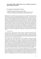
where the maximum is calculated by optimising V . This efficiency limit was first obtained 

by Shockley and Queisser [2] (for unconcentrated light) and is plotted in Figure 4.3 for 

several illumination spectra as a function of the band gap. 

Outside the atmosphere the sun is seen quite accurately as a black body whose 

spectrum corresponds to a temperature of 5758 K [19]. To stress the idealistic approach 

of this chapter, we do not take this value in most of our calculations but rather 6000 K 

for the sun temperature and 300 K for the room temperature. 

It must be pointed out that the limiting efficiency obtained for full concentration 

can be obtained also at lower concentrations if the étendue of the escaping photons is 

made equal to that of the incoming photons [16]. This can be achieved by locating the 

cell in a cavity [20] that limits the angle of the escaping photons.

LIVE GRAPH 

Click here to view 

Efficiency h 

[%] 

45 

40 

35 

30 

25 

20 

15 

10 

40.7% 

5 

1.1 eV 

0 

0.0 0.5 1.0 1.5 2.0 2.5 


a 

d 

b 

c 

Band gap energy E g 

[eV] 

Figure 4.3 SQ efficiency limit for an ideal solar cell versus band gap energy for unconcentrated 

black body illumination, for full concentrated illumination and for illumination under the 

terrestrial sun spectrum: (a) unconcentrated 6000 K black body radiation (1595.9 Wm −2 ); 

(b) full concentrated 6000 K black body radiation (7349.0 × 10 4 Wm −2 ); (c) unconcentrated 

AM1.5-Direct [18] (767.2 Wm −2 ) and (d) AM1.5 Global [18] (962.5 Wm −2 ) 

It is interesting to note that the SQ analysis limit does not make any reference to 

semiconductor pn junctions. William Shockley, who first devised the pn-junction operation 

[21], was also the first in implicitly recognising [2] its secondary role in solar cells. 

In fact, a pn junction is not a fundamental constituent of a solar cell. What seems to be 

fundamental in a solar cell is the existence of two gases of electrons with different quasi- 

Fermi levels (electrochemical potentials) and the existence of selective contacts [22] that 

are traversed by each one of these two gases. The importance of the role of the existence 

of these selective contacts has not been sufficiently recognised. This is achieved today 

with n-andp-doped semiconductor regions, not necessarily forming layers, as in the point 

contact solar cell [23], but in the future it might be achieved otherwise, maybe leading to 

substantial advancements in PV technology. The role of the semiconductor, of which the 

cell is made, is to provide the two gases of electrons that may have different quasi-Fermi 

levels owing to the gap energy separation that makes the recombination difficult. 

So far, for non-concentrated light, the most efficient single-junction solar cell, 

made of GaAs, has achieved an efficiency of 25.1% [24] of AM1.5G spectrum. This is 

only 23% below the highest theoretical efficiency of 32.8% for the GaAs band gap, of 

1.42 eV, for this spectrum [25]. The theoretical maximum almost corresponds to the 

GaAs band gap. However, most cells are manufactured so that the radiation is also 

emitted towards the cell substrate located in the rear face of the cell, and little radiation, 

if any, turns back to the active cell. The consequence of this is that the étendue 

of the emitted radiation, which is π for a single face radiating to the air, is enlarged. 

The étendue is then π + πn 2 r .Thetermπn2 r 

proceeds from the emission of photons 

towards the substrate of the cell, which has a refraction index nr. This reduces the limiting 

efficiency of the GaAs solar cell from 32.8 to 30.7%. Taking this into account, the 

efficiency of this best experimental cell is only 18.2% below the achievable efficiency of 

this cell, only on the basis of radiative recombination. Some substantial increase in efficiency 

might then be achieved by putting a reflector at the rear side of the active layers


of the cells [26] (not behind the substrate!). This would require the use of thin GaAs 

solar cells [27] or the fabrication of Bragg reflectors [28] (a stack of thin semiconductor 

layers of alternating refraction indices) underneath the active layers. Bragg reflectors 

have been investigated for enhancing the absorption of the incoming light in very thin 

cells, but the reduction of the luminescent emission towards the substrate might be an 

additional motivation. 

4.3.2 The Monochromatic Cell 

It is very instructive to consider an ideal cell under monochromatic illumination. When 

speaking of monochromatic illumination, we mean that, in fact, the cell is illuminated 

by photons within a narrow interval of energy �ε around the central energy ε. The 

monochromatic cell must also prevent the luminescent radiation of energy outside the 

range �ε from escaping from the converter. 

For building this device an ideal concentrator [29] can be used that collects the 

rays from the solar disc, with an angular acceptance of just θs, with a filter on the entry 

aperture, letting the aforementioned monochromatic illumination to pass through. This 

concentrator is able to produce isotropic illumination at the receiver. By a reversal of the 

ray directions, the rays issuing from the cell in any direction are to be found also at the 

entry aperture with directions within the cone of semi-angle θs. Those with the proper 

energy will escape and be emitted towards the sun. The rest will be reflected back into 

the cell where they will be recycled. Thus, under ideal conditions no photon will escape 

with energy outside the filter energy and, furthermore, the photons escaping will be sent 

directly back to the sun with the same étendue of the incoming bundle Hsr. 

The current in the monochromatic cell, �I, will then be given by 

�I/q ≡ i(ε,V )�ε/q = (˙ns −˙nr)�ε 

= 2Hsr 

h3c2 ⎡ 

⎢ 

ε 

⎣ 

2�ε ε 

� � − 

ε 

exp − 1 

kTs 

2 ⎤ 

�ε ⎥ 

� � ⎥ 

ε − qV ⎦ 

exp − 1 

kTa 

This equation allows for defining an equivalent cell temperature Tr, 

ε 

= 

kTr 

ε − qV 

� 

⇒ qV = ε 1 − 

kTa 

Ta 

� 

Tr 

so that the power produced by this cell, � ˙W ,is 

� ˙W = 2Hsr 

h3c2 ⎡ 

⎢ 

ε 

⎣ 

3�ε ε 

� � − 

ε 

exp − 1 

kTs 

3 ⎤ 

� 

�ε ⎥ 

� � ⎥ 

ε ⎦ 1 − 

exp − 1 

kTr 

Ta 

� 

Tr 

� 

= (˙es −˙er)�ε 1 − Ta 

� 

Tr 

(4.23) 

(4.24) 

(4.25)


We realise that the work extracted from the monochromatic cell is the same as 

that extracted from a Carnot engine fed with a heat rate from the hot reservoir 

� ˙q = (˙es −˙er)�ε. However, this similarity does not hold under a non-monochromatic 

illumination because, for a given voltage, the cell equivalent temperature would depend 

on the photon energy ε being unable to define a single equivalent temperature for the 

whole spectrum. Note that the equivalent cell temperatures corresponding to short-circuit 

and open-circuit conditions are Ta and Ts, respectively. 

To calculate the efficiency, � ˙W in equation (4.25) must be divided by the appropriate 

denominator. We could divide by the black body incident energy σSBT 4 

s , but this 

would be unfair because the unused energy that is reflected by the entry aperture could 

be deflected with an optical device and used in other solar converters. We can divide by 

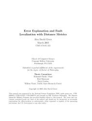
˙es�ε, the rate of power received at the cell, thus obtaining the monochromatic efficiency, 

ηmc, givenby 

ηmc = q(˙ns 

� � 

−˙nr)V � 

� = 1 − 

˙es 

˙er 

�� 

1 − 

˙es 

Ta 

�� 

��max 

(4.26) 

Tr 

� max 

that is represented in Figure 4.4 as a function of the energy ε. 

Alternatively, we could have used the standard definition of efficiency used in 

thermodynamics [30, 31] to compute the efficiency of the monochromatic cell. In this 

context, we put in the denominator the energy really wasted in the conversion process, 

that is, (˙es −˙er)�ε. Actually, the energy ˙er�ε is returned to the sun, perhaps for later 

use (slowing down, for example, the sun’s energy loss process!). This leads to the thermodynamic 

efficiency: 

� 

ηth = 1 − Ta 

� 

(4.27) 

Tr 

This efficiency is the same as the Carnot efficiency obtained by a reversible engine 

operating between an absorber at temperature Tr and the ambient temperature and suggests 

that an ideal solar cell may work reversibly, without entropy generation. Its maximum, 

Efficiency h 

[%] 

100 

95 

90 

85 

80 

75 

70 

65 

LIVE GRAPH 


94.6% 

60 0.0 0.5 1.0 1.5 2.0 2.5 

Energy e 

[eV] 

Figure 4.4 Monochromatic cell efficiency versus photon energy


for � ˙w ≥ 0, is obtained for Tr = Ts, although unfortunately it occurs when � ˙w = 0, that 

is, when negligible (actually, none) work is done by the cell. However, this is a general 

characteristic of reversible engines, which yield the Carnot efficiency only at the expense 

of producing negligible power. 

4.3.3 Thermodynamic Consistence of the Shockley–Queisser 

Photovoltaic Cell 

Electrons and photons are the main particles interacting in a solar cell [8]. However, 

other interactions occur as well. In general, looking at equation (4.13), the generation of 

entropy for each kind of particle (electrons, photons and others) is written as 

σ = � 

i 

� 

1 1 

υ + je∇ 

T T 

µ µ 

− g − jn∇ 

T T +∇· 

� 

− 1 

T jω 

�� 

where the summation extends to the different states of the particle. 

(4.28) 

First we analyse the generation of entropy by electrons, σele. Except for the case 

of ballistic electrons, the pressure – appearing inside jω as shown in equation (4.5) – is 

very quickly equilibrated; it is the same for +v and for −v as a result of the frequent 

elastic collisions. Thus, the term in jω for electrons disappears when the sum is extended 

to all the states in each energy. These collisions also cause the temperature and the free 

energy to become the same for all the directions, at least for a given energy. Furthermore, 

in conventional solar cells, the temperature of the electrons is the same for any energy 

and is equal to the lattice temperature Ta. Also, the electrochemical potential is the same 

for all the electrons within the same band at a given r. 

In a real cell, the energy flow je goes from the high-temperature regions towards 

the low-temperature ones [∇(1/T) ≥ 0] so that the term in (4.28) involving je produces 

positive entropy. The electron flow, jn, opposes the gradient of electrochemical potential, 

thus also producing positive entropy for constant temperature. However, in the ideal 

cell, the lattice temperature, which is also that of the electrons, is constant and the term 

involving ∇(1/T) disappears. Furthermore, in the SQ [2] ideal cell, mobility is infinite 

and, therefore, its conduction and valence band electrochemical potentials or quasi-Fermi 

levels (εFc,εFv) are constant throughout the whole solar cell and their gradients are also 

zero. Therefore, all the gradients in equation (4.28) disappear and the electron contribution 

to entropy generation, σele, isgivenby 

σele = � 

i−ele 

� 1 

υi−ele − 

Ta 

εFc(v) 

gi−ele 

Ta 

� 

(4.29) 

The quasi-Fermi level to be used in this case is εFc or εFv depending on the band to 

which the electronic state i-ele belongs. This is represented by εFc(v). 

Other interactions may occur in the cell involving other particles besides the electrons 

and the photons. We shall assume that in these interactions the bodies involved 

(labelled as others) also have a direction-independent pressure and that they are also at


the lattice temperature. Furthermore, if these particles exist, they are assumed to have 

zero chemical potential (as it is the case, for example, of the phonons). Using these 

assumptions, the contribution to the irreversible entropy generation rate from these other 

particles becomes 

� � 

1 

σothers = � 

i−others 

υi−others 

Ta 

(4.30) 

For the case of the photons, the situation is rather different. As said before, photons do not 

interact with each other and, therefore, they are essentially ballistic. Their thermodynamic 

intensive variables may experience variations with the photon energy and also with their 

direction of propagation. In fact, they come from the sun in a few directions only, and 

only in these directions do they exert a pressure. The direct consequence is that a nonvanishing 

current of grand potential exists for the photons. (It vanishes in gases of photons 

that are confined and in thermal equilibrium with the confining walls. Using this condition 

for photon beams from the sun is not correct.) 

Nph being the number of photons in a mode corresponding to a certain ray moving 

inside the semiconductor, their evolution along a given ray path corresponding to a 

radiation mode is given by [17] 

Nph(ς) = fBE(T , qV )⌊1 − e −ας ⌋+Nph(0)e −ας 

(4.31) 

where ς is the length of the ray, fBE is the Bose–Einstein factor for luminescent photons 

whose chemical potential is the separation between the conduction and the valence band 

electron quasi-Fermi levels – in this case equalling the cell voltage V (times q) –and 

α is the absorption coefficient. Equation (4.31) shows a non-homogeneous profile for 

Nph contributed to by luminescent photons that increase with ς (first term on the righthand 

side) and externally fed photons that decrease when the ray proceeds across the 

semiconductor (second term), and these photons are absorbed. Nph(0) = fBE(Ts, 0) is 

usually taken in solar cells that correspond to illumination by free (i.e. with zero chemical 

potential) radiation at the sun temperature Ts. 

In general, the photons in a mode of energy ε are considered as a macroscopic 

body [9] for which temperature and chemical potential can be defined. However, thermodynamically, 

they can be arbitrarily characterised by a chemical potential µ and a 

temperature T as long as (ε − µ)/T takes the same value. For example, the incident 

solar photons may be considered at the solar temperature Ts with zero chemical potential 

or, alternatively, at room temperature Ta with an energy variable chemical potential 

µs = ε(1 − Ta/Ts). This property has already been used in the study of the monochromatic 

cell. 

Indeed, this arbitrary choice of T and µ does not affect the entropy production. 

This becomes evident if we rewrite equation (4.28) in the case of photons as 

σph = � 

� � � � 

ε − µ ε − µ 

g + jn∇ +∇· − 

T 

T 

1 

T jω 

�� 

(4.32) 

i−ph 

where we have made use of equation (4.15) and of the fact that υ = εg. This equation 

depends explicitly only on (ε − µ)/T . This is less evident in the term in jω/T, but as


discussed in the context of equation (4.15), jω is proportional to T and thus jω/T only 

depends on (ε − µ)/T . Note, however, that jω is affected by the specific choice of T . 

For simplicity, we shall consider the photons at room temperature and we shall 

calculate their chemical potential, µph, from setting the equality 

ε 2 

Nph(ς, ε) = � � 

ε − µph(ς, ε) 

exp 

− 1 

kTa 

(4.33) 

However, we might have chosen to leave µph = 0, and then the effect of the absorption 

of light when passing through the semiconductor could have been described as a cooling 

down of the photons (if Nph actually decreases with ς). 

With the room-temperature luminescent photon description, the production of 

entropy by photons is given by 

σph = � 

� 

υi−ph 

Ta 

i−ph 

− µi−phgi−ph 

Ta 

However, using equations (4.15) and (4.3), 

and 

where 

∇jω = c 

Unr 

σph = � 

− jn,i−ph∇µi−ph 

Ta 

− ∇jω,i−ph 

� 

Ta 

(4.34) 

dΩ c 

∇µ =− fBE∇µ =−jn∇µ (4.35) 

dµ Unr 

i−ph 

� 

− υi−ph 

Ta 

+ µi−phgi−ph 

� 

Ta 

(4.36) 

g = (c/Unr)αfBE(Ta, qV )e −ας − (c/Unr)αfBE(Ts, 0)e −ας ; υ = εg (4.37) 

The total irreversible entropy production is obtained by adding equations (4.29), (4.30) 

and (4.36), taking into account equation (4.37). Now, the terms in energy generation, 

all at the same temperature, must balance out by the first principle of thermodynamics. 

The net absorption of photons corresponds to an electron transfer (positive and negative 

generations) between states gaining an electrochemical potential qV, sothetermsµg/T 

corresponding to electrons and photons subtract each other. No additional generations are 

assumed to take place. Thus the total irreversible entropy generation rate can be written as 

σirr = cα � (µi−ph − qV )[fBE(Ts, 0)e 

Unr 

−ας − fBE(Ta, qV )e−ας ] 

Ta 

i−ph 

(4.38) 

For a given mode the second factor balances out when fBE(Ts, 0) = fBE(Ta, qV ), andso 

does the irreversible entropy generation. In this case, Nph = fBE(Ta, qV ) is constant along 

the ray and µi−ph = qV is constant at all points. The irreversible entropy generation rate is


then zero everywhere. If f(Ts, 0) >f(Ta, qV ), thenNph >f(Ta, qV ) and µi−ph > qV , 

so that both factors are positive and so is the product. If f(Ts, 0)


The second law of thermodynamics, expressed by equations (4.8) and (4.10), integrated 

into the whole volume of the converter can be written, for the stationary case, as 

˙Sirr = 

� 

U 

� 

σirr dU = 

A 

� 

js,i dA = ˙Sr − ˙Ss + ˙Smo − ˙Smi + ˙Sothers 

i 

(4.41) 

The irreversible rate of entropy production is obtained by the elimination of the terms 

with subscript others by multiplying equation (4.41) by Ta, subtracting equation (4.39) 

from the result and taking into account (4.40). In this way we obtain 

Ta ˙Sirr = ( ˙Es − Ta ˙Ss) − ( ˙Er − Ta ˙Sr) + ( ˙Emi − Ta ˙Smi) − ( ˙Emo − Ta ˙Smo) (4.42) 

From equation I-4 (Table 4.1) and considering the annihilation of the grand canonical 

potential flow for electrons, ( ˙Emi − Ta ˙Smi) = εFv ˙Nmi and ( ˙Emo − Ta ˙Smo) = εFc ˙Nmo, so 

that we can write 

Ta ˙Sirr = εFv ˙Nmi − εFc ˙Nmo + ( ˙Es − Ta ˙Ss) − ( ˙Er − Ta ˙Sr) (4.43) 

Taking into account that ˙Nmi = ˙Nmo = I/q and εFc − εFv = qV , equation (4.43) is now 

rewritten as 

Ta ˙Sirr =−˙W + ( ˙Es − Ta ˙Ss) − ( ˙Er − Ta ˙Sr) (4.44) 

Here, this equation has been derived from the local model. However, it can also be 

obtained with more generality from a classical formulation of the second law of thermodynamics 

[32]. It is valid for ideal as well as for non-ideal devices. The values 

of the thermodynamic variables to be used in equation (4.44) are given in Table 4.1. 

Power – which in other cases will be that of the converter under study – corresponds 

in this case to the power of an SQ ideal solar cell and is given by the product of 

equations (4.18) and (4.19). 

We have already discussed the basic ambiguity for the thermodynamic description 

of any radiation concerning the choice of the temperature and the chemical potential. A 

useful corollary is derived from this fact [32]. If the power rate produced by a radiation 

converter depends on the radiation only through its rate of incident energy or number of 

photons, then any radiation received or emitted by the converter can be changed into a 

luminescent radiation at room temperature, Ta, and with chemical potential, µx, without 

affecting the rate of power and of irreversible entropy produced. The chemical potential 

µx of this equivalent luminescent radiation is linked to the thermodynamic parameters of 

the original radiation, Trad and µrad, through the equation 

ε − µrad 

kT rad 

= ε − µx 

kTa 

� 

⇒ µx = ε 1 − Ta 

� 

Trad 

Ta 

+ µrad 

Trad 

(4.45) 

Note that, in general, µx is a function of the photon energy, ε, asitmayalsobeTrad 

and µrad.

THE TECHNICAL EFFICIENCY LIMIT FOR SOLAR CONVERTERS 131 

The proof of the theorem is rather simple and is brought in here because it uses 

relationships of instrumental value. It is straightforward to see that 

˙nx =˙nrad; ˙ex = ε ˙nx =˙erad; ˙ωx/Ta =˙ωrad/Trad; ˙erad − T ˙srad = µx ˙nx +˙ωx 

(4.46) 

where, again, the suffix rad labels the thermodynamic variables of the original radiation. 

The equality of the energy and the number of photons of the original and equivalent 

radiation proves that the power production is unchanged. Furthermore, the last relationship 

can be introduced in equation (4.44) to prove that the calculation of the entropy production 

rate also remains unchanged. 

Taking all this into account, the application of equation (4.44) to the SQ solar cell 

is rather simple. Using the SQ cell model for the power and using the room-temperature 

equivalent radiation (of chemical potential µs) of the solar radiation, we obtain 

Ta ˙Sirr 

� ∞ 

=− 

εg 

� ∞ 

= 

− 

εg 

� ∞ 

εg 

qV [˙n(Ta,µs) −˙n(Ta, qV )]dε + 

[qV ˙n(Ta, qV ) +˙ω(Ta, qV )]dε 

[ ˙ω(Ta,µs) −˙ω(Ta, qV )]dε + 

� ∞ 

εg 

� ∞ 

εg 

[µs ˙n(Ta,µs) +˙ω(Ta,µs)]dε 

[(µs − qV )˙n(Ta,µs)]dε (4.47) 

The integrand is zero for qV = µs, but as µs varies with ε it is not zero simultaneously for 

all ε. To prove that it is positive, we differentiate with respect to qV. Usingd˙ω/dµ =−˙n, 

d(Ta ˙Sirr) 

dqV =− 

� ∞ 

εg 

[˙n(Ta,µs) −˙n(Ta, qV )] = I/q (4.48) 

Thus, for each energy, the minimum of the integrand also appears for qV = µs(ε). Since 

this minimum is zero, the integrand is non-negative for any ε and so is the integral, proving 

also the thermodynamic consistence of this cell from the integral perspective. Furthermore, 

the minimum of the entropy, which for the non-monochromatic cell is not zero, occurs 

for open-circuit conditions. However, the ideal monochromatic cell reaches zero entropy 

production, and therefore reversible operation, under open-circuit conditions, and this is 

why this cell may reach the Carnot efficiency, as discussed in a preceding section. 

4.4 THE TECHNICAL EFFICIENCY LIMIT FOR SOLAR 

CONVERTERS 

We have seen that with the technical definition of efficiency – in whose denominator the 

radiation returned to the sun is not considered – the Carnot efficiency cannot be reached 

with a PV converter. What then is the technical efficiency upper limit for solar converters? 

We can consider that this limit would be achieved if we could build a converter 

producing zero entropy [33]. In this case, the power that this converter can produce,


˙Wlim, can be obtained from equation (4.44) by setting the irreversible entropy-generation 

term to zero. Substituting the terms involving emitted radiation by their room-temperature 

luminescent equivalent, equation (4.44) becomes 

� ∞ 

˙Wlim = 

εg 

{[˙es − Ta ˙ss] − [µx(ε)˙nx +˙ωx]} dε = 

� ∞ 

εg 

˙wlim(ε, µx) dε (4.49) 

The integrand should now be maximised [32] with respect to µx. For this, we calculate 

the derivative 

d ˙wlim 

dµx 

d ˙ωx 

=−˙nx − 

dµx 

d˙nx 

− µx 

dµx 

d˙nx 

=−µx 

dµx 

(4.50) 

where we have used that the derivative of the grand potential with respect to the chemical 

potential is the number of particles with a change of sign. This equation shows that the 

maximum is achieved if µx = 0foranyε, or, in other words, if the radiation emitted is 

a room-temperature thermal radiation. This is the radiation emitted by all the bodies in 

thermal equilibrium with the ambient. However, the same result will be also achieved if 

the emitted radiation is any radiation whose room-temperature luminescent equivalent is 

a room-temperature thermal radiation. 

Now, we can determine this efficiency, according to Landsberg [33], as 

� �� 

Hsr 

σT 

π 

η = 

4 

� � 

4 3 

s − σTaTs − σT 

3 4 4 

a − 

3 σT4 

�� 

a 

(Hsr/π)σ T 4 

s 

= 1 − 4 

� � 

Ta 

+ 

3 

1 

� �4 Ta 

3 

Ts 

Ts 

(4.51) 

which for Ts = 6000 K and T = 300 K gives 93.33% instead of 95% of the 

Carnot efficiency. 

No ideal device is known that is able to reach this efficiency. Ideal solar thermal 

converters, not considered in this chapter, have a limiting efficiency of 85.4% [34, 35] 

and therefore do not reach this limit. Other high-efficiency ideal devices considered in 

this chapter do not reach it either. We do not know whether the Landsberg efficiency 

is out of reach. At least it is certainly an upper limit of the technical efficiency of any 

solar converter. 

4.5 VERY HIGH EFFICIENCY CONCEPTS 

4.5.1 Multijunction Solar Cells 

A conceptually straightforward way of overcoming the fundamental limitation of the SQ 

cell, already pointed out by SQ, is the use of several solar cells of different band gaps 

to convert photons of different energies. A simple configuration to achieve it is by just 

stacking the cells so that the upper cell has the highest band gap and lets the photons 

pass through towards the inner cells (Figure 4.5). The last cell in the stack is the one 

with the narrowest band gap. Between cells we put low-energy pass filters so that the

Light 

VERY HIGH EFFICIENCY CONCEPTS 133 

Reflectors 

Cell 1 Cell n Cell N 

Figure 4.5 Stack of solar cells ordered from left to right in decreasing band gap 

(Eg1 >Eg2 >Eg3). (Reprinted from Solar Energy Materials and Solar Cells V. 43, N. 2, Martí A. 

and Araújo G. L, Limiting Efficiencies for Photovoltaic Energy Conversion in Multigap Systems, 

203–222, © 1996 with permission from Elsevier Science) 

reflection threshold of each filter is the band gap of the cell situated above. This prevents 

the luminescent photons from being emitted for energies different to those with which the 

photons from the sun are received in each cell. In this configuration, every cell has its own 

load circuit, and therefore, is biased at a different voltage. It has been shown [31] that a 

configuration without back reflectors leads to a lower efficiency if the number of cells is 

finite. For the case of a stack with an infinite number of cells, the limiting efficiency is 

found to be independent of whether reflectors are placed or not. 

For example, for the case of a stack with two cells, the power generated is 

W = qVl⌊ ˙N(Ts, 0,εgl,εgh,Hs) − ˙N(Ta,qVl,εgl,εgh,Hr)⌋ 

+ qVh[ ˙N(Ts, 0,εgh, ∞,Hs) − ˙N(Ta,qVh,εgh, ∞,Hr)] (4.52) 

where the suffixes l and h (low and high) refer to the band gap and the voltage of the 

two cells involved. The maximum power is obtained by optimising this function with 

respect to the variables Vl, Vh, εgl and εgh. We present in Figure 4.6 the efficiency of 

High band gap 

[eV] 

Low band gap 

[eV] 

Figure 4.6 Efficiency of a tandem of two ideal cells under AM1.5D illumination as a function of 

the two cells’ band gap εl and εh


two ideal cells as a function of the two cells’ band gaps, which is optimised only with 

respect to Vl and Vh. The generation term is in this case not the one in equation (4.52) 

but the one corresponding to a standard spectrum AM1.5D [18]. Power is converted into 

efficiency by dividing by 767.2 Wm −2 , which is the power flux carried by the photons in 

this spectrum. In the figure, we can observe that the efficiency maximum is very broad, 

allowing for a wide combination of materials. 

A lot of experimental work has been done on this subject. To our knowledge, the 

highest efficiency so far achieved, 34% (AM1.5 Global), has been obtained by Spectrolab 

[24, 36], in 2001, using a monolithic (made on the same chip) two-terminal tandem 

InGaP/GaAs stuck on a Ge cell and operating at a concentration factor of 210, that is, at 

21 Wcm −2 . 

The maximum efficiency is obtained with an infinite number of solar cells, each 

one biased at its own voltage V(ε) and illuminated with monochromatic radiation. The 

efficiency of this cell is given by 

η = 

� ∞ 

0 

ηmc(ε)˙es dε 

� ∞ 

0 

˙es dε 

= 1 

σSBT 4 

s 

� ∞ 

0 

ηmc(ε)˙es dε = 1 

σSBT 4 

s 

� ∞ 

0 

i(ε,V )V |max dε (4.53) 

where ηmc(ε) is the monochromatic cell efficiency given by equation (4.26) and i(ε,V ) 

was defined in equation (4.23). For Ts = 6000 K and Ta = 300 K, the sun and ambient 

temperature, respectively, this efficiency is [34] 86.8%. This is the highest efficiency limit 

of known ideal converter. 

Tandem cells emit room-temperature luminescent radiation. This radiation presents, 

however, a variable chemical potential µ(ε) = qV (ε) and therefore it is not a radiation 

with zero chemical potential (free radiation). In addition, the entropy produced by this 

array is positive since the entropy produced by each one of the monochromatic cells 

forming the stack is positive. None of the conditions for reaching the Landsberg efficiency 

(zero entropy generation rate and emission of free radiation at room temperature) is then 

fulfilled and, therefore, tandem cells do not reach this upper bound. 

It is highly desirable to obtain monolithic stacks of solar cells, that is, on the same 

chip. In this case, the series connection of all the cells in the stack is the most compact 

solution. Chapter 9 will deal with this case extensively. If the cells are series-connected, 

a limitation appears that the same current must go through all the cells. For the case of 

two cells studied above, this limitation is expressed by the equation 

I = q⌊ ˙N(Ts, 0,εgl ,εgh,Hs) − ˙N(Ta,qVl,εgl,εgh,Hr)⌋ 

= q[ ˙N(Ts, 0,εgh, ∞,Hs) − ˙N(Ta,qVh,εgh, ∞,Hr)] (4.54) 

This equation establishes a link between Vl and Vh (for each couple εl, εh), which reduces 

the value of the maximum achievable efficiency. The total voltage obtained from the stack 

is V = Vl + Vh. 

Our interest now is to determine the top efficiency achievable in this case when 

the number of cells is increased to infinity. Surprisingly enough, it is found [37, 38] that


the solution is also given by equation (4.53) and therefore, the limiting efficiency of a set 

of cells that is series-connected is also 86.8%. 

4.5.2 Thermophotovoltaic Converters 

Thermophotovoltaic (TPV) converters are devices in which a solar cell converts the radiation 

emitted by a heated body into electricity. This emitter may be heated, for example, by 

the ignition of a fuel. However, in our context, we are more interested in solar TPV converters 

in which the sun is the source of energy that heats an absorber at temperature Tr, 

which then emits radiation towards the PV converter. Figure 4.7 draws the ideal converter 

for this situation. 

An interesting feature of the TPV converter is that the radiation emitted by the 

solar cells is sent back to the absorber assisting in keeping it hot. To make the cell area 

different from the radiator area (so far cells in this chapter have all been considered to be 

of area unity), the absorber in Figure 4.7 radiates into a reflecting cavity containing the 

cell. The reflective surfaces in the cavity and the mirrors in the concentrator are assumed 

to be free of light absorption. 

In the ideal case [39], the radiator emits two bundles of rays, one of étendue Hrc 

(emitted by the right side of the absorber in the Figure 4.7a), which is sent to the cell after 

reflections in the cavity walls, with energy E ′ r without losses, and another (unavoidable) 

one Hrs, with energy Er, which is sent back to the sun (by the left face of the absorber) 

after suffering reflections in the left-side concentrator. Ideally, the radiator illuminates no 

other absorbing element or dark part of the sky: all the light emitted by the radiator’s 

left side is sent back to the sun by the concentrator. Rays emitted by the radiator into the 

cavity may return to the radiator again without touching the cell, but since no energy is 

transferred, such rays are not taken into account. 

Absorber 

Cell & filter 

(PV converter) 

A i Inlet A r A c 

Concentrator 

Cavity 

· 

Es · 

Er PV 

converter 

Absorber at T r 

· · 

Er ′ Ec · 

Qs Environment at T a 

(a) (b) 

Figure 4.7 (a) Schematic of an ideal TPV converter with the elements inserted in loss-free 

reflecting cavities and (b) illustration of the thermodynamic fluxes involved. In the 

monochromatic case, ˙Es ≡ ˙E(Ts, 0, 0, ∞,Hrs), ˙Er ≡ ˙E(Tr, 0, 0, ∞,Hrs), ˙E ′ r ≡˙e(ε, Tr, 0,Hrc)�ε, 

˙Ec ≡˙e(ε, Ta,qV,Hrc)�ε 

W ·


On the other hand, the radiator is illuminated by a bundle of rays, coming from 

the sun, of étendue Hsr = Hrs and by the radiation emitted by the cell itself, of étendue 

Hcr = Hrc. Also, the cell may emit some radiation into the cavity, which returns to the 

cell again. This radiation is therefore not accounted for as an energy loss in the cell. 

In addition, we shall assume that the cell is coated with an ideal filter that allows only 

photons with energy ε and within a bandwidth �ε to pass through, while the others are 

totally reflected. In this situation the energy balance in the radiator becomes 

˙E(Ts, 0, 0, ∞,Hrs) +˙e(ε, Ta, qV ,Hrc)�ε =˙e(ε, Tr, 0,Hrc)�ε + ˙E(Tr, 0, 0, ∞,Hrs) 

(4.55) 

where the first equation member is the net rate of energy received by the radiator and the 

second member is the energy emitted. 

Using ˙e(ε, Tr, 0,Hrc)�ε −˙e(ε, Ta, qV ,Hrc)�ε = ε�i/q = ε� ˙w/(qV ),where�i 

is the current extracted from the monochromatic cell and � ˙w is the electric power delivered, 

it is obtained that 

ε� ˙w 

qV 

HrsσSB 

= (T 

π 

4 4 

s − Tr ) ⇔ ε2�i Hrsε 

= 

qH rc�ε Hrc�ε 

σSB 4 

(Ts π 

4 

− Tr ) (4.56) 

This equation can be used to determine the operation temperature of the radiator, Tr, as 

a function of the voltage V , the sun temperature Ts, the energy ε and the dimensionless 

parameter Hrc�ε/Hrsε. Notice that the left-hand side of equation (4.56) is independent 

of the cell étendue and of the filter bandwidth (notice that �i ∝ Hrc�ε). 

Dividing by HrsσSBT 4 

s 

of the TPV converter as 

η = 

� 

1 − 

/π, the solar input power, allows expressing the efficiency 

4 Tr T 4 

�� 

qV 

= 1 − 

s ε 

4 Tr T 4 

�� 

s 

1 − Ta 

Tc 

� 

(4.57) 

where Tc is the equivalent cell temperature as defined by equation (4.24). As presented 

in Figure 4.8, this efficiency is a monotonically increasing function of Hrc�ε/Hrsε. For 

(Hrc�ε/Hrsε) →∞, �i → 0andTr → Tc. In this case an optimal efficiency [40] for 

Ts = 6000 K and Ta = 300 K is found to be 85.4% and is obtained for a temperature 

Tc = Tr = 2544 K. This is exactly the same as the optimum temperature of an ideal solar 

thermal converter feeding a Carnot engine. In reality, the ideal monochromatic solar cell is 

a way of constructing the Carnot engine. This efficiency is below the Landsberg efficiency 

(93.33%) and slightly below the one of an infinite stack of solar cells (86.8%). 

It is worth noting that the condition (Hrc�ε/Hrsε) →∞requires that Hrc ≫ Hrs, 

and for this condition to be achieved, the cell area must be very large compared to the 

radiator area. This compensates the narrow energy range in which the cell absorbs. This 

is why a mirrored cavity must be used in this case. 

4.5.3 Thermophotonic Converters 

A recent concept for solar conversion has been proposed [3] with the name of thermophotonic 

(TPH) converter. In this concept, a solar cell converts the luminescent radiation

Efficiency h 

[%] 

100 

90 

80 

70 

60 

50 

40 

30 

20 

10 

85.4% 

2544 K 


1 10 

100 

(∆eHrc )/(eHrs ) 

2000 

0 

LIVE GRAPH 


Figure 4.8 TPV ideal converter efficiency versus Hrc�ε/Hrsε. The energy ε and the cell voltage 

V are optimised 

Hot cell 

(LED) 

Cold cell 

A i inlet A r A c 

Concentrator 

(a) 

Cavity 

· 

Es · 

Er Hot cell (LED) T r 

Cold 

cell 

· · 

Er′ Ec Environment at T a 

Figure 4.9 Diagram of the TPH converter with cavity. In (b), the energy fluxes are given 

by ˙Es ≡ E(Ts, 0, 0, ∞,Hrs), ˙Er ≡ E(Tr,qVr, 0, ∞,Hrs), ˙Qr = ˙Es − ˙Er, ˙E ′ r ≡ E(Tr,qVr, 0, ∞,Hrc), 

˙E ′ c ≡ E(Ta,qVc,εg, ∞,Hrc) 

emitted by a heated light emitting diode (LED) into electricity. A diagram of this device 

is found in Figure 4.9. As in the TPV device, the LED can be heated with a fuel, but in 

our context it is heated as well with radiation absorbed from the sun. To emit luminescent 

radiation, the LED absorbs electric power, ˙Wr, in addition to the power delivered from 

the photons that illuminate the absorber. This power is to be subtracted from the electric 

power converted by the solar cell ˙Wc. 

· 

Qc (b) 

6000 

5500 

5000 

4500 

4000 

3500 

3000 

2500 

· 

Wc Temperature of the radiator Tr [K] 

· 

Wr W ·


As a mater of fact, this converter is a generalisation of the TPV converter. If the 

LED is in short circuit, the TPH converter is exactly the same as the TPV converter. The 

application of a voltage to the LED changes the converter properties. 

Ideal LEDs are like solar cells. Thus, to describe the ideal TPH converter, we shall 

refer to the LED as the hot cell, as opposed to the electric power generator, which is the 

cold cell. When they are considered as ideal devices, the current–voltage characteristics 

of both, the LED and the solar cell, are the same. This causes the current passing by the 

cold cell to be faithfully replicated (with the sign changed) by the hot cell, owing to the 

reciprocal illumination of both devices, as expressed by the two following equations: 

Ic/q = ˙N(Tr,qVr,εg, ∞,Hrc) − ˙N(Ta,qVc,εg, ∞,Hrc) (4.58) 

Ir/q = ˙N(Ta,qVc,εg, ∞,Hrc) − ˙N(Tr,qVr,εg, ∞,Hrc) (4.59) 

We shall use the subindex c for the cold solar cell current and voltage and r for the hot 

solar cell. The power generated by each cell is ˙Wc = IcVc and ˙Wr = IrVr. In a normal 

operation, Ir is negative and the power generated by the hot cell is negative. 

The application of the first law of thermodynamics to the cold and the hot cell, 

respectively, leads to 

˙E(Tr,qVr,εg, ∞,Hrc) = ˙E(Tc,qVc,εg, ∞,Hrc) + ˙Wc + ˙Qc 

˙Qr + ˙E(Tc,qVc,εg, ∞,Hrc) = ˙E(Tr,qVr,εg, ∞,Hrc) + ˙Wr 

where ˙Qc is the heat rate delivered by the cold cell in the heat sink, while 

˙Qr = ˙E(Ts, 0, 0, ∞,Hrs) − ˙E(Tr, 0, 0, ∞,Hrs) = HsrσSB 

(T 

π 

4 

s 

(4.60) 

(4.61) 

4 

− Tr ) (4.62) 

is the heat injected by the sun into the hot cell. The sum of equations (4.60) and (4.61) 

leads to 

˙Qr − ˙Qc = ˙Wr + ˙Wc = Ir(Vr − Vc) = Ic(Vc − Vr) = ˙W (4.63) 

where ˙W is the algebraic sum of the powers produced by both cells (usually the hot cell 

will be absorbing, not producing, power). 

In the case of monochromatic cell and LED operation, a proper filter of bandwidth 

�ε and centred at the energy ε is to be located somewhere in the optical system to allow 

for an interchange of photons only within the filter bandwidth. The preceding equations 

can be easily particularised in this case. An interesting relationship holding in this case, 

˙e�ε = ε ˙n�ε ≡ ˙E, allows for a simple expression of the heat rate in both cells, 

˙Qr = (Vr − ε/q)Ir 

˙Qc = (ε/q − Vc)Ic 

(4.64) 

(4.65)


and this allows for writing the efficiency, using the equations (4.63) to (4.65) as 

η = 

˙Qr 

HsrσSBT 4 

s /π 

˙W 

˙Qr 

= 

� 

1 − 

4 Tr T 4 

� 

s 

� 

1 − ˙Qc 

� � 

= 1 − 

˙Qr 

T 4 

r 

T 4 

s 

�� 

qVc/ε − qVr/ε 

1 − qVr/ε 

(4.66) 

As said before, the TPH converter has an extra degree of freedom in the design, as 

compared to the TPV. It is the hot cell voltage Vr. The hot cell temperature in the 

monochromatic case depends on the same parameter Hrc�ε/Hrsε as in the TPV case. 

When this parameter tends to infinity, the cold cell tends to be in open circuit, Vcoc, 

given by 

(ε − qVcoc) 

= 

kTa 

(ε − qVr) 

kTr 

� 

⇒ qVcoc = ε 

1 − Ta 

Tr 

� 

Ta 

+ qVr 

Tr 

(4.67) 

Using this equation in equation (4.66), we obtain the same limit equation for the efficiency 

as the one for the TPV converter (equation 4.57): 

η = 

� 

1 − 

4 Tr T 4 

�� 

s 

1 − Ta 

Tr 

� 

(4.68) 

An interesting feature of this formula is that it holds for any value of Vr. Thus the TPH 

converter has the same upper limit as the TPV one. Furthermore, Tr is the same as in 

the TPV. 

To our knowledge, this novel concept has not yet been fully explored. However, 

we present in Figure 4.10 the efficiency versus the cold cell voltage Vc (usually, in other 

contexts, we call efficiency to the maximum of this curve) for Vr in forward bias, zero bias 

(TPV mode) and reverse bias. In Figure 4.11, we present the hot cell temperature. We can 

Efficiency h 

[%] 

LIVE GRAPH 


90 

80 

70 

60 

50 

40 

30 

20 

10 

0 

−0.5 0.0 

LED bias +0.5 V, e = 1.376 eV 

LED bias +0 V, e = 1.353 eV 

LED bias −0.5 V, e = 1.464 eV 

63.5% 

0.5 

Cell voltage V 

[V] 

82.2% 

75.9% 

1.0 1.5 

Figure 4.10 TPH efficiency versus Vc for three values of Vr for Hrc�ε/Hrsε = 10/π. The energy 

ε has been optimised


Radiator temperature Tr [K] 

LIVE GRAPH 


6000 

5000 

4000 

3000 

2000 

1000 

4364 K 

3551 K 

2574 K 

LED bias +0.5 V, e = 1.376 eV 

LED bias +0 V, e = 1.353 eV 

LED bias −0.5 V, e = 1.464 eV 

0 

−0.5 0.0 0.5 

Cell voltage V 

[V] 

1.0 1.5 

Figure 4.11 Hot cell temperature as a function of the cold cell voltage for several biasing voltages 

of the hot cell (LED) and for the energy that leads to maximum efficiency (Hrc�ε/Hrsε = 10/π). 

The energy ε has been optimised 

see that higher efficiencies at lower temperatures can be obtained using the TPH concept 

under direct bias. This is not in contradiction to the fact that the limiting efficiency and 

the temperature for it is the same in both cases. 

4.5.4 Higher-than-one Quantum Efficiency Solar Cells 

One of the drawbacks that limit the efficiency of single-junction solar cells is the energy 

wasted from each photon that is absorbed because it is not converted into electrical power. 

Werner, Kolodinski, Brendel and Queisser [41, 42] have proposed a cell in which each 

photon may generate more than one electron–hole pair, thus leading to higher-than-one 

quantum efficiency solar cells. Without discussing which physical mechanisms may allow 

for this behaviour, let us examine its implications. Admitting that every photon may create 

m(ε) electron–hole pairs, the current extracted from the device would be given by 

I/q = 

� ∞ 

εg 

[m(ε)˙ns − m(ε)˙nr(T , µ)]dε (4.69) 

In this equation, εg is the energy threshold for photon absorption and the factor m in the 

generation term is our initial assumption. The same term must appear in the recombination 

term to reach the detailed balance: if the sun temperature is brought to the ambient 

temperature, the current will be zero when µ = 0, only if the factor m also appears in the 

recombination term. For the moment we are saying nothing about the chemical potential 

µ of the photons emitted. 

The power delivered, ˙W ,isgivenby 

˙W = 

� ∞ 

εg 

qV [m˙ns − m˙nr(T , µ)]dε (4.70)


Let us consider a monochromatic cell and calculate the irreversible entropy generation 

rate ˙Sirr in the whole device. With the aid of the general equation (4.44) and equation I-4 

in Table 4.1, it is given by 

Ta ˙Sirr/�ε = (µx ˙nx +˙ωx) − (µ ˙nr +˙ωr) − qV (m ˙nx − m˙nr) (4.71) 

where the source of photons has been substituted by its equivalent room-temperature luminescent 

radiation characterised by the chemical potential µx and the ambient temperature 

Ta. The open-circuit conditions are achieved when µOC = µx. For this value the entropy 

rate is zero since then ˙nx =˙nr and ˙ωx =˙ωr. 

Let us calculate the derivative of the irreversible entropy generation rate 

(equation 4.71) with respect to µ and particularise it for the open-circuit value of µ. 

Considering what follows V as only an unknown function of µ and independent of the 

way of obtaining the excitation (which is the case for infinite mobility) and using the 

fundamental relationship ∂ ˙ωr/∂µ =−˙nr, the result is 

� 

d(Ta ˙Sirr/�ε) 

� 

� � 

d˙nr 

= (qmVOC − µOC) 

(4.72) 

dµ 

dµ 

µOC 

This derivative is only zero if qmVOC = µOC. SinceµOC = µx can take any value by 

changing the source adequately, we obtain the result qmV = µ. Any other value would 

produce a negative rate of entropy generation in the vicinity of the open circuit, against 

the second law of thermodynamics. This is a demonstration, based on the second law of 

thermodynamics, of the relationship between the chemical potential of the photons and 

the voltage (or electron and hole quasi-Fermi level split). 

If we could choose m freely, the maximum power is achieved if we can maximise 

the integrand of equation (4.70) for each value of the energy [43, 44]. Once this 

is done, the reduction in εg so that it tends towards zero increases the power output. 

For the limit of εg → 0, the maximum efficiency is the same as in equation (4.53), 

where a stack of an infinite number of cells was studied. Here qV m(ε) is the variable 

that plays the same role as qV (ε) earlier, although here V is the same for all 

the terms. In consequence, the upper efficiency is the same as for the tandem cell 

stack, 86.8%. 

The higher-than-one quantum efficiency behaviour has been actually found [45, 46], 

although very close to one, for visible photons of high-energy and UV photons. The effect 

is attributed to impact ionisation, a mechanism in which the electron or the hole created 

by the high-energy photon, instead of thermalising by scattering with phonons, by means 

of impact processes transfers its high energy to a valence-band electron that gets pumped 

into the conduction band. This mechanism has a detailed balance counterpart that is the 

Auger recombination, in which the energy recovered in the recombination is transferred to 

an electron or a hole, which thus acquires a high kinetic energy. 

4.5.5 Hot Electron Solar Cells 

Wurfel [47] has studied the impact ionisation cells from another perspective and has shown 

that they become identical to the hot carrier solar cells proposed by Ross and Nozik [48] 

µOC


pointing out also in this respect the necessity of providing the cell with special contacts 

as will be explained below. 

In the hot carrier solar cell, the electron gas (semiconductor properties exhibiting 

a band gap does not seem to be essential for its operation) is in equilibrium at the lattice 

temperature Ta despite the absence of phonon interaction. This equilibrium is reached 

through other interactions as, for example, the interaction with thermal photons. Out of 

the equilibrium, electrons are thermalised by elastic scattering between them that allows 

a set of energy-dependent chemical potentials, one for the electrons of each energy. 

Furthermore, transference of energy between electrons exists through mechanisms that 

include impact ionisation and Auger recombination (this terminology is used in the context 

of semiconductors, which, as mentioned, we think is not necessary for this cell) according 

to reactions like e1 − + e2 − ↔ e3 − + e4 − . Actually in this equation transference of energy 

between electrons is produced by couples so that ˆε1 +ˆε2 =ˆε3 +ˆε4 where ˆε is electron 

(not photon) energy. However, the equilibrium of the reaction also establishes that the 

electrochemical potentials of the electrons (that we still call εF ) are related by εF (ˆε1) + 

εF (ˆε2) = εF (ˆε3) + εF (ˆε4). Therefore, the electrochemical potential of the electrons is a 

linear function of the energy in the form 

εF (ˆε) = β ˆε + εF 0 

where the Fermi energy reference εF 0 becomes the same for both electrons and holes. 

Since the Fermi function for electrons is written as 

1 

1 

� � = � � 

ˆε − β ˆε − εF 0 

ˆε − εF 0/(1 − β) 

exp 

+ 1 exp 

+ 1 

kTa 

kTa/(1 − β) 

(4.73) 

(4.74) 

the electron distribution can be regarded equivalently as a distribution at the lattice temperature 

Ta but characterised by a varying electrochemical potential given by equation (4.73) 

or as a hot carrier distribution with a constant electrochemical potential given by µhc = 

εF 0/(1 − β) and a hot carrier temperature Thc = Ta/(1 − β). 

If the interaction with phonons is introduced, through the reaction e1 − + phonon ↔ 

e2 − ,wheree1(2) − represents an electron with energy ˆε1(2), the fact that the phonon chemical 

potential is zero leads to εF (ˆε1) = εF (ˆε2). However, ˆε1 �= ˆε2 but ˆε2 =ˆε1 + ε, where 

ε is the phonon energy and, therefore, εF (ˆε1) = εF (ˆε2) is only fulfilled if β = 0and 

consequently all the electrons have the same electrochemical potential εF 0 and are at the 

lattice temperature. Phonon interaction is not considered to occur in what follows. 

If the interaction with photons is considered now, e1 − + photon ↔ e2 − , the equilibrium 

of the reaction is represented by εF (ˆε1) + µph = εF (ˆε2) where µph is the photon 

chemical potential. Taking into account equation (4.73), it is obtained that µph = 

β(ˆε1 −ˆε2) = βε where ε is the energy of the photon involved. The result is that we have 

an energy-dependent photon chemical potential µph. The Bose function that describes the 

occupation probability of the photon energy level ε becomes 

1 

� � = 

ε − βε 

exp − 1 

kTa 

� 

exp 

1 

ε 

kTa/(1 − β) 

� 

− 1 

(4.75)


which can be seen as free radiation (zero chemical potential) at the hot carrier 

temperature. 

Würfel also points out that, provided we can find a material in which a weak 

phonon coupling is produced in order to manufacture a solar cell, we still should be 

careful with the contacts because they do not allow for the maintenance of hot carriers 

inside the absorbing material. These special contacts must be able to cool the electrons 

from the hot temperature Thc to the contact temperature Ta reversibly by changing their 

electrochemical potential from εF 0 to the electron electrochemical potential at the contacts 

(Fermi level at the metals) εF + and εF −. In Wurfel’s Reference [47], these special contacts 

are devised as selective membranes (Figure 4.12) that only allow electrons with energy 

centred around εe (left contact) and εh (right contact) to pass through. The reversible 

change in temperature and electrochemical potential of the electrons at the membranes is 

obtained by setting 

ˆεe − µhc 

kThc 

ˆεh − µhc 

kThc 

= ˆεe − εF − 

kT a 

= ˆεh − εF + 

kTa 

� 

⇔ εF − =ˆεe 1 − Ta 

� 

Thc 

� 

⇔ εF + =ˆεh 1 − Ta 

� 

Thc 

Ta 

+ µhc 

Thc 

Ta 

+ µhc 

Thc 

where Thc = Ta/(1 − β). The cell voltage will therefore be given by 

� 

qV = εF − − εF + = (ˆεe −ˆεh) 1 − Ta 

� 

Thc 

(4.76) 

(4.77) 

The current extracted from the cell is determined by the rate at which electron–hole pairs 

of energy ˆεe −ˆεh can be withdrawn from the cell. Since no energy is lost as heat, the 

energy balance equation (first principle) leads to 

I(ˆεe −ˆεh)/q = ˙E(Ts, 0,εg, ∞,Hs) − ˙E(Thc, 0,εg, ∞,Hr) (4.78) 

+ 

∆ 

eV 

Metal Electron Absorber Hole Metal 

membrane 

membrane 

Figure 4.12 Band structure of a hot electron solar cell showing contacting scheme by means 

of selective membranes. (Reprinted from Solar Energy Materials and Solar Cells V. 46, N. 1, 

Würfel P., Solar Energy Conversion with Hot Electrons from Impact Ionisation, 43–52, © 1997 

with permission from Elsevier Science) 

∆


and the power extracted from the cell can be finally computed as 

� 

˙W = IV = [ ˙E(Ts, 0,εg, ∞,Hs) − ˙E(Thc, 0,εg, ∞,Hr)] 1 − Ta 

� 

Thc 

(4.79) 

which is independent of the carrier-extracting energies of the contacts. In other words, 

a large separation of the extracting energies leads to high voltage and low current and 

vice versa. Note that Thc is a parameter for equation (4.79) and for equation (4.77). By 

elimination, we obtain the W(V) and from it the derived IV curve. The cell efficiency is 

obtained from the maximum of W(V) or W(Thc). 

For εg → 0 the limit efficiency becomes 

� 

η = 1 − T 4 hc 

T 4 

� � 

1 − 

s 

Ta 

� 

Thc 

just as in the TPV converters, leading to a limiting efficiency of 85.4%. 

(4.80) 

The monoenergetic membrane for electron and hole transfer to the contacting 

metals might perhaps be an insulator with an impurity band, but the nature of the phononinsulated 

absorber is totally unknown. Ross and Nozik [48, 49] who have developed 

concepts close to those expressed here are investigating the poorer coupling of the electrons 

with the photons in materials with quantum dots with the idea of favouring this 

hot electron type of cell or the impact ionisation one that we have described in the 

preceding section. 

4.5.6 Intermediate Band Solar Cell 

One of the causes of efficiency reduction in single-junction solar cells is the transparency 

of the semiconductor to sub–band gap photons [50]. The inclusion of an intermediate 

band (IB) may greatly increase the efficiency. We show in Figure 4.13 a band diagram 

of the photon absorption and emission in this intermediate band material. Photons are 

absorbed not only by pumping electrons from the VB to the CB as in a traditional solar 

cell (photons with energy hν3) but also by transitions from the VB to the IB (photons 

with energy hν2) and from the IB to the CB (photons with energy hν1). In total, two lowenergy 

photons are used to pump an electron from the valence band to the conduction 

band, passing through the intermediate band. This certainly increases the cell current. 

The three absorption mechanisms detailed above are effective if the IB is a band 

partially filled with electrons. In this way, there are empty states in it to accommodate 

the electrons from the VB and there are electrons to sustain a strong pumping to the CB. 

The detailed balance imposes photon emissions that are opposite to each one of the three 

absorption mechanisms. 

The cell is contacted as shown in Figure 4.14. The electrons are extracted from the 

VB and returned to the CB using two layers of n and p ordinary semiconductors. A high 

voltage is produced as the sum of the two semiconductor junction voltages occurring at 

both sides of the IB material.

Intermediate 

band 

hv 1 

hv 2 



hv 3 

Valence band 

Figure 4.13 The band diagram of an intermediate band solar cell 

In this IB material we admit that there are three quasi-Fermi levels, one for each 

band. The cell voltage is q times the splitting of the CB and VB quasi-Fermi levels. 

In general, there is an energy threshold for each one of the absorption mechanisms 

described earlier. However, the ideal structure is the one in which the upper energy (lintel) 

of a photon that can be absorbed in certain mechanisms – involving, for example, transitions 

from the VB to the IB – is the threshold of the next one – for example, transitions 

from the IB to the CB. More specifically, calling εg the energy interval between the conduction 

and the valence band, εl the interval between the Fermi level in the intermediate 

band and the valence band and εh = εg − εl, and assuming that εl


(a) 

(b) 

(c) 

Figure 4.14 (a) Structure of the IB solar cell; (b) band diagram in equilibrium and (c) band 

diagram of forward bias conditions. (Reproduced from A Metallic Intermediate Band High Efficiency 

Solar Cell, Luque A. and Martí A., by permission of John Wiley & Sons Limited © 2001) 

By eliminating µCI and µIV from the last three equations, we obtain the current–voltage 

characteristic of the cell. Efficiencies for different values of εl and εg are plotted in 

Figure 4.15. 

The maximum efficiency of 63.2% is achieved for a cell of gap 1.95 eV with the 

IB Fermi level located at 0.71 eV from one of the bands. This efficiency is higher than 

the one corresponding to two series-connected ideal cells in tandem, of 54.5% (for band 

gaps of 0.8 and 1.54 eV). A detailed analysis of this cell operation can be found in the 

References [50–52]. The generalisation of the concept to more than two intermediate

Efficiency h 

[%] 

55 1.40 

50 

45 

40 

35 

30 

25 

0.5 

1.44 1.50 1.57 1.63 


70 

eg 65 1.11 1.23 1.34 

1.46 

0.98 

1.56 

60 

1.66 

Tandem (series connected) 

1.71 

1.79 

1.76 

1.87 

Single gap 

T a = 300 K 

0.6 0.7 0.8 0.9 1.0 1.1 1.2 1.3 

Energy e1 [eV] 

Figure 4.15 Limiting efficiency for the IB solar cell under maximum concentrated sunlight. For 

comparison, the limiting efficiency of single-gap solar cells (in this case, εl ≡ εg) and a tandem 

of two cells that are series-connected are also shown (in this case, εl labels the lowest band gap 

of the cells and the figures on the curve correspond to the highest of the band gaps). (Reproduced 

from Increasing the Efficiency of Ideal Solar Cells by Photon Induced Transitions at Intermediate 

Levels, Luque A. and Martí A., Physical Review Letters V. 78 N. 34, 5014–5017, by permission 

of American Physical Society © 1997) 

Contact 

Barrier semiconductor 

p n 

Quantum 

dots 


Fermi 

level, EF IB 

0.71 eV 

Valence band 

1.24 eV 

Figure 4.16 IB formation in QD arrays 

1.87 

1.95 

Contact


band gaps (multiband solar cells) has been studied in [53, 54]. Some related concepts are 

that of an impurity band, in which the IB is made up of impurities [55], and the use of 

intermediate band materials as up- and down-converters [56, 57]. 

Suitable materials for a metallic IB are not very common. Accurate theoretical 

calculations establish that some alloys of the type III3-V4-IVb (with four electrons in 

the outer shell) present the required band [58]. No experiment has been carried out so 

far for implementing these materials, and therefore it is not certain whether the required 

metallic IB is actually formed or if the corresponding alloys are thermodynamically stable 

or separate into phases. 

Another proposal [59] for forming the required IB is the use of nanotechnology. In 

particular, closely spaced quantum dot arrays might produce the desired band Figure 4.16. 

In0.58Ga0.42As dots (of band gap 0.87 eV) of a radius of 39 nm in a barrier material of 

Al0.4Ga0.6As of band gap 1.95 eV could produce an IB centred at 0.71 eV from the CB 

(if strain effects could be avoided and the offset in the VB could be suppressed [60]). The 

half filling of the IB can be achieved by barrier material doping [61, 62]. Experiments to 

prove the principle of operation of this type of cell have not yet been carried out. 

4.6 CONCLUSIONS 

In this chapter we have provided a thermodynamic basis that allows evaluating the thermodynamic 

consistency of classical and newly proposed solar cells. Also, we have assessed 

the efficiency limit of several PV concepts. 

As deduced by Shockley and Queisser, the upper limit reachable with a singlejunction 

solar cell is 40.7% for the cell illuminated by a black body source of photons at 

6000 K and assuming the cell temperature at 300 K. This value is rather low if we take 

into account that the Carnot limiting efficiency for a reversible engine operating between 

hot and cold heat reservoirs at 6000 K and 300 K, respectively, is 95%. High-efficiency 

devices that can ideally surpass the Shockley–Queisser efficiency have been called third 

generation PV converters. Thus, the following question arises: could we invent a solar 

converter that exhibits this Carnot efficiency? 

The answer is negative and the reason for it lies in the definition of efficiency. 

In the definition of the Carnot efficiency, the term entering in the denominator is the 

power consumed, that is, the power arriving at the converter less the power leaving 

the converter owing to the radiation that is emitted. In the conventional definition of 

the efficiency for solar converters, the term entering in the denominator is the power 

arriving at the converter and because it is higher than the consumed power this leads to 

a lower efficiency. With this definition, the higher achievable efficiency is the Landsberg 

efficiency of 93.33%. However, this efficiency, if reachable, cannot be reached with any 

known ideal solar converter. 

A very high efficiency of 85.4% can ideally be reached with several devices such 

as the TPV converter, constituted by one ideal solar cell and one absorber and the TPH 

converter, conceived with one ideal solar cell and one LED that also plays the role of 

an absorber, or even a hot carrier solar cell. To reach this efficiency they all must emit 

radiation with zero chemical potential (free radiation) at 2544 K. This efficiency is also 

the limit for solar thermal devices.

REFERENCES 149 

However, this is not the highest efficiency that can be reached in solar converters. 

Efficiencies of up to 86.8% can be achieved using an array of solar cells of different band 

gap, either series-connected or independently connected. 

Except for the TPH case, all solar cells operate at ambient temperature. This is a 

highly desirable feature. The TPH concept, which allows for higher efficiencies at lower 

temperatures than the TPV concept, may bring some advances. However, such devices 

to be practical require an almost ideal external quantum efficiency of the LED and the 

ability of working at high temperatures, both requirements being very difficult to acquire. 

Experimental work on IB solar cells – whose upper limit efficiency is 63.2% – is 

now starting. It is conceivable that IBs may substitute two junction materials with perhaps 

less complexity. They may also be combined in tandem with more ordinary or IB cells. 

Finally, it seems unlikely to us that a semiconductor can be found where the 

electrons are uncoupled enough from the phonons as to allow effective impact ionisation 

cells. However, a multilevel organic dye may be found or an array of quantum dots may 

be engineered where this coupling is reduced. In any case, the operation principles of 

this cell, and not only that of the usual solar cells, should be taken into account by those 

trying to bring other technologies into the manufacture of PV converters. 

From the preceding statements it is clear that very high efficiencies are possible in a 

device operating in the PV mode. But what is possible in practice? This is a very difficult 

question. Certainly, stimulated by space research, there is a trend towards the development 

of multijunction cells. We stress again here that efficiencies of 34% (Global AM1.5) with 

a monolithic tandem of InGaP/GaAs, stuck on a Ge cell operating at 212 suns have been 

achieved. It can be asked whether such solutions are not too expensive for terrestrial use. 

However, we disagree. The use of very high concentration elements, in the range of 1000 

or more, may make very expensive cells [63] usable. Wide acceptance angle concentrators 

with this concentration factor have already been developed that seem very suitable for 

mounting in low-cost tracking structures [64]. 

REFERENCES 

1. Lofersky J, Postepy-Fizkyi 26, 535–560 (1975). 

2. Shockley W, Queisser H, J. Appl. Phys. 32, 510–519 (1961). 

3. Green M, Prog. Photovolt. 9, 123–135 (2001). 

4. Callen H, Thermodynamics, John Wiley & Sons, New York (1981). 

5. Landau L, Lifchitz E, Physique Statistique, Chap. I §24, Mir, Moscou (1967). 

6. Badescu R, Equilibrium and Nonequilibrium Statistical Mechanics, Wiley, New York (1975). 

7. Kondepudi D, Prigogine I, Modern Thermodynamics, Wiley, Chichester (1999). 

8. Luque A, Martí A, Cuadra L, IEEE Trans. Elec. Dev. 48, N. 9, 2118–2124 (2001). 

9. Landau L, Lifchitz E, Physique Statistique, Chap. V §52, Mir, Moscou (1967). 

10. Welford W, Winston R, The Optics of Nonimaging Concentrators, Appendix I, Academic Press, 

New York, NY (1978). 

11. Landau L, y Lifchitz E, Mécanique, Chap. VII §46 La Paix, Moscou, (year not shown: prior 

to 1965). 

12. Welford W, Winston R, The Optics of Non-imaging Concentrators, Chapter 2, §2.7. Academic 

Press, New York (1978). 

13. Campbell P, Green A, IEEE Trans. Elec. Dev. 33, 234–239 (1986).


14. Nozik A, Annu. Rev. Phys. Chem. 52, 193–231 (2001). 

15. Martí A, Balenzategui J, Reyna R, J. Appl. Phys. 82, 4067–4075 (1997). 

16. Araújo G, Martí A,Sol. Energy Mater. Sol. Cells, 31, 213–240 (1994). 

17. Luque A, Martí A,Phys. Rev. Lett. 78, 5014–5017 (1997). 

18. Hulstrom R, Bird R, Riordan C, Sol. Cells 15, 365–391 (1985). 

19. De Vos A, Endoreversible Thermodynamics of Solar Energy Conversion, Chap. 2 §2.1, Oxford 

University, Oxford (1992). 

20. Miñano J, “Optical Confinement in Photovoltaics”, in Luque A, Araújo G, Eds, Physical Limitations 

to Photovoltaic Energy Conversion, 50–83, Adam Hilger, Bristol (1990). 

21. Shockley W, Bell Syst. Tech. 28, 435–489 (1949). 

22. Würfel P, Physica E 14, 18–26 (2002). 

23. Sinton R, Kwark Y, Gan J, Swanson R, IEEE Electron. Dev. Lett. EDL7, 567–569 (1986). 

24. Green M, Prog. Photovolt. 9, 137–144 (2001). 

25. Araújo G, “Limits to Efficiency of Single and Multiple Bandgap Solar Cells”, in Luque A, 

Araújo G, Eds, Physical Limitations to Photovoltaic Energy Conversion, 119–133, Adam 

Hilger, Bristol (1990). 

26. Araújo G, Martí A,IEEE Trans. Elec. Dev. 37, 1402–1405 (1998). 

27. Gale R, King B, Fan J, Proc. 19 th IEEE PSC , 293–295, IEEE, New York (1987). 

28. Tobin S, Vernon S, Sanfacon M, Mastrovito A, Proc. 22 th IEEE PSC , 147–152, IEEE, New 

York (1991). 

29. Miñano J, J. Opt. Soc. Am. A 3, 1345–1353 (1986). 

30. Parrot J, in Luque A, Araújo G, Eds, Physical Limitations to Photovoltaic Energy Conversion, 

Adam Hilger, Bristol (1990). 

31. Martí A,Araújo G, Sol. Energy Mater. Sol. Cells 43, 203–222 (1996). 

32. Luque A, Martí A,Phys. Rev. B 55, 6994–6999 (1997). 

33. Landsberg P, Tonge G, J. Appl. Phys. 51, R1–20 (1980). 

34. De Vos A, Pauwels H, Appl. Phys. 25, 119–125 (1981). 

35. Luque A, Martí A,Sol. Energy Mater. Sol. Cells 58, 147–165 (1999). 

36. Karam N et al., Sol. Energy Mater. Sol. Cells 66, 453–466 (2001). 

37. Brown A, Green M, Prog. in Photovolt.: Res. Appl. 10, 299–307 (2002). 

38. Tobías I, Luque A, Prog. in Photovolt.: Res. Appl. 10, 323–329 (2002). 

39. Luque A, “Coupling Light to Solar Cells”, in Prince M, Ed, Advances in Solar Energy, Vol.8, 

ASES, Boulder, CO (1993). 

40. Castañs M, Revista Geofísica 35, 227–239 (1976). 

41. Werner J, Kolodinski S, Queisser H, Phys. Rev. Lett. 72, 3851–3854 (1994). 

42. Werner J, Brendel R, Queisser H, Appl. Phys. Lett. 67, 1028–3014 (1995). 

43. De Vos A, Desoete B, Sol. Energy Mater. Sol. Cells 51, 413–424 (1998). 

44. Spirkl W, Ries H, Phys. Rev. B V. 52 N. 15, 319–325 (1995). 

45. Kolodinski S, Werner J, Queisser H, Appl. Phys. Lett. 63, 2405–2407 (1993). 

46. Kolodinski S, Werner J, Queisser H, Sol. Energy Mater. Sol. Cells 33, 275–285 (1994). 

47. Wurfel P, Sol. Energy Mater. Sol. Cells 46, 43–52 (1997). 

48. Ross R, Nozik A, J. Appl. Phys. 53, 3813–3818 (1982). 

49. Nozik A, Photovoltaics for the 21 st Century, Proceedings of the International Symposium in 

McConnel R, Kapur V, Eds, 61–68, The Electrochemical Society, Pennington, NJ (2001). 

50. Luque A, Martí A,Phys. Rev. Lett. 78, 5014–5017 (1997). 

51. Luque A, Martí A,Prog. Photovolt.: Res. Appl. 9, 73–86 (2001). 

52. Luque A, Martí A, Cuadra L, Proc. of the 16 th European Photovoltaic Solar Energy Conference, 

59–61, James & James Ltd, London (2000). 

53. Green M, Prog. Photovolt.: Res. Appl. 9, 137–144 (2001). 

54. Brown A, Green M, “Limiting Efficiency for a Multi-Solar Cell Containing Three and Four 

Bands” International Workshop on Photovoltaics in nanostructures, Dresden, Germany, Proc. 

to be published in Physica E (Private Communication) (2001).

REFERENCES 151 

55. Beaucarne G, Brown A, Keevers M, Corkish R, Green M, Prog. in Photovolt.: Res. Appl. 10, 

345–353 (2002). 

56. Trupke T, Green M, Würfel P, J. of Appl. Phys. 52, 1668–1674 (2002). 

57. Trupke T, Green M, Würfel P, J. of Appl. Phys. 92, 4117–4122 (2002). 

58. Wahnón P, Tablero C, Physical Review B 65, 165115, 1–10 (2002). 

59. Martí A, Cuadra L, Luque A, Proc. of 28 th IEEE Photovoltaic Specialist Conf., 940–943, IEEE, 

New York (2000). 

60. Cuadra L et al., Proc. of the 17 th European Photovoltaic Solar Energy Conference, 98–101, 

James&James (Munich, Germany, 2001). 

61. Martí Aet al., Photovoltaics for the 21 st Century, Proc. de la 199 th Electrochemical Society 

Meeting, 46–60, The Electrochemical Society, Pennington, NJ (2001). 

62. Martí A, Cuadra L, Luque A, IEEE Trans. Elec. Dev. 48, 2394–2399 (2001). 

63. Yamaguchi M, Luque A, IEEE Trans. Electron. Dev. 46, 2139–2144 (1999). 

64. Miñano J, González J, Benítez P, Appl. Opt. 34, 7850–7856 (1995).

4 Theoretical Limits of Photovoltaic Conversion Antonio Luque

Create successful ePaper yourself

Delete template?

Save as template?