nr - COSMIC - University Corporation for Atmospheric Research

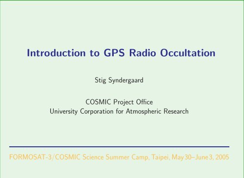
Introduction to GPS Radio Occultation
Stig Syndergaard
COSMIC Project Office
University Corporation for Atmospheric Research
FORMOSAT-3/COSMIC Science Summer Camp, Taipei, May30–June3, 2005

The basics
Topics of lecture
• The GPS radio occultation principle
• GPS observations (what is the signal?)
• Derived products (what comes out of it?)
Inversion of GPS radio occultation data
• From signal to products (next slide)
Advanced topics
• Atmospheric multipath propagation
• Super refraction

Topics of lecture (continued)
Inversion of GPS radio occultation data
• Excess phase → excess Doppler
• Excess Doppler → bending angle
– Correction for Earth’s oblateness
– Ionospheric correction
– Statistical optimization
• Bending angle → refractivity
– The Abel transform (the core of the data inversion)
• Refractivity → pressure, temperature & humidity
Ionospheric data
• Phase differential → total electron content (TEC)
• Total electron content → electron density

The GPS radio occultation principle
GPS = Global Positioning System
LEO = Low Earth Orbiter
α = Bending angle (max ∼2 ◦ )
Signal frequencies: f1 = 1.57542 GHz & f2 = 1.22760 GHz
Refractive index of medium: n ≈ 1+77.6 p e
+3.73×105
T T 2+40.3Ne f 2

Basic GPS occultation observations
Basic measurement is a phase path (meters): L =
a) The Doppler depends on Φ and �v
b) With bending, the Doppler is different
than expected from velocities
only
� LEO
n ds
GPS
Excess phase (path) is defined as: ∆L = L − |�r − �r |
LEO GPS
We are interested in the phase change: excess Doppler = d∆L/dt

The bending effect
Curved signal path through the atmosphere
• The signal path is curved according to Snell’s law because of
changes in the index of refraction along the path
• In a spherically symmetric medium, Snell’s law is replaced by
Bouger’s law:
nr sin ψ = a = constant
ray path
n ( r)−field
r
ψ

The bending effect
Bouger’s law leads to (e.g., Fjeldbo et al. 1971):
α(a) = −2a
� ∞
r0
d ln n/dr
√ n 2 r 2 − a 2 dr
where bending toward the Earth is counted positive and r0 is the
radius at the tangent point: n(r0)r0 = a

Derived data products
Basic assumption: local spherical symmetry
• Bending angle as a function of impact parameter, a (ray asymptote)
– Numerical weather prediction & Climate research
• Refractivity (defined as N = (n−1)×10 6 ) as a function of altitude
– Numerical weather prediction & Climate research
• Temperature, pressure (geopotential height), and humidity profiles
– Atmospheric & Climate research
Ionospheric data
• Total electron content between GPS and LEO
– Input to space weather models
• Electron density as a function of altitude
– Ionospheric research

Data product characteristics
Accuracy of derived refractivity
• Mean accuracy less than 0.5% between 2 and 25 km
• Standard deviation less than 1% between 5 and 25 km
• In the troposphere: Accuracy limited by horizontal gradients
• Above ∼30 km: accuracy limited by thermal and ionospheric noise
• Below ∼2 km: tracking errors may dominate
Vertical resolution
• ∼100 m in lower troposphere, increasing to ∼1.5 km in stratosphere
Ionospheric data
• Accuracy of electron density profiles limited by horizontal gradients
• Vertical resolution determined by sampling rate (∼2 km for 1 Hz data)

L 1,L
A ,A
1
2
2
Satellite orbits &
Spherical symmetry
L 1,L2
Data processing chain
L1 and L2 phase and amplitude
Single path
Radio holographic methods, multipath
α ,α
1 2
Ionospheric correction
L1 and L2 bending angle
High altitude climatology & Abel inversion
L1 and L2 phase
α
Iono−free bending angle
N
Auxiliary meteorological data
Refractivity
T,e,p

excess phase (m)
Excess phase — what does it look like?
3000
2500
2000
1500
1000
500
0
GPS/MET, 1995, doy 174, 1:56 UTC, 16.7S, 171.1E
L1
L2
LC
-500
0 10 20 30 40 50 60 70 80 90
time since start of occultation (s)
excess phase (m)
9
8
7
6
5
4
3
2
1
0
GPS/MET, 1995, doy 174, 1:56 UTC, 16.7S, 171.1E
L1
L2
LC
-1
0 5 10 15 20 25 30
time since start of occultation (s)
• An occultation typically lasts about 1 minute (sometimes more)
• The excess phase can become as large as a few km near the surface
∆LC(t) = f 2 1 ∆L1(t) − f 2 2 ∆L2(t)
f 2 1 − f 2 2
= LC(t) − |�r GPS − �r LEO|

excess phase (m)
Excess phase — what does it look like?
3000
2500
2000
1500
1000
500
0
GPS/MET, 1995, doy 174, 1:56 UTC, 16.7S, 171.1E
L1
L2
LC
-500
0 10 20 30 40 50 60 70 80 90
time since start of occultation (s)
excess phase (m)
0.35
0.3
0.25
0.2
0.15
0.1
0.05
0
GPS/MET, 1995, doy 174, 1:56 UTC, 16.7S, 171.1E
L1
L2
LC
-0.05
0 0.5 1 1.5 2
time since start of occultation (s)
• An occultation typically lasts about 1 minute (sometimes more)
• The excess phase can become as large as a few km near the surface
∆LC(t) = f 2 1 ∆L1(t) − f 2 2 ∆L2(t)
f 2 1 − f 2 2
= LC(t) − |�r GPS − �r LEO|

excess Doppler (m/s)
Excess Doppler — what does it look like?
140
120
100
80
60
40
20
0
GPS/MET, 1995, doy 174, 1:56 UTC, 16.7S, 171.1E
L2
L1 ∆D = d∆L
dt
-20
0 10 20 30 40 50 60 70 80 90
time since start of occultation (s)
Usually smoothing (low
pass filtering) is applied
to the excess phase before
the excess Doppler is
derived (not in this plot,
though)
• L2 signal is affected by Anti-Spoofing (encryption of the P-code)
which leads to a low signal-to-noise ratio, in turn leading to tracking
errors in the lower troposphere (L2 not used in lower troposphere)

Excess Doppler → bending angle
• Having satellite positions & velocities (from precise orbit determination)
• Having the excess Doppler (from observations)
• Assuming spherical symmetry then determines the impact parameter, a,
and subsequently the bending angle, α

∆D(t) →
Excess Doppler → bending angle
∆D + ˙ �
RLG − | ˙¯ RL| cos ϕ(a) − | ˙¯
�
RG| cos χ(a) = 0
�
a
ϕ(a) = ζ − arcsin
| ¯ �
RL|
�
a
χ(a) = (π − η) − arcsin
| ¯ �
RG|
�
a
α = Θ − arccos
| ¯ � �
a
− arccos
RL|
| ¯ �
RG|
(e.g., Melbourne et al. 1994)
→ α(a)
• Bending angle derived from Doppler is used in the stratosphere
and perhaps upper troposphere, but not in the lower troposphere
• In the moist lower troposphere, multipath propagation may be
present, and more advanced methods has to be used to derive
the bending angle (more about this later)

Correction for Earth’s oblateness
• The Earth is slightly oblate (elliptical) such that the center of curvature
does not match the center of the Earth in general
• The center of curvature varies with position on the Earth and the orientation
of the occultation plane
(Syndergaard 1998)
• α and a are estimated with respect to the center of a circle in the
occultation plane that best fits the ellipsoid near the tangent point

Ionospheric correction of bending angles
Consider approximate equations for the L1 and L2 bending angles:
� ∞
d
�
αi(a) ≈ −2a 10
a dx
−6 Nn − 40.3
f 2 �
dx
Ne √
i x2 − a2 The ionosphere-free bending angle is formed from the derived bending
angles at the same impact parameter (Vorob’ev and Krasil’nikova
1994):
α(a) = f 2 1 α1(a) − f 2 2 α2(a)
f 2 1 − f 2 2
≈ −2a
� ∞
a
√ x 2 − a 2
10 −6(dNn/dx)dx
• Ionospheric correction of phases assumes that the L1 and L2
signal paths are identical (but the ionosphere is dispersive)
• Ionospheric correction of bending angles at equal impact parameters
ensures that the involved L1 and L2 signal paths are close
to each other near the tangent point (and that is an advantage)

Statistical optimization
• Formally, we need bending angles to infinite altitudes in order
to derive the refractivity (of course we don’t have that)
• Bending angles are contaminated with thermal noise and residual
noise from ionospheric turbulence
• Fractionally the noise increases exponentially with altitude
rendering the bending angle useless at some altitude and above
”Optimal” estimation of bending angle:
˜α(a) = αmodel(a) +
σ 2 model
σ 2 model + σ2 obs
[α(a) − αmodel(a)]
αmodel is estimated from a climatological model
σobs may be evaluated from the data above the stratosphere
σmodel is usually set to a fixed number (20%)

height of ray asymptote (km)
Bending angle — what does it look like?
120
100
80
60
40
20
GPS/MET, 1995, doy 174, 1:56 UTC, 16.7S, 171.1E
Ionosphere-free bending angle
0
-0.005 0 0.005 0.01 0.015 0.02 0.025 0.03 0.035
bending angle (rad)
height of ray asymptote (km)
10
9
8
7
6
5
4
3
GPS/MET, 1995, doy 174, 1:56 UTC, 16.7S, 171.1E
Ionosphere-free bending angle
2
0 0.01 0.02 0.03 0.04
bending angle (rad)
• Bending is significant only below ∼25 km (but still important above)
• The bending angle may be as large as 0.035 rad (2 ◦ ) near the surface
• In the lower troposphere, moisture variations causes large fluctuations in
the bending angle (multipath propagation, which I will get to shortly)

height of ray asymptote (km)
Bending angle — what does it look like?
120
100
80
60
40
20
GPS/MET, 1995, doy 174, 1:56 UTC, 16.7S, 171.1E
Ionosphere-free bending angle
0
-0.005 0 0.005 0.01 0.015 0.02 0.025 0.03 0.035
bending angle (rad)
height of ray asymptote (km)
120
110
100
90
80
70
60
50
40
GPS/MET, 1995, doy 174, 1:56 UTC, 16.7S, 171.1E
L1
L2
Ionosphere-free
Statistically optimized
0 5e-05 0.0001 0.00015 0.0002
bending angle (rad)
• Bending is appreciable only below ∼25 km (but still important above)
• The bending angle may be as large as 0.035 rad (2 ◦ ) near the surface
• In the lower troposphere, moisture variations causes large fluctuations in
the bending angle (multipath propagation, which I will get to shortly)

Bending angle → refractivity
� ∞
α(a) = −2a
α(a)
↓
Abel integral transform (e.g., Fjeldbo 1971)
r0
d ln n/dr
√
n2r2 − a2 dr ⇐⇒ n(r0)
� � ∞
1
= exp
π a
r0 = a
n(r0)
, N(r0) = 10 6 × (n(r0) − 1)
↓
N(r)
α(x)
√
x2 − a2 dx
�
• The Abel integral transform relies on the assumption of spherical
symmetry
• It provides a simple and unique solution to an otherwise underdetermined
inverse problem
• In practice the integration is performed to some high altitude
where the bending angle can be neglected (above 100 km)

Refractivity — what does it look like?
tangent point altitude (km)
40
35
30
25
20
15
10
5
GPS/MET, 1995, doy 174, 1:56 UTC, 16.7S, 171.1E
Abel-retrieved refractivity
0
0 50 100 150 200 250 300 350
refractivity (N-units)
• The inverse Abel integral (going from bending angle to refractivity)
acts as a low pass filter, somewhat similar to the operator
of a half integration
• Possibly the product that will be assimilated at most NWP centers
in the near future

Refractivity → pressure & temperature
Refractivity equation:
N ≈ 77.6 p
T
+ 3.73 × 105 e
T 2
• Two terms: a dry (or hydrostatic) term and a wet term
• The wet term can be neglected at temperatures less than
∼240 K (i.e., at few kilometers above the surface at high latitudes
and above ∼10 km at tropical latitudes)
Neglecting the wet term:
N(r) →
p
N = 77.6
T
, p = ρRdT
dp
= −ρg
dz
, z = r − rcurv
→ p(z), T (z)

Temperature — what does it look like?
altitude (km)
45
40
35
30
25
20
15
10
5
0
GPS/MET, 1995, doy 174, 1:56 UTC, 16.7S, 171.1E
GPS/MET "dry"
ECMWF
NCEP
-80 -60 -40 -20 0 20 40
temperature ( o C)
• The temperature derived by neglecting water vapor is called the
”dry temperature”
• The dry temperature significantly underestimates the actual
temperature in the lower moist troposphere

Deriving water vapor pressure
Two common ways of deriving water vapor:
1. include additional information about the actual temperature
profile and solve directly for water vapor (iterative procedure)
2. One-dimensional variational technique optimally combining the
refractivity profile with information from an NWP model
Method number 1:
e = T 2 N − 77.6(pd + e)/T
3.73 × 10 5
N(z), Tapriori(z)
↓
,
d(pd + e)
= −(ρd + ρw)g
dz
pd = ρdRdT , e = ρwRwT
↓
e(z), pd(z)

Deriving water vapor pressure
Method number 2 (variational retrieval):
• Include information about errors in a priori temperature, pressure
and water vapor, as well as errors in the observed refractivity
N(z), Tapriori(z), papriori(z), eapriori(z)
↓
Minimizing the following cost function:
J(x) = (x − xb) T B −1 (x − xb) + (Nobs − N(x)) T R −1 (Nobs − N(x))
x is the state vector to be solved for
xb is the a priori state vector
N(x) is the refractivity equation
B is the a priori error covariance matrix
R is the observation + representativeness error covariance matrix
↓
T (z), p(z), e(z)

Water vapor — what does it look like?
altitude (km)
12
10
8
6
4
2
GPS/MET, 1995, doy 174, 1:56 UTC, 16.7S, 171.1E
GPS/MET using NCEP
1DVar using ECMWF
ECMWF
NCEP
0
0 5 10 15 20 25 30
water vapor pressure (hPa)
• The two methods result in almost the same water vapor profiles
• 1DVar retrieval is presumably the most accurate, since it includes
most information, but the very high vertical resolution is lost

A few words about ionospheric data
• Bending throughout (most of) the ionosphere can be ignored
Definition of total electron content: TEC = 10 −16
� LEO
Neds
Our observations: Li =
L1(t), L2(t)
↓
TEC = L1 − L2
40.3 × 10 16
↓
TEC(r)
� LEO
(10 −6 Nn− 40.3
f 2 Ne)ds
i
f 2 1 f 2 2
f 2 1 − f 2 2
GPS
Ne(r0) = 1016
π
• dTEC/dr is proportional to the bending angle
GPS
TEC(r)
↓
� rLEO
r0
↓
Ne(r)
dTEC/dr
�
r2 − r2 dr
0

Ionospheric profiles — what do they look like?
altitude (km)
800
700
600
500
400
300
200
100
GPS/MET, 1995, doy 174, 1:56 UTC, 16.7S, 171.1E
Trans-ionospheric (sub-orbit) TEC
0
0 20 40 60 80 100 120 140
total electron content (TECU)
altitude (km)
800
700
600
500
400
300
200
100
GPS/MET, 1995, doy 174, 1:56 UTC, 16.7S, 171.1E
Ionospheric electron density
0
0 100000 200000 300000 400000 500000
electron density (cm -3 )
• TEC calibrated with positive elevation angle data (Schreiner et al. 1999)
• Retrieval of Ne is based on the assumption of spherical symmetry
• The spherical symmetry assumption may result in large under-estimation
or over-estimation of electron density in the lower part of profiles

ADVANCED TOPICS
• Atmospheric multipath propagation
• Super refraction

Multipath propagation
Atmospheric multipath propagation refers to the situation where there are
more than one signal path (Fermat’s principle) between the transmitter
(GPS) and the receiver (LEO)
(Gorbunov 2002)
• Multipath propagation is a result of sharp vertical refractivity gradients
varying rapidly with height (due to the water vapor term)
• Multipath propagation can be expected in the lower troposphere in regions
with large amounts of water vapor

Multipath propagation
(Beyerle et al. 2003)
• Multipath propagation results in interference in the phase measurements
• We need to disentangle the multipath because the Abel transform is
based on the assumption of single ray propagation
• Radio-holographic methods basically transform the measured signal from
geometrical space to impact parameter space where multipath is absent

excess phase (m)
3000
2500
2000
1500
1000
500
Phase & amplitude → bending angle
GPS/MET, 1995, doy 174, 1:56 UTC, 16.7S, 171.1E
L1
0
0 10 20 30 40 50 60 70 80 90
time since start of occultation (s)
Signal-to-noise ratio (volts/volt)
1200
1000
800
600
400
200
GPS/MET, 1995, doy 174, 1:56 UTC, 16.7S, 171.1E
CA SNR
0
0 10 20 30 40 50 60 70 80 90
time since start of occultation (s)
• Both phase and amplitude is used in radio-holographic methods
A exp(ik∆L1) →
Back propagation (Gorbunov 1998)
Sliding spectrum (Sokolovskiy 2001)
Canonical transform (Gorbunov 2002)
Full spectrum inversion (Jensen et al. 2003)
etc.
→ α1(a)

excess phase (m)
3000
2500
2000
1500
1000
500
Phase & amplitude → bending angle
GPS/MET, 1995, doy 174, 1:56 UTC, 16.7S, 171.1E
L1
0
0 10 20 30 40 50 60 70 80 90
time since start of occultation (s)
Signal-to-noise ratio (volts/volt)
1200
1000
800
600
400
200
GPS/MET, 1995, doy 174, 1:56 UTC, 16.7S, 171.1E
CA SNR
0
0 10 20 30 40 50 60 70 80 90
time since start of occultation (s)
• Both phase and amplitude is used in radio-holographic methods
A exp(ik∆L1) →
Back propagation (Gorbunov 1998)
Sliding spectrum (Sokolovskiy 2001)
Canonical transform (Gorbunov 2002)
Full spectrum inversion (Jensen et al. 2003)
etc.
→ α1(a)

Bending angle — different methods
height of ray asymptote (km)
10
9
8
7
6
5
4
3
2
GPS/MET, 1995, doy 174, 1:56 UTC, 16.7S, 171.1E
Doppler
Back propagation
Sliding spectrum
Canonical transform
Full spectrum inversion
0 0.01 0.02 0.03 0.04
L1 bending angle (rad)
• Deriving the bending angle in the lower troposphere using Doppler may
result in multivalued bending angle as a function of impact parameter
• Different radio-holographic methods give almost the same answer, but
Full Spectrum Inversion (FSI) is at present the most commonly used

Super refraction
Super refraction refers to the situation when the bending becomes so large
(locally) that the curvature of a ray exceeds the curvature of the atmosphere
Critical refraction point:
dN/dr ≈ −157 N-units/km
Super refraction:
dN/dr < −157 N-units/km
Ducting layer in this figure:
Between 1.5 and 2 km
• No ray path connecting satellites can exist with a tangent point altitude
within a layer just below the critical refraction point
• A signal launched horizontally within this layer will be trapped or ducted

(Sokolovskiy 2003)
Super refraction
• Super refraction may happen near the top
of the moist marine boundary layer
• Bending angle theoretically goes to infinity
at the critical refraction point
• Applying the Abel transform gives a negative
refractivity bias below the critical refraction
point
• There is in fact an infinite number of different
refractivity profiles corresponding to
identical bending angle profiles
• Super refraction is largely an unsolved
problem for GPS radio occultation
– Super refraction is not easy to detect in the data
(poses a problem for NWP)
– We do not really know how to handle it properly even
if we could detect it

References and suggested reading
Beyerle, G., M. E. Gurbunov, and C. O. Ao, 2003: Simulation studies of GPS radio occultation measurements.
Radio Sci., 38, 1084, doi:10.1029/2002RS002800.
Fjeldbo, G., A. J. Kliore, and V. R. Eshleman, 1971: The neutral atmosphere of Venus as studied with the
Mariner V radio occultation experiments. Astron. J., 76, 123–140.
Gorbunov, M. E., 2002: Canonical transform method for processing radio occultation data in the lower
troposphere. Radio Sci., 37, 1076, doi:10.1029/2000RS002592.
Gorbunov, M. E., 2002: Ionospheric correction and statistical optimization of radio occultation data. Radio
Sci., 37, 1084, doi:10.1029/2000RS002370.
Gorbunov, M. E., 2002: Radio-holographic analysis of microlab-1 radio occultation data in the lower
troposphere. J. Geophys. Res., 107, doi:10.1029/2000JD000889.
Gorbunov, M. E. and A. S. Gurvich, 1998: Algorithms of inversion of Microlab-1 satellite data including
effects of multipath propagation. Int. J. Remote Sens., 19, 2283–2300.
Healy, S. B., 2001: Smoothing radio occultation bending angles above 40 km. Ann. Geophys., 19, 459–468.
Healy, S. B. and J. R. Eyre, 2000: Retrieving temperature, water vapour and surface pressure information
from refractive-index profiles derived by radio occultation: A simulation study. Quart. J. Roy. Meteorol.
Soc., 126, 1661–1683.
Jensen, A. S., M. S. Lohmann, H.-H. Benzon, and A. S. Nielsen, 2003: Full spectrum inversion of radio
occultation signals. Radio Sci., 38, 1040, doi:10.1029/2002RS002763.
Kuo, Y.-H., T.-K. Wee, S. Sokolovskiy, C. Rocken, W. Schreiner, D. Hunt, and R. A. Anthes, 2004: Inversion
and error estimation of GPS radio occultation data. J. Meteorol. Soc. Japan, 82, 507–531.

References and suggested reading
Kursinski, E. R. and G. A. Hajj, 2001: A comparison of water vapor derived from GPS occultations and
global weather analyses. J. Geophys. Res., 106, 1113–1138.
Kursinski, E. R., G. A. Hajj, S. S. Leroy, and B. Herman, 2000: The GPS radio occultation technique.
Terrestrial, Atmospheric and Oceanic Sciences, 11, 53–114.
Melbourne, W. G., et al., 1994: The application of spaceborne GPS to atmospheric limb sounding and global
change monitoring. JPL-Publication 94-18, Jet Propulsion Laboratory, California Institute of Technology,
Pasadena, California.
Schreiner, W. S., S. V. Sokolovskiy, C. Rocken, and D. C. Hunt, 1999: Analysis and validation of GPS/MET
radio occultation data in the ionosphere. Radio Sci., 34, 949–966.
Sokolovskiy, S., 2003: Effect of superrefraction on inversions of radio occultation signals in the lower
troposphere. Radio Sci., 38, 1058, doi:10.1029/2002RS002728.
Sokolovskiy, S. V., 2001: Modeling and inverting radio occultation signals in the moist troposphere. Radio
Sci., 36, 441–458.
Syndergaard, S., 1998: Modeling the impact of the Earth’s oblateness on the retrieval of temperature and
pressure profiles from limb sounding. J. Atmos. Solar-Terr. Phys., 60, 171–180.
Vorob’ev, V. V. and T. G. Krasil’nikova, 1994: Estimation of the accuracy of the atmospheric refractive
index recovery from Doppler shift measurements at frequencies used in the NAVSTAR system. Physics of the
Atmosphere and Ocean, 29, 602–609.