Validation of a real-time markerless tracking system - American ...

INTRODUCTION
Validation of a real-time markerless tracking system for clinical gait analysis
- ad hoc results -
1 Kai Daniel Oberländer, 1 Gert-Peter Brüggemann
Institute of Biomechanics and Orthopaedics, German Sport University Cologne, Germany
email: k.oberlaender@dshs-koeln.de
Gait analysis in clinical applications is generally
carried out using a retro-reflective maker based
(MB) approach with reconstruction and calculations
of a subject’s 3-dimensional kinematics and kinetics
in the laboratory space. An expert spends a
considerable amount of time identifying anatomical
landmarks by palpation and attaching markers on
the skin. For this purpose, participants are often
asked to remove their clothing, resulting in an
uncomfortable situation. Motion analysis
techniques, which are less time consuming,
contactless, require fewer skills, and do not disturb
the subject, would be favorable in clinical
applications. Several markerless (ML) tracking
techniques have been recently presented and may
play an important role in addressing this topic [1,
2]. In order to identify the applicability and
accuracy of an ML-tracking in clinical gait analysis,
we compare a state-of-the-art ML-system with both
an MB approach and the internal sensor output of a
knee joint prosthesis, by simultaneously acquiring
the same walking path.
METHODS
A male subject with a left-leg prosthesis (Genium,
Otto Bock, Germany) participated in the study. The
subject walked at a self-selected speed over a
distance of 6 m. In order to get relevant
information, fifteen gait cycles of the subject’s left
leg were analyzed. Kinematic data for the MBsystem
were recorded using a 12 infrared camera
system operating at 100 Hz (VICON TM , Oxford,
UK). For the ML-system category, we selected
BioStage (Organic Motion Inc., NYC, USA) due to
its commercial availability for clinical application.
Post-processing was carried out using The
MotionMonitor® (IST, Inc., Chicago, USA). The
internal sensors of the Genium leg prostheses (GE)
operate at 50 Hz and measure kinematic and kinetic
parameters. Joint angle calculations for the MB-
System were performed using a self-devised
optimized soft tissue deformation model for lower
extremities, realized in MATLAB (xxx,xxx,xxx)
[3]. The BioStage system uses an internal full body
model, based on simulated joint constraints. Its
kinematic output was analyzed with The
MotionMonitor® software by using the same angle
conventions as in the MB-model. The GE-system
measures the knee flexion angle with internal
sensors and exports the data via WiFi. To ensure
comparable results of the systems, all joint angles
were normalized to a static reference.
Synchronization was realized by heel-strike events,
using forceplate information in the MB- and MLsystems
as well as reported force data of the GEsystem.
Gait cycles were normalized to 100%. For a
simplified notation, we define two sets:
J= {ankle joint, knee joint, hip joint}
S={MB, ML, GE}
The average joint angles over the 15 gait cycles
were calculated as follows:
u k −1 15 u k
α = 15 ∗∑
β j with k ∈ J ; u ∈ S
j=1
where the subscript j refers to the j th gait cycle of the
joint angle β. In order to account for the offsets
between two systems the absolute difference of the
mean value of the average angles ( u α k ) were
calculated:
Δ u,v α k = u α k − v α k with u, v ∈ S; u≠v ; k ∈J
In order to quantify the differences between the
systems we calculated the root mean square
deviation (RMSD) as well as the normalized root
mean square deviation (nRMSD):

u,v RMSD k =
∑
u k v k ( α i − α i ) 2
n
i=1
n
( ( ) ) −1
u,v k u,v k u k
nRMSD = RMSD ∗ max( α i ) − min v k
α i
where the subscript i refers to the i th frame. Pattern
differences between the systems were quantified
with Spearman’s correlation coefficient:
u,v ρ k = spear( u α k , v α k )
where spear is a symbolic for the entire equation.
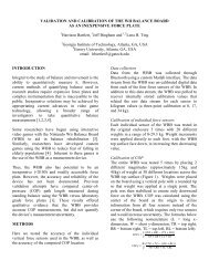
RESULTS AND DISCUSSION
The average sagittal joint angles of the lower
extremity during the gait cycles, estimated by the
MB-, ML-system, and the GE- system for the knee
joint, are reported in Fig. 1. The absolute difference
of the mean value (Δα), the RMSD, the nRMSD
and Spearman’s ρ are reported in Tab. 1. The results
indicate a good alignment of the ML-system
compared to the MB-system as well as to the GEsystem
for the hip (nRMSD=0.04) and knee flexion
(nRMSD=0.05). During the stance phase the ankle
angle comparison showed a similar movement
pattern, to the exception of an overshoot in the MLsystem
of approximately 5° in the first maximum
and minimum, compared to the MB-system. In the
swing phase the ML-system showed a divergent
pattern compared to the ankle angle results of the
MB-system.
CONCLUSIONS
In this report, we presented ad-hoc results of our
validation study to identify the applicability and
accuracy of a ML-system for clinical gait analysis.
The results indicate that ML-systems may play an
important role to address the above described
restrictions of MB-systems due to a good alignment
of the hip and knee angle results. Further
investigation is needed to identify secondary plane
kinematics.
REFERENCES
1.Corazza S., et al Annals of Biomedical Engineer-
ing 34:1019–29, 2006
2.Chu C.W. Proc of IEEE Computer Society
Conference on Computer Vision and Pattern
Recognition, Madison, USA, 2003
3.Oberländer K.D., et al IFMBE Proc of 15. Nordic-
Baltic Conference on Biomedical Engineering and
Medical Physics, Aalbourg, Denmark, 2011
Table 1: Root mean square derivation (RMSD), normalized RMSD (nRMSD), absolute difference of the mean
values (Δα) and Spearman’s correlation coefficient (p) are reported between results of the three systems.
MB vs. ML GE vs. ML GE vs. MB
ankle angle knee angle hip angle knee angle knee angle
Δα 0.26 0.9 0.6 0.9 0.0
RMSD 2.5 3.4 1.9 3.4 1.0
nRMSD 0.19 0.05 0.04 0.05 0.01
ρ 0.89 0.93 1.00 0.94 1.00
Figure 1: Average joint angles of 15 gait cycles for the lower extremity normalized to 100 %. (A: ankle angle;
B: knee angle; C: hip angle; shadowed: standard deviation)