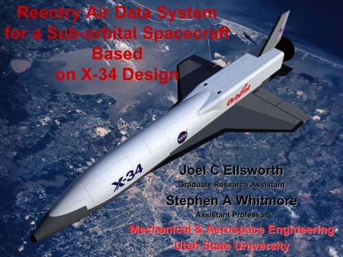
Reentry Air Data System for a Sub-orbital Spacecraft Based on X-34 ...

<strong>Reentry</strong> <strong>Air</strong> <strong>Data</strong> <strong>System</strong>
<strong>for</strong> a <strong>Sub</strong>-<strong>orbital</strong> <strong>Spacecraft</strong>
2007 USU Industry Day
<strong>Based</strong>
on X-34 Design
Joel C Ellsworth
Graduate Research Assistant
Stephen A Whitmore
Assistant Professor
Mechanical & Aerospace Engineering
1
Utah State University

2007 USU Industry Day
Background
• Several companies have been <strong>for</strong>mulated during the past
decade with the intention of developing a sup-<strong>orbital</strong> space
tourism market. These companies include Okalahoma City
based Rocketplane-Kistler, Roswell New Mexico based
Virgin Galactic, and San Diego based Benson Space
Company among others.
• Most designs are intended to glide back to earth after
using a rocket engine to boost themselves out of the
atmosphere.
2

2007 USU Industry Day
Background cont.
• Regardless of the particular design features or mission
operations these trans-atmospheric vehicles are generally
more aircraft than spacecraft
• <strong>Air</strong>-mass reference measurements are required <strong>for</strong> flightcritical
sub-systems such as inertial guidance, inner and
outer-loop flight control, terminal area energy
management, and on-launch winds biasing to keep the
angles of attack and sideslip within prescribed limits.
• Knowledge of the wind-relative vehicle state parameters -dynamic
pressure, Mach number, angle-of-attack and -
sideslip, and surface winds – are especially critical <strong>for</strong> the
landing phase <strong>for</strong> energy management and runway
alignment.
3

Why use the X-34 as a Baseline Vehicle?
• The X-34 was chosen <strong>for</strong> this
study because it incorporates
many of the features needed
by a commercial sub<strong>orbital</strong>
tourist spaceflight system.
• The X-34 aerodynamic
database was developed using
public dollars and is available
in the public domain.
• For this design study a typical
X-34 trajectory was used to
generate simulated nosecap
surface pressure values based
on wind-tunnel derived
calibration models.
2007 USU Industry Day
4

2007 USU Industry Day
X-34 Trajectory
5

2007 USU Industry Day
Why Develop a New <strong>System</strong>?
• High temperatures and
dynamic pressures
associated with
attached shockwaves
will destroy pitot probes
and directional vanes
• Heating proportional to
q&
heat
∝
1
R
le
6

2007 USU Industry Day
Solution:
• Place pressure sensors
behind detached
shockwave
• Blending Hypersonic
(Modified Newtonian) flow
with a potential flow
solution allows an
algorithm to determine
the flight data state.
7

2007 USU Industry Day
Flow Model
• The FADS algorithm uses the pressures measured
by a matrix (at least five) of flush mounted pressure
ports to produce a full air data state.
2 2
( ) cos sin
p = qc ⎡
⎣ + ⎤
⎦+
p
Cp
Cp
FADS flow model <strong>for</strong>
a spherical nosecap
2 θ θ ε θ ∞
( )
( )
( θ )
p − p
5
= = cos − sin
qc
4
∞ 2 2
θ θ θ
( θ )
p − p
= =
qc
cos
∞ 2
θ θ
Potential flow <strong>for</strong> a sphere
(M 1)
8

2007 USU Industry Day
Pressure Model
• local flow is related to local flow incidence angle, θ,
and port locations (φ, λ) through geometry
⎡cosαcos β⎤ ⎡ cos λ ⎤
V ⋅ R
cosθ = =
⎢
sin β
⎥ ⎢
sinφsin λ
⎥
V R ⎢ ⎥ ⎢ ⎥
⎢⎣sinα cos β ⎥⎦ ⎢⎣cosφsin λ⎥⎦
X FADS =
⎡
⎢
⎢
⎢
⎢
⎣
α ind
β ind
q c 2
p ∞
⎤
⎥
⎥
⎥
⎥
⎦
Τ
cosθi = cosαind cos βind cosφi
+ sin βind sin λisinφi + sinα cos β cosλ sinφ
ind ind i i
9

2007 USU Industry Day
Triples Formulation
• By taking strategic differences of three surface
sensor readings ("triples") the parameters qc 2 , p ∞ ,
and ε, are eliminated.
This yields
where
Γ ik cos 2 θ j +Γ ji cos 2 θ k +Γ kj cos 2 θ i = 0
Γ ik = p i − p k , Γ ji = p j − p i , Γ kj = p k − p j
10

2007 USU Industry Day
Angle of Attack solution
• The parameter αind
can be de-coupled from βind
by
using only pressures triples aligned along a vertical
meridian. The result is a quadratic expression αin
ind
terms 2 of 2tan 2 2 2 2 2
⎣
⎡Γ ik sin φj+Γ ji sin φk+Γ kj sin φi⎦ ⎤tan αind + ⎣
⎡Γ ik cos φj+Γ ji cos φk+Γ kj cos φi⎦
⎤+
2 ⎡
⎣Γ ik cosφjsinφjcosλj+Γ ji cosφksinφkcos λk+Γ kj cosφisinφicosλ ⎤ i ⎦tanαind
= 0
Where the solution is either
o 1
αind ≤ 45 → αind
= tan
2
where
A
⎢
⎣ B ⎥
⎦
−1 ⎡ ⎤
or
o 1 ⎛ −1
⎡ A⎤
⎞
αind ≥ 45 → αind = π tan
2
⎜ −
⎢ B ⎥ ⎟
⎝ ⎣ ⎦ ⎠
2 2 2
A= ⎡
⎣Γ ik sin φj+Γ ji sin φk+Γkjsin φ ⎤ i ⎦
B = ⎡
⎣Γ ik cosφ j sinφjcosλj+Γ ji cosφksinφkcosλk+Γkjcosφisinφicos λ ⎤ i ⎦
11

2007 USU Industry Day
Angle of Sideslip Solution
• Once we know Angle of Attack, we can calculate
Angle of Sideslip using any combination of ports
exclusive of sets with all ports on the vertical
meridian 2
A'tan β + 2B'tanβ + C'=
0
where
a
b
ind ind
( ik
2
j ji
2
k kj
2
i )
( ik j j ji k k kj i i )
( ik
2
j ji
2
k kj
2
i )
A'= Γ b +Γ b +Γ b
B'= Γ a b +Γ a b +Γ ab
C'= Γ a +Γ a +Γ a
= cosα cos λ + sinα sin λ cosφ
( ijk ) ind ( ijk ) ind ( ijk ) ( ijk )
=
sin λ sinφ
( ijk ) ( ijk ) ( ijk )
12

2007 USU Industry Day
Altitude & Mach calculation
• Three unknowns left in system, 5+ pressure
measurements => over determined system.
Solved with pseudo inverse
−1
⎡ ⎡Θ1 1⎤⎤
⎡ ⎡p1⎤⎤ q
⎢ ⎥ ⎢ ⎥
⎡ c ⎤
⎢
2
1 2 n 2 1
⎥ ⎢
1 2
n p
⎥
⎢⎡Θ Θ L Θ ⎤ 2
[ Q] ⎢
Θ
⎥⎥ ⎢⎡Θ Θ L Θ ⎤
[ Q]
⎥
⎢ ⎥ =
⎢ ⎥
⎢ n× n n× n
p 1 1 1
⎥ ⎢
1 1 1
⎥
⎣ ∞ ⎦
⎢⎣ L ⎦ ⎢ M M⎥⎥ ⎢⎣ L ⎦ ⎢ M ⎥⎥
⎢ ⎢ ⎥⎥ ⎢ ⎢ ⎥⎥
⎢⎣ ⎢⎣ Θn
1⎥⎦⎥⎦
⎢⎣ ⎢⎣pn⎥⎦⎥⎦ where
2 2
Θ = cos θ + εsinθ [ Q]
i i i
n× n
⎡q10 L 0 ⎤
⎢
0 q2
0
⎥
⎢
M
= ⎥
⎢ M 0 O 0 ⎥
⎢ ⎥
⎢⎣0 L 0 qn
⎥⎦
This can be simplified to
⎡
⎢
n
∑qi n n
⎤⎡ ⎤
−∑qiΘi⎥⎢∑pq i iΘi⎥ i= 1 i= 1 i=
1
⎢ ⎥⎢ ⎥
n n n
⎢ 2 ⎥⎢ ⎥
− qiΘi qiΘi pq i i
⎡qc⎤ ⎢ ∑ ∑ ⎥⎢ ∑ ⎥
2 ⎣ i= 1 i= 1 ⎦⎣ i=
1 ⎦
⎢ ⎥ =
n n n
2
⎣p∞⎦ ⎛ 2 ⎞⎛ ⎞ ⎛ ⎞
⎜∑qiΘi ⎟⎜∑qi ⎟−⎜∑qiΘi 13 ⎟
⎝ i= 1 ⎠⎝ i= 1 ⎠ ⎝ i=
1 ⎠

Altitude & Mach calculation
• Pressure altitude is a straight<strong>for</strong>ward calculation, or
simple table lookup routine.
• Mach number is more complicated
• <strong>System</strong> must be iterated since the calibration
parameter ε is a function of Mach number
2007 USU Industry Day
14

2007 USU Industry Day
Mach calculation - subsonic
For the subsonic case, Mach number is given by isentropic
flow
M
q
p
c
2
∞
γ −1
⎡ ⎤
2 ⎛qc⎞ γ
2
= ⎢ 1 1⎥
⎜ + ⎟ −
γ −1 ⎢
⎝ p ⎥
∞
⎢
⎠
⎣ ⎥⎦
Supersonic case is solved using the Rayleigh-Pitot equation
γ
γ −1
⎛γ+ 1 2 ⎞
⎜ M ∞ ⎟
2
=
⎝ ⎠
−1
∞ ⎛
1
2γ 1
2 γ −1⎞γ−
M ∞ −
⎜
γ + 1 γ + 1
⎟
⎝ ⎠
15

2007 USU Industry Day
Real Gas Effects
• An “averaged” value <strong>for</strong> γ across the shockwave is
calculated using Eckert’s empirical reference temperature
Tref = T∞ + 1
2 Tawall − T ( ∞)+
0.22( T0 2 − T ) ∞
where Tawal l = T ⎡ 3
∞ 1 + Pr ⎣
⎢
γ − 1
2 M 2
∞
⎤
⎡
⎦
⎥ and T02 = T∞ 1 +
⎣
⎢
P r is the Prandtl number <strong>for</strong> air μC p /κ
γ − 1
2 M 2
∞
• These equations are solved iteratively, with the gas
properties coming from real gas tables
⎤
⎦
⎥
16

No system
Noise
Demonstrat
es solver
consistency
2007 USU Industry Day
X-34 Solver Example - Clean
Alpha Mach
Sideslip Altitude
17

•Sensor Noise
•Random
•Bias
•Lag
•Resolution
•Latency
2007 USU Industry Day
X-34 Solver w/ Sensor Noise
Alpha Mach
Sideslip Altitude
18

2007 USU Industry Day
How do we reduce effect of noise ?
• Relatively Unbiased but noisy FADS data (at
high altitude)
• Relatively clean but biased inertial data from
INS (upper atmospheric winds)
• Design filter to keep desired properties of
each and ignore undesirable properties of
each
19

How do we reduce the effect of noise?
• Complementary Inertial Filters
– In the Laplace domain
– However, the rest of the algorithm is non-continuous, so the
conversion back to the time domain is not a simple one.
– Necessitates usage of a Bi-Linear trans<strong>for</strong>m
2007 USU Industry Day
τ sβ
+ β
β =
τ s + 1
inertial FADS
⎡z−1⎤ 1
s = a
⎢
⇒ β = β + β −β
⎣z+ 1⎥
⎦
⎡z−1⎤ a
⎢ τ + 1
⎣z+ 1⎥
⎦
( )
inertial FADS inertial
20

2007 USU Industry Day
Noise reduction at high altitude
• True airdata at high altitudes can be so deeply
buried in noise that it becomes useless.
– Weight out FADS data and replace it with inertial
– Include in previously derived filter, yielding
⎛Δt⎞ 1−tan⎜ ⎟
2τ
1
βk =
⎝ ⎠
βk−1+ ( βinert −β
)
k inertk−1
⎛Δt ⎞ ⎛Δt ⎞
1+ tan ⎜ ⎟ 1+ tan ⎜ ⎟
⎝2τ ⎠ ⎝2τ ⎠
⎛Δt ⎞
Atan ⎜ ⎟
2τ +
⎝ ⎠ ( β
⎛Δt ⎞
1+ tan⎜ ⎟
⎝2τ ⎠
− β
⎛Δt ⎞
( 1− A)
tan ⎜ ⎟
⎝2τ ⎠
) +
⎛Δt ⎞
1+ tan⎜
⎟
⎝2τ ⎠
β −β
( )
FADS FADS inert inert
k k−1 k k−1
Similar filters <strong>for</strong> AoA, Mach, Altitude
21

•Sensor
Noise
•Random
•Bias
•Lag
•Lag
•Resolutio
n
•Latency
•Inertial Filter
retains salient
features of
FADS data,
but removes
noise
2007 USU Industry Day
X-34 with Inertial Filter & Noise
Alpha Mach
Sideslip Altitude
22

2007 USU Industry Day
FADS <strong>System</strong> Redundancy
• Extra Ports add fail-operational capability as
well as noise reduction
• An additional system can provide complete
redundancy
• <strong>System</strong> health (accuracy) can be monitored
by use of a Chi-squared test on the system
residuals
23

2007 USU Industry Day
χ 2 (Chi-squared) Test
• The Chi-squared value is given by
χ 2
δ p =
n−1
∑
i − 0
And represents the
probability the system has
failed
~> 1-Probability(χ 2 ) yields
the probability the system is
healthy
For redundant systems, the
system with better χ2 value is
used.
( )
pi − qc 2 cos 2θ i + ε sin 2 { ⎡⎣
θi ⎤⎦ + p } ∞
2
σ 2
δ p
24

2007 USU Industry Day
X-34 FADS <strong>System</strong> Structure
25

2007 USU Industry Day
X-34 FADS <strong>System</strong> Hardware cont.
Pressure port locations
<strong>for</strong> the X-34
Pressure port assembly
Ames technology Capabilities and Facilities, Entry <strong>System</strong>s Technologies, NASA
Thermophysics Facilities Branch Fact Sheet, Arc jet Complex , NASA 26
Engineerng Analysis <strong>for</strong> X-34 Thermal Protection <strong>System</strong>, Journal of <strong>Spacecraft</strong> and Rockets

2007 USU Industry Day
Questions?
27

2007 USU Industry Day
Mach Number - Supersonic
• The assumption that γ=1.4, explicitly holds only <strong>for</strong>
Mach numbers up to about 4.0
• For Mach number below 3.0, real-gas effects can be
ignored and a Taylor’s series expansion and reversion of
series can be used to solve explicitly <strong>for</strong> Mach number
M ∞
2 3 4
⎡ ⎤
1 1.428572 - 0.3571429 z - 0.0625 z - 0.025 z - 0.0126172 z
= ⎢ 5 6 9 ⎥
z ⎣ - 0.00715 z - 0.0043458 z - .0087725 z ⎦
where
z =
1.839371
qc2
+ 1
p∞ 28

2007 USU Industry Day
Mach Number - Supersonic
• For the high supersonic and hypersonic regimes, γ ≠ 1.4
and the solution can be found iteratively
( )
F M i
Mi+ 1 Mi
dF( M )
dM
≈ − ⎛ ⎞
⎜ ⎟
⎝ ⎠
i
γ
where
and
γ
γ −1
⎛γ+ 1 2 ⎞
⎜ M ⎟
2
q
=
⎝ ⎠
− −1
1
p
2γ 1
2 γ 1 γ − ∞
⎛ − ⎞
⎜ M − ⎟
⎝γ + 1 γ + 1⎠
c2
( )
F M
⎛γ+ 1 1
2 ⎞γ−⎡
⎤
2γ
M
dF ( M ) ⎜ ⎟ ⎢ ⎥
2
1 2M
=
⎝ ⎠ ⎢ −
⎥
1 2
dM ⎢ 2 ( γ −1) M ⎛ M γ −1
⎞ ⎥
1
2
⎛ M γ −1 ⎞γ−
2γ ( γ 1
2
⎢
γ ⎜ − ⎟ − ) ⎥
⎜ − ⎟ γ + 1 γ + 1
γ 1 γ 1
⎢⎣ ⎝ ⎠ ⎥
⎝ + + ⎠
⎦
29