FIRST-ORDER DIFFERENTIAL EQUATIONS - Mathematics
FIRST-ORDER DIFFERENTIAL EQUATIONS - Mathematics
FIRST-ORDER DIFFERENTIAL EQUATIONS - Mathematics

Create successful ePaper yourself
Turn your PDF publications into a flip-book with our unique Google optimized e-Paper software.
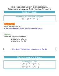
16.1<br />
Chapter<br />
16<br />
<strong>FIRST</strong>-<strong>ORDER</strong><br />
<strong>DIFFERENTIAL</strong> <strong>EQUATIONS</strong><br />
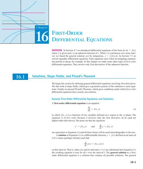
OVERVIEW In Section 4.7 we introduced differential equations of the form dy>dx = ƒ(x) ,<br />
where ƒ is given and y is an unknown function of x.<br />
When ƒ is continuous over some interval,<br />
we found the general solution y(x) by integration, y = 1ƒ(x) dx . In Section 7.5 we<br />
solved separable differential equations. Such equations arise when investigating exponential<br />
growth or decay, for example. In this chapter we study some other types of first-order<br />
differential equations. They involve only first derivatives of the unknown function.<br />
Solutions, Slope Fields, and Picard’s Theorem<br />
We begin this section by defining general differential equations involving first derivatives.<br />
We then look at slope fields, which give a geometric picture of the solutions to such equations.<br />
Finally we present Picard’s Theorem, which gives conditions under which first-order<br />
differential equations have exactly one solution.<br />
General First-Order Differential Equations and Solutions<br />
A first-order differential equation is an equation<br />
dy<br />
dx<br />
= ƒsx, yd<br />
in which ƒ(x, y) is a function of two variables defined on a region in the xy-plane. The<br />
equation is of first order because it involves only the first derivative dy> dx (and not<br />
higher-order derivatives). We point out that the equations<br />
y¿ =ƒsx, yd and d<br />
y = ƒsx, yd<br />
dx<br />
are equivalent to Equation (1) and all three forms will be used interchangeably in the text.<br />
A solution of Equation (1) is a differentiable function y = ysxd defined on an interval<br />
I of x-values (perhaps infinite) such that<br />
d<br />
ysxd = ƒsx, ysxdd<br />
dx<br />
on that interval. That is, when y(x) and its derivative y¿sxd are substituted into Equation (1),<br />
the resulting equation is true for all x over the interval I. The general solution to a firstorder<br />
differential equation is a solution that contains all possible solutions. The general<br />
(1)<br />
16-1
16-2 Chapter 16: First-Order Differential Equations<br />
solution always contains an arbitrary constant, but having this property doesn’t mean a<br />
solution is the general solution. That is, a solution may contain an arbitrary constant without<br />
being the general solution. Establishing that a solution is the general solution may require<br />
deeper results from the theory of differential equations and is best studied in a more<br />
advanced course.<br />
EXAMPLE 1 Show that every member of the family of functions<br />
is a solution of the first-order differential equation<br />
dy<br />
dx = 1 x s2 - yd<br />
on the interval s0, q d,<br />
where C is any constant.<br />
Solution Differentiating y = C>x + 2 gives<br />
Thus we need only verify that for all x H s0, q d,<br />
This last equation follows immediately by expanding the expression on the right-hand side:<br />
Therefore, for every value of C, the function y = C>x + 2 is a solution of the differential<br />
equation.<br />
As was the case in finding antiderivatives, we often need a particular rather than the<br />
general solution to a first-order differential equation y¿ =ƒsx, yd. The particular solution<br />
satisfying the initial condition ysx0d = y0 is the solution y = ysxd whose value is y0 when<br />
x = x0. Thus the graph of the particular solution passes through the point sx0, y0d in the<br />
xy-plane. A first-order initial value problem is a differential equation y¿ =ƒsx, yd<br />
whose solution must satisfy an initial condition ysx0d = y0.<br />
EXAMPLE 2 Show that the function<br />
is a solution to the first-order initial value problem<br />
Solution The equation<br />
dy<br />
dx<br />
- C<br />
x 2 = 1 x c2 - aC x<br />
1 x c2 - a C x + 2b d = 1 x a- C x<br />
dy<br />
dx<br />
y = C x<br />
d<br />
= C<br />
dx a1x b + 0 =-C . 2 x<br />
y = sx + 1d - 1<br />
3 ex<br />
= y - x, ys0d = 2<br />
3 .<br />
dy<br />
dx<br />
+ 2<br />
= y - x<br />
+ 2b d.<br />
is a first-order differential equation with ƒsx, yd = y - x.<br />
b =-C . 2 x
⎛<br />
⎝<br />
0, 2<br />
3<br />
⎛ ⎝<br />
2<br />
1<br />
–4 –2 2 4<br />
–1<br />
–2<br />
–3<br />
–4<br />
y<br />
y � (x � 1) � ex 1<br />
3<br />
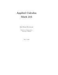
FIGURE 16.1 Graph of the solution<br />
to the differential<br />
equation with initial<br />
condition ys0d = (Example 2).<br />
2<br />
y = sx + 1d -<br />
dy>dx = y - x,<br />
3<br />
1<br />
3 ex<br />
x<br />
On the left side of the equation:<br />
dy<br />
dx<br />
= d<br />
dx<br />
On the right side of the equation:<br />
The function satisfies the initial condition because<br />
ys0d = csx + 1d - 1<br />
3 ex d = 1 -<br />
x = 0<br />
1<br />
3<br />
The graph of the function is shown in Figure 16.1.<br />
Slope Fields: Viewing Solution Curves<br />
16.1 Solutions, Slope Fields, and Picard’s Theorem 16-3<br />
ax + 1 - 1<br />
3 ex b = 1 - 1<br />
3 ex .<br />
y - x = sx + 1d - 1<br />
3 ex - x = 1 - 1<br />
3 ex .<br />
= 2<br />
3 .<br />
Each time we specify an initial condition ysx0d = y0 for the solution of a differential equation<br />
y¿ =ƒsx, yd, the solution curve (graph of the solution) is required to pass through the<br />
point sx0, y0d and to have slope ƒsx0, y0d there. We can picture these slopes graphically by<br />
drawing short line segments of slope ƒ(x, y) at selected points (x, y) in the region of the<br />
xy-plane that constitutes the domain of ƒ. Each segment has the same slope as the solution<br />
curve through (x, y) and so is tangent to the curve there. The resulting picture is called a<br />
slope field (or direction field) and gives a visualization of the general shape of the solution<br />
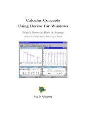
curves. Figure 16.2a shows a slope field, with a particular solution sketched into it in<br />
Figure 16.2b. We see how these line segments indicate the direction the solution curve<br />
takes at each point it passes through.<br />
4<br />
2<br />
–4 –2 0 2 4<br />
–2<br />
–4<br />
y y<br />
4<br />
2<br />
x x<br />
–4 –2 0 2 4<br />
–2<br />
–4<br />
(a) (b)<br />
FIGURE 16.2 (a) Slope field for (b) The particular solution<br />
curve through the point a0, (Example 2).<br />
2<br />
3 b<br />
dy<br />
= y - x.<br />
dx<br />
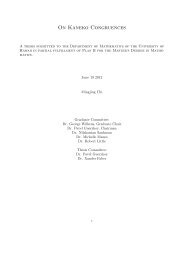
Figure 16.3 shows three slope fields and we see how the solution curves behave by<br />
following the tangent line segments in these fields.<br />
⎛<br />
⎝<br />
3<br />
⎛ ⎝0, 2
16-4 Chapter 16: First-Order Differential Equations<br />
–5<br />
(–5, –1)<br />
–1<br />
5<br />
5<br />
1<br />
–5<br />
y<br />
(7, 5.4)<br />
(5, 1)<br />
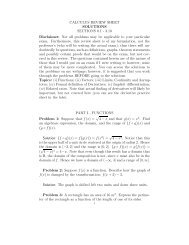
FIGURE 16.4 The graph of the solution<br />
y = (x>5) to the initial value problem in<br />
Example 3. Another solution is y = 0.<br />
5<br />
x<br />
(a) y' � y � x2 2xy<br />
(b) y' � –<br />
2 1 � x<br />
Constructing a slope field with pencil and paper can be quite tedious. All our examples<br />
were generated by a computer.<br />
The Existence of Solutions<br />
A basic question in the study of first-order initial value problems concerns whether a solution<br />
even exists. A second important question asks whether there can be more than one solution.<br />
Some conditions must be imposed to assure the existence of exactly one solution,<br />
as illustrated in the next example.<br />
EXAMPLE 3 The initial value problem<br />
has more than one solution. One solution is the constant function for which the<br />
graph lies along the x-axis. A second solution is found by separating variables and integrating,<br />
as we did in Section 7.5. This leads to<br />
y = a .<br />
x<br />
5 b<br />
dy<br />
y(0) = 0<br />
dx<br />
y(x) = 0<br />
5<br />
= y 4>5 ,<br />
The two solutions and y = (x>5) both satisfy the initial condition y(0) = 0<br />
(Figure 16.4).<br />
We have found a differential equation with multiple solutions satisfying the same initial<br />
condition. This differential equation has even more solutions. For instance, two additional<br />
solutions are<br />
5<br />
y = 0<br />
y = •<br />
0, for x … 0<br />
a x<br />
5 b<br />
5<br />
, forx70 (c) y' � (1 � x)y � x<br />
2<br />
FIGURE 16.3 Slope fields (top row) and selected solution curves (bottom row). In computer<br />
renditions, slope segments are sometimes portrayed with arrows, as they are here. This is not to<br />
be taken as an indication that slopes have directions, however, for they do not.
and<br />
16.1 Solutions, Slope Fields, and Picard’s Theorem 16-5<br />
y = • .<br />
ax<br />
5 b<br />
5<br />
, forx…0 0, for x 7 0<br />
In many applications it is desirable to know that there is exactly one solution to an initial<br />
value problem. Such a solution is said to be unique. Picard’s Theorem gives conditions<br />
under which there is precisely one solution. It guarantees both the existence and uniqueness<br />
of a solution.<br />
THEOREM 1—Picard’s Theorem Suppose that both ƒ(x, y) and its partial<br />
derivative 0ƒ>0y are continuous on the interior of a rectangle R, and that (x0, y0) is<br />
an interior point of R. Then the initial value problem<br />
dy<br />
dx<br />
= ƒ(x, y) , y(x0) = y0<br />
(2)<br />
has a unique solution y � y(x) for x in some open interval containing x0.<br />
The differential equation in Example 3 fails to satisfy the conditions of Picard’s Theorem.<br />
Although the function from Example 3 is continuous in the entire xy-plane,<br />
the partial derivative 0ƒ>0y = (4>5) y fails to be continuous at the point (0, 0) specified<br />
by the initial condition. Thus we found the possibility of more than one solution to the<br />
given initial value problem. Moreover, the partial derivative 0ƒ>0y is not even defined<br />
where y = 0.<br />
However, the initial value problem of Example 3 does have unique solutions<br />
whenever the initial condition y(x0) = y0 has y0 Z 0.<br />
-1>5<br />
ƒ(x, y) = y 4>5<br />
Picard’s Iteration Scheme<br />
Picard’s Theorem is proved by applying Picard’s iteration scheme, which we now introduce.<br />
We begin by noticing that any solution to the initial value problem of Equations (2)<br />
must also satisfy the integral equation<br />
because<br />
y(x) = y0 + ƒ(t, y(t)) dt<br />
Lx0<br />
x<br />
Lx0<br />
dy<br />
dt = y(x) - y(x0).<br />
dt<br />
The converse is also true: If y(x) satisfies Equation (3), then y¿ =ƒ(x, y(x)) and y(x0) = y0.<br />
So Equations (2) may be replaced by Equation (3). This sets the stage for Picard’s interation<br />
x<br />
(3)
16-6 Chapter 16: First-Order Differential Equations<br />
method: In the integrand in Equation (3), replace y(t) by the constant y0,<br />
then integrate and<br />
call the resulting right-hand side of Equation (3) y1(x):<br />
This starts the process. To keep it going, we use the iterative formulas<br />
The proof of Picard’s Theorem consists of showing that this process produces a sequence of<br />
functions {yn(x)} that converge to a function y(x) that satisfies Equations (2) and (3) for<br />
values of x sufficiently near x0. (The proof also shows that the solution is unique; that is,<br />
no other method will lead to a different solution.)<br />
The following examples illustrate the Picard iteration scheme, but in most practical<br />
cases the computations soon become too burdensome to continue.<br />
EXAMPLE 4 Illustrate the Picard iteration scheme for the initial value problem<br />
Solution For the problem at hand, ƒ(x, y) = x - y,<br />
and Equation (4) becomes<br />
If we now use Equation (5) with n = 1, we get<br />
y2(x) = 1 +<br />
L0<br />
The next iteration, with n = 2, gives<br />
y3(x) = 1 +<br />
L0<br />
= 1 - x + x 2 - x3<br />
6 .<br />
x<br />
= 1 - x + x 2 - x3<br />
3<br />
x<br />
y1(x) = y0 + ƒ(t, y0) dt.<br />
Lx0<br />
yn + 1(x) = y0 + ƒ(t, yn(t)) dt.<br />
Lx0<br />
y¿ =x - y,<br />
y1(x) = 1 +<br />
L0<br />
= 1 + x2<br />
2<br />
at - 1 -<br />
at - 1 + t - t 2 +<br />
+ x4<br />
4! .<br />
In this example it is possible to find the exact solution because<br />
t 2<br />
2<br />
dy<br />
dx<br />
x<br />
(t - 1) dt<br />
- x.<br />
x<br />
x<br />
+ tb dt<br />
3 t<br />
b dt<br />
6<br />
+ y = x<br />
y(0) = 1.<br />
y0 = 1<br />
Substitute for y in ƒ(t, y).<br />
y1<br />
Substitute for y in ƒ(t, y).<br />
y2<br />
(4)<br />
(5)
is a first-order differential equation that is linear in y. You will learn how to find the general<br />
solution<br />
in the next section. The solution of the initial value problem is then<br />
If we substitute the Maclaurin series for e in this particular solution, we get<br />
-x<br />
and we see that the Picard scheme producing y3(x) has given us the first four terms of this<br />
expansion.<br />
In the next example we cannot find a solution in terms of elementary functions. The<br />
Picard scheme is one way we could get an idea of how the solution behaves near the initial<br />
point.<br />
EXAMPLE 5 Find yn(x) for n = 0, 1, 2, and 3 for the initial value problem<br />
Solution By definition, y0(x) = y(0) = 0. The other functions yn(x) are generated by the<br />
integral representation<br />
We successively calculate<br />
= 1 - x + x 2 - x3<br />
3<br />
yn + 1(x) = 0 +<br />
L0<br />
y1(x) = x3<br />
3 ,<br />
y2(x) = x3<br />
3<br />
y3(x) = x3<br />
3<br />
16.1 Solutions, Slope Fields, and Picard’s Theorem 16-7<br />
y = x - 1 + Ce -x<br />
y = x - 1 + 2e -x .<br />
y = x - 1 + 2 a1 - x + x2<br />
2!<br />
y¿ =x 2 + y 2 ,<br />
= x3<br />
3 + L0<br />
+ x7<br />
63 ,<br />
+ x7<br />
63<br />
+ 2 ax4<br />
4!<br />
x<br />
Ct 2 + (yn(t)) 2D dt<br />
+ 2x11<br />
2079<br />
+ x15<br />
59535 .<br />
In Section 16.4 we introduce numerical methods for solving initial value problems<br />
like those in Examples 4 and 5.<br />
x<br />
- x3<br />
3!<br />
- x5<br />
5! + Á b,<br />
y(0) = 0.<br />
(yn(t)) 2 dt.<br />
+ x4<br />
4! - Á b
16-8 Chapter 16: First-Order Differential Equations<br />
EXERCISES 16.1<br />
In Exercises 1–4, match the differential equations with their slope<br />
fields, graphed here.<br />
–4<br />
–4<br />
–4<br />
4<br />
2<br />
–4 –2<br />
2 4<br />
–2<br />
–4<br />
4<br />
2<br />
–2 2 4<br />
–2<br />
–4<br />
y<br />
(b)<br />
4<br />
2<br />
–2 2 4<br />
–2<br />
–4<br />
4<br />
2<br />
–2 2 4<br />
–2<br />
–4<br />
(a)<br />
y<br />
y<br />
(c)<br />
y<br />
(d)<br />
x<br />
x<br />
x<br />
x<br />
1. y¿ =x + y<br />
2. y¿ =y + 1<br />
3. 4. y¿ =y2 - x2 y¿ =- x y<br />
In Exercises 5 and 6, copy the slope fields and sketch in some of the<br />
solution curves.<br />
5. y¿ =(y + 2)(y - 2)<br />
6.<br />
–4<br />
y¿ =y(y + 1)(y - 1)<br />
–4<br />
In Exercises 7–10, write an equivalent first-order differential equation<br />
and initial condition for y.<br />
x<br />
4<br />
2<br />
–2 2 4<br />
–2<br />
–4<br />
4<br />
2<br />
–2 2 4<br />
–2<br />
–4<br />
y<br />
y<br />
7.<br />
8.<br />
x<br />
y =<br />
L1<br />
x<br />
9. y = 2 - (1 + y(t)) sin t dt<br />
L0<br />
x<br />
10. y = 1 + y(t) dt<br />
L0<br />
Use Picard’s iteration scheme to find yn(x) for n = 0, 1, 2, 3 in Exercises<br />
11–16.<br />
11. y¿ =x, y(1) = 2<br />
12. y¿ =y, y(0) = 1<br />
1<br />
t dt<br />
y = -1 + (t - y(t)) dt<br />
L1<br />
x<br />
x
13. y¿ =xy, y(1) = 1<br />
In Exercises 25 and 26, obtain a slope field and graph the particular<br />
14.<br />
15.<br />
16.<br />
y¿ =x + y,<br />
y¿ =x + y,<br />
y¿ =2x - y,<br />
y(0) = 0<br />
y(0) = 1<br />
y(-1) = 1<br />
solution over the specified interval. Use your CAS DE solver to find<br />
the general solution of the differential equation.<br />
25. A logistic equation y¿ =ys2 - yd, ys0d = 1>2;<br />
0 … x … 4, 0 … y … 3<br />
17. Show that the solution of the initial value problem<br />
26. y¿ =ssin xdssin yd, ys0d = 2; -6 … x … 6, -6 … y … 6<br />
is<br />
y¿ =x + y,<br />
y(x0) = y0<br />
y = -1 - x + (1 + x0 + y0) e x - x0 .<br />
18. What integral equation is equivalent to the initial value problem<br />
y¿ =ƒ(x), y(x0) = y0?<br />
COMPUTER EXPLORATIONS<br />
In Exercises 19–24, obtain a slope field and add to it graphs of the solution<br />
curves passing through the given points.<br />
19. with<br />
a. (0, 1) b. (0, 2) c.<br />
20. with<br />
a. (0, 1) b. (0, 4) c. (0, 5)<br />
21. with<br />
a. (0, 1) b. (0, �2) c. (0, ) d.<br />
22. with<br />
a. (0, 1) b. (0, 2) c. d. (0, 0)<br />
23. with<br />
a. b. (0, 1) c. (0, 3) d. (1, �1)<br />
24.<br />
xy<br />
y¿ = with<br />
x<br />
a. (0, 2) b. s0, -6d c. A -223, -4B<br />
2 y¿ =y<br />
s0, -1d<br />
y¿ =s y - 1dsx + 2d<br />
s0, -1d<br />
+ 4<br />
2<br />
y¿ =y<br />
s0, -1d<br />
y¿ =2s y - 4d<br />
y¿ =ysx + yd<br />
1>4 s -1, -1d<br />
16.2<br />
First-Order Linear Equations<br />
16.2 First-Order Linear Equations 16-9<br />
Exercises 27 and 28 have no explicit solution in terms of elementary<br />
functions. Use a CAS to explore graphically each of the differential<br />
equations.<br />
27.<br />
28. A Gompertz equation<br />
29. Use a CAS to find the solutions of subject to the<br />
initial condition if ƒ(x) is<br />
a. 2x b. sin 2x c. d. 2e<br />
Graph all four solutions over the interval -2 … x … 6 to compare<br />
the results.<br />
30. a. Use a CAS to plot the slope field of the differential equation<br />
-x>2 3e cos 2x.<br />
x>2<br />
y¿ =cos s2x - yd, ys0d = 2; 0 … x … 5, 0 … y … 5<br />
y¿ =ys1>2 - ln yd, ys0d = 1>3;<br />
0 … x … 4, 0 … y … 3<br />
y¿ +y = ƒsxd<br />
ys0d = 0,<br />
y¿ = 3x2 + 4x + 2<br />
2s y - 1d<br />
over the region -3 … x … 3 and -3 … y … 3.<br />
b. Separate the variables and use a CAS integrator to find the<br />
general solution in implicit form.<br />
c. Using a CAS implicit function grapher, plot solution curves<br />
for the arbitrary constant values C = -6, -4, -2, 0, 2, 4, 6.<br />
d. Find and graph the solution that satisfies the initial condition<br />
ys0d = -1.<br />
A first-order linear differential equation is one that can be written in the form<br />
dy<br />
dx<br />
+ Psxdy = Qsxd,<br />
where P and Q are continuous functions of x. Equation (1) is the linear equation’s<br />
standard form. Since the exponential growth> decay equation dy>dx = ky (Section 7.5)<br />
can be put in the standard form<br />
dy<br />
dx<br />
- ky = 0,<br />
we see it is a linear equation with and Equation (1) is linear (in y)<br />
because y and its derivative dy dx occur only to the first power, are not multiplied together,<br />
nor do they appear as the argument of a function such as sin y, e or 2dy>dxB.<br />
y Psxd = -k Qsxd = 0.<br />
><br />
A<br />
,<br />
(1)
16-10 Chapter 16: First-Order Differential Equations<br />
EXAMPLE 1 Put the following equation in standard form:<br />
Solution<br />
Divide by x<br />
Notice that P(x) is -3>x, not +3>x. The standard form is y¿ +Psxdy = Qsxd, so the minus<br />
sign is part of the formula for P(x).<br />
Solving Linear Equations<br />
We solve the equation<br />
by multiplying both sides by a positive function y(x) that transforms the left-hand side into<br />
the derivative of the product ysxd # y. We will show how to find y in a moment, but first we<br />
want to show how, once found, it provides the solution we seek.<br />
Here is why multiplying by y(x) works:<br />
ysxd dy<br />
dx<br />
dy<br />
dx<br />
Equation (3) expresses the solution of Equation (2) in terms of the function y(x) and Q(x).<br />
We call y(x) an integrating factor for Equation (2) because its presence makes the equation<br />
integrable.<br />
Why doesn’t the formula for P(x) appear in the solution as well? It does, but indirectly,<br />
in the construction of the positive function y(x). We have<br />
y dy<br />
dx<br />
+ y dy<br />
dx<br />
x dy<br />
dx = x2 + 3y, x 7 0.<br />
d dy<br />
syyd = y<br />
dx dx<br />
y dy<br />
dx<br />
x dy<br />
dx = x2 + 3y<br />
dy<br />
dx = x + 3 x y<br />
dy<br />
dx - 3 x y = x<br />
dy<br />
dx<br />
+ Psxdy = Qsxd<br />
+ Psxdysxdy = ysxdQsxd<br />
d<br />
dx sysxd # yd = ysxdQsxd<br />
ysxd # y = L ysxdQsxd dx<br />
y = 1<br />
ysxdQsxd dx<br />
ysxd L<br />
= y dy<br />
dx<br />
= Pyy<br />
+ Psxdy = Qsxd<br />
+ Pyy<br />
+ Pyy<br />
Standard form with Psxd = -3>x<br />
and Qsxd = x<br />
Original equation is<br />
in standard form.<br />
Multiply by positive y(x).<br />
y dy d<br />
+ Pyy =<br />
dx dx sy ysxd is chosen to make<br />
# yd.<br />
Integrate with respect<br />
to x.<br />
Condition imposed on y<br />
Product Rule for derivatives<br />
The terms y cancel.<br />
dy<br />
dx<br />
(2)<br />
(3)
HISTORICAL BIOGRAPHY<br />
Adrien Marie Legendre<br />
(1752–1833)<br />
This last equation will hold if<br />
dy<br />
dx<br />
dy y<br />
= Py<br />
= P dx<br />
L dy y = P dx<br />
L<br />
ln y = L P dx<br />
eln y = e 1<br />
P dx<br />
y = e 1<br />
P dx<br />
16.2 First-Order Linear Equations 16-11<br />
Variables separated, y 7 0<br />
Integrate both sides.<br />
Since y 7 0, we do not need absolute<br />
value signs in ln y.<br />
Exponentiate both sides to solve for y.<br />
Thus a formula for the general solution to Equation (1) is given by Equation (3), where<br />
y(x) is given by Equation (4). However, rather than memorizing the formula, just remember<br />
how to find the integrating factor once you have the standard form so P(x) is correctly<br />
identified.<br />
To solve the linear equation y¿ +Psxdy = Qsxd, multiply both sides by the<br />
integrating factor ysxd = e 1<br />
Psxd dx and integrate both sides.<br />
When you integrate the left-hand side product in this procedure, you always obtain the<br />
product y(x)y of the integrating factor and solution function y because of the way y is<br />
defined.<br />
EXAMPLE 2 Solve the equation<br />
Solution First we put the equation in standard form (Example 1):<br />
so Psxd = -3>x is identified.<br />
The integrating factor is<br />
ysxd = e 1 Psxd dx = e 1<br />
s-3>xd dx<br />
x dy<br />
dx = x2 + 3y, x 7 0.<br />
= e -3 ln ƒ x ƒ<br />
-3 ln x = e<br />
ln x-3<br />
= e<br />
dy<br />
dx - 3 x y = x,<br />
= 1<br />
. 3 x<br />
Constant of integration is 0,<br />
so y is as simple as possible.<br />
x 7 0<br />
(4)
16-12 Chapter 16: First-Order Differential Equations<br />
Next we multiply both sides of the standard form by y(x) and integrate:<br />
Solving this last equation for y gives the general solution:<br />
EXAMPLE 3 Find the particular solution of<br />
satisfying ys1d = -2.<br />
Solution With x 7 0, we write the equation in standard form:<br />
Then the integrating factor is given by<br />
Thus<br />
Integration by parts of the right-hand side gives<br />
Therefore<br />
or, solving for y,<br />
1<br />
x3 # a dy<br />
dx - 3 1<br />
x yb =<br />
x3 # x<br />
1 dy<br />
3 x dx<br />
d<br />
dx<br />
3 1<br />
- y = 4 x x2 1 1<br />
a yb = 3 x x2 1<br />
x3 y = L 1<br />
x<br />
1<br />
x 3 y =-1 x<br />
y = x 3 a- 1 x + Cb = -x2 + Cx 3 , x 7 0.<br />
3xy¿ -y = ln x + 1, x 7 0,<br />
y¿ - 1<br />
3x<br />
2 dx<br />
+ C.<br />
ln x + 1<br />
y = .<br />
3x<br />
y = e 1 - dx>3x = e s-1>3dln x = x -1>3 .<br />
x -1>3 y = 1<br />
3 L sln x + 1dx -4>3 dx.<br />
x -1>3 y = -x -1>3 sln x + 1d + L x -4>3 dx + C.<br />
x -1>3 y = -x -1>3 sln x + 1d - 3x -1>3 + C<br />
y = -sln x + 4d + Cx 1>3 .<br />
When x = 1 and y = -2this<br />
last equation becomes<br />
-2 = -s0 + 4d + C,<br />
Left-hand side is d<br />
dx sy # yd.<br />
Integrate both sides.<br />
x 7 0<br />
Left-hand side is yy.
i<br />
V<br />
� �<br />
a b<br />
R L<br />
Switch<br />
FIGURE 16.5 The RL circuit in<br />
Example 4.<br />
so<br />
Substitution into the equation for y gives the particular solution<br />
In solving the linear equation in Example 2, we integrated both sides of the equation<br />
after multiplying each side by the integrating factor. However, we can shorten the amount<br />
of work, as in Example 3, by remembering that the left-hand side always integrates into<br />
the product ysxd # y of the integrating factor times the solution function. From Equation (3)<br />
this means that<br />
We need only integrate the product of the integrating factor y(x) with the right-hand side<br />
Q(x) of Equation (1) and then equate the result with y(x)y to obtain the general solution.<br />
Nevertheless, to emphasize the role of y(x) in the solution process, we sometimes follow<br />
the complete procedure as illustrated in Example 2.<br />
Observe that if the function Q(x) is identically zero in the standard form given by<br />
Equation (1), the linear equation is separable:<br />
Separating the variables<br />
We now present two applied problems modeled by a first-order linear differential<br />
equation.<br />
RL Circuits<br />
dy<br />
dx<br />
dy<br />
dx<br />
+ Psxdy = Qsxd<br />
+ Psxdy = 0<br />
dy<br />
y<br />
y = 2x 1>3 - ln x - 4.<br />
ysxdy = L ysxdQsxd dx.<br />
= -Psxd dx<br />
The diagram in Figure 16.5 represents an electrical circuit whose total resistance is a constant<br />
R ohms and whose self-inductance, shown as a coil, is L henries, also a constant.<br />
There is a switch whose terminals at a and b can be closed to connect a constant electrical<br />
source of V volts.<br />
Ohm’s Law, has to be modified for such a circuit. The modified form is<br />
L (5)<br />
where i is the intensity of the current in amperes and t is the time in seconds. By solving<br />
this equation, we can predict how the current will flow after the switch is closed.<br />
di<br />
V = RI,<br />
+ Ri = V,<br />
dt<br />
EXAMPLE 4 The switch in the RL circuit in Figure 16.5 is closed at time t = 0. How<br />
will the current flow as a function of time?<br />
Solution Equation (5) is a first-order linear differential equation for i as a function of t.<br />
Its standard form is<br />
di<br />
dt<br />
C = 2.<br />
R V<br />
+ i =<br />
L L ,<br />
16.2 First-Order Linear Equations 16-13<br />
Qsxd K 0<br />
(6)
16-14 Chapter 16: First-Order Differential Equations<br />
i<br />
I � V<br />
R I e<br />
0<br />
L<br />
R<br />
L<br />
2<br />
R<br />
i � (1 � e�Rt/L V )<br />
R<br />
L<br />
3<br />
R<br />
L<br />
4<br />
R<br />
FIGURE 16.6 The growth of the current<br />
in the RL circuit in Example 4. I is the<br />
current’s steady-state value. The number<br />
t = L>R<br />
is the time constant of the circuit.<br />
The current gets to within 5% of its<br />
steady-state value in 3 time constants<br />
(Exercise 31).<br />
t<br />
and the corresponding solution, given that i = 0 when t = 0, is<br />
(Exercise 32). Since R and L are positive, is negative and e as t : q.<br />
Thus,<br />
-sR>Ldt -sR>Ld<br />
: 0<br />
At any given time, the current is theoretically less than V> R, but as time passes, the current<br />
approaches the steady-state value VR. > According to the equation<br />
is the current that will flow in the circuit if either (no inductance) or<br />
(steady current, ) (Figure 16.6).<br />
Equation (7) expresses the solution of Equation (6) as the sum of two terms: a<br />
steady-state solution VRand a transient solution -sV>Rde that tends to zero as<br />
t : q.<br />
-sR>Ldt<br />
I = V>R<br />
L = 0<br />
di>dt = 0<br />
i = constant<br />
><br />
Mixture Problems<br />
lim i = lim<br />
t: q t: q aV<br />
R<br />
A chemical in a liquid solution (or dispersed in a gas) runs into a container holding the liquid<br />
(or the gas) with, possibly, a specified amount of the chemical dissolved as well. The<br />
mixture is kept uniform by stirring and flows out of the container at a known rate. In this<br />
process, it is often important to know the concentration of the chemical in the container at<br />
any given time. The differential equation describing the process is based on the formula<br />
Rate of change<br />
of amount<br />
in container<br />
If y(t) is the amount of chemical in the container at time t and V(t) is the total volume of<br />
liquid in the container at time t, then the departure rate of the chemical at time t is<br />
Accordingly, Equation (8) becomes<br />
Departure rate = ystd<br />
Vstd # soutflow rated<br />
dy<br />
dt<br />
= schemical’s arrival rated - ystd<br />
Vstd # soutflow rated.<br />
If, say, y is measured in pounds, V in gallons, and t in minutes, the units in Equation (10) are<br />
pounds<br />
minutes<br />
= £<br />
i = V<br />
R<br />
V<br />
-<br />
R e -sR>Ldtb = V<br />
R<br />
L di<br />
dt<br />
rate at which rate at which<br />
chemical ≥ - £ chemical ≥<br />
arrives<br />
departs.<br />
concentration in<br />
= acontainer at time tb # soutflow rated.<br />
= pounds<br />
minutes<br />
V -sR>Ldt - e<br />
R<br />
+ Ri = V,<br />
- V<br />
R # 0 = V<br />
R .<br />
pounds gallons<br />
- #<br />
gallons minutes .<br />
(7)<br />
(8)<br />
(9)<br />
(10)
16.2 First-Order Linear Equations 16-15<br />
EXAMPLE 5 In an oil refinery, a storage tank contains 2000 gal of gasoline that initially<br />
has 100 lb of an additive dissolved in it. In preparation for winter weather, gasoline<br />
containing 2 lb of additive per gallon is pumped into the tank at a rate of 40 gal> min. The<br />
well-mixed solution is pumped out at a rate of 45 gal> min. How much of the additive is in<br />
the tank 20 min after the pumping process begins (Figure 16.7)?<br />
40 gal/min containing 2 lb/gal<br />
45 gal/min containing y lb/gal<br />
V<br />
FIGURE 16.7 The storage tank in Example 5 mixes input<br />
liquid with stored liquid to produce an output liquid.<br />
Solution Let y be the amount (in pounds) of additive in the tank at time t. We know that<br />
y = 100 when t = 0. The number of gallons of gasoline and additive in solution in the<br />
tank at any time t is<br />
Therefore,<br />
Also,<br />
The differential equation modeling the mixture process is<br />
in pounds per minute.<br />
Vstd = 2000 gal + a40 gal<br />
min<br />
= s2000 - 5td gal.<br />
Rate out = ystd<br />
Vstd # outflow rate<br />
y<br />
= a b 45<br />
2000 - 5t<br />
=<br />
Rate in = a2 lb gal<br />
ba40<br />
gal min b<br />
= 80 lb<br />
min .<br />
dy<br />
dt<br />
45y<br />
2000 - 5t lb<br />
min .<br />
= 80 -<br />
gal<br />
- 45 b st mind<br />
min<br />
45y<br />
2000 - 5t<br />
Eq. (9)<br />
Outflow rate is 45 gal> min<br />
and y = 2000 - 5t.<br />
Eq. (10)
16-16 Chapter 16: First-Order Differential Equations<br />
To solve this differential equation, we first write it in standard form:<br />
Thus, Pstd = 45>s2000 - 5td and Qstd = 80. The integrating factor is<br />
Multiplying both sides of the standard equation by y(t) and integrating both sides gives<br />
The general solution is<br />
dy<br />
dt +<br />
s2000 - 5td -9 # a dy<br />
dt +<br />
45<br />
2000 - 5t<br />
ystd = e 1 P dt 45<br />
= e 1 2000 - 5t dt<br />
-9 ln s2000 - 5td<br />
= e<br />
= s2000 - 5td -9 .<br />
45<br />
2000 - 5t<br />
dy -9 s2000 - 5td<br />
dt + 45s2000 - 5td-10 y = 80s2000 - 5td-9 d<br />
dt Cs2000 - 5td-9 yD = 80s2000 - 5td -9<br />
s2000 - 5td -9 y = 80 #<br />
y = 2s2000 - 5td + Cs2000 - 5td 9 .<br />
Because y = 100 when t = 0, we can determine the value of C:<br />
100 = 2s2000 - 0d + Cs2000 - 0d 9<br />
C =- 3900<br />
. 9 s2000d<br />
The particular solution of the initial value problem is<br />
y = 80.<br />
s2000 - 5td -9 y = L 80s2000 - 5td -9 dt<br />
y = 2s2000 - 5td - 3900<br />
s2000d 9 s2000 - 5td9 .<br />
The amount of additive 20 min after the pumping begins is<br />
2000 - 5t 7 0<br />
yb = 80s2000 - 5td-9<br />
s2000 - 5td-8<br />
s -8ds -5d<br />
+ C.<br />
ys20d = 2[2000 - 5s20d] - 3900<br />
s2000d 9 [2000 - 5s20d]9 L 1342 lb.
EXERCISES 16.2<br />
Solve the differential equations in Exercises 1–14.<br />
1. 2.<br />
3.<br />
4.<br />
5.<br />
6. 7.<br />
8. e 9. xy¿ -y = 2x ln x<br />
2x y¿ +2e2x 2y¿ =e<br />
y = 2x<br />
x>2 x<br />
s1 + xdy¿ +y = 2x<br />
+ y<br />
dy<br />
dx + 2y = 1 - 1 y¿ +stan xdy = cos<br />
x , x 7 0<br />
2 dy x e<br />
dx<br />
sin x<br />
xy¿ +3y = , x 7 0<br />
2 x<br />
x, -p>2 6 x 6 p>2<br />
+ 2ex x y = 1<br />
dy<br />
dx + y = ex , x 7 0<br />
10.<br />
11.<br />
12.<br />
13.<br />
14.<br />
Solve the initial value problems in Exercises 15–20.<br />
15.<br />
16.<br />
17.<br />
18.<br />
x dy cos x<br />
=<br />
dx x - 2y, x 7 0<br />
3 ds<br />
st - 1d<br />
dt + 4st - 1d2s = t + 1, t 7 1<br />
st + 1d ds<br />
dt<br />
sin u dr<br />
+ scos udr = tan u, 0 6 u 6 p>2<br />
du<br />
tan u dr<br />
du + r = sin2 u, 0 6 u 6 p>2<br />
dy<br />
dt<br />
t dy<br />
dt + 2y = t 3 , t 7 0, ys2d = 1<br />
u dy<br />
du<br />
+ 2s = 3st + 1d +<br />
+ 2y = 3, ys0d = 1<br />
+ y = sin u, u 7 0, ysp>2d = 1<br />
u dy<br />
du - 2y = u3 sec u tan u, u 7 0, ysp>3d = 2<br />
19. sx + 1d<br />
dy<br />
20. + xy = x, ys0d = -6<br />
dx<br />
21. Solve the exponential growth> decay initial value problem for y as<br />
a function of t thinking of the differential equation as a first-order<br />
linear equation with Psxd = -kand<br />
Qsxd = 0:<br />
dy<br />
dx - 2sx2 2<br />
ex<br />
+ xdy = , x 7 -1, ys0d = 5<br />
x + 1<br />
dy<br />
dt<br />
1<br />
st + 1d<br />
2, t 7 -1<br />
= ky sk constantd, ys0d = y0<br />
22. Solve the following initial value problem for u as a function of t:<br />
du<br />
dt + k m u = 0 sk and m positive constantsd, us0d = u0<br />
16.2 First-Order Linear Equations 16-17<br />
a. as a first-order linear equation.<br />
b. as a separable equation.<br />
23. Is either of the following equations correct? Give reasons for your<br />
answers.<br />
a. b. x<br />
L<br />
24. Is either of the following equations correct? Give reasons for your<br />
answers.<br />
1 x dx = x ln ƒ x ƒ + Cx<br />
x L 1 x dx = x ln ƒ x ƒ + C<br />
a.<br />
1<br />
cos x L cos x dx = tan x + C<br />
b.<br />
25. Salt mixture A tank initially contains 100 gal of brine in which<br />
50 lb of salt are dissolved. A brine containing 2 lb gal of salt runs<br />
into the tank at the rate of 5 gal min. The mixture is kept uniform<br />
by stirring and flows out of the tank at the rate of 4 gal min.<br />
a. At what rate (pounds per minute) does salt enter the tank at<br />
time t ?<br />
b. What is the volume of brine in the tank at time t ?<br />
c. At what rate (pounds per minute) does salt leave the tank at<br />
time t ?<br />
d. Write down and solve the initial value problem describing the<br />
mixing process.<br />
e. Find the concentration of salt in the tank 25 min after the<br />
process starts.<br />
26. Mixture problem A 200-gal tank is half full of distilled water.<br />
At time a solution containing 0.5 lb gal of concentrate enters<br />
the tank at the rate of 5 gal min, and the well-stirred mixture<br />
is withdrawn at the rate of 3 gal min.<br />
a. At what time will the tank be full?<br />
b. At the time the tank is full, how many pounds of concentrate<br />
will it contain?<br />
27. Fertilizer mixture A tank contains 100 gal of fresh water. A solution<br />
containing 1 lb gal of soluble lawn fertilizer runs into the<br />
tank at the rate of 1 gal min, and the mixture is pumped out of the<br />
tank at the rate of 3 gal min. Find the maximum amount of fertilizer<br />
in the tank and the time required to reach the maximum.<br />
28. Carbon monoxide pollution An executive conference room of<br />
a corporation contains of air initially free of carbon<br />
monoxide. Starting at time cigarette smoke containing<br />
4% carbon monoxide is blown into the room at the rate of<br />
A ceiling fan keeps the air in the room well circulated<br />
and the air leaves the room at the same rate of 0.3 ft Find<br />
the time when the concentration of carbon monoxide in the room<br />
reaches 0.01%.<br />
3 0.3 ft<br />
>min.<br />
3 4500 ft<br />
t = 0,<br />
>min.<br />
3<br />
1<br />
cos x cos x dx = tan x +<br />
L<br />
><br />
><br />
><br />
t = 0,<br />
><br />
><br />
><br />
><br />
><br />
><br />
C<br />
cos x
16-18 Chapter 16: First-Order Differential Equations<br />
29. Current in a closed RL circuit How many seconds after the<br />
switch in an RL circuit is closed will it take the current i to reach<br />
half of its steady-state value? Notice that the time depends on R<br />
and L and not on how much voltage is applied.<br />
30. Current in an open RL circuit If the switch is thrown open<br />
after the current in an RL circuit has built up to its steady-state<br />
value I = V>R, the decaying current (see accompanying figure)<br />
obeys the equation<br />
which is Equation (5) with V = 0.<br />
a. Solve the equation to express i as a function of t.<br />
b. How long after the switch is thrown will it take the current to<br />
fall to half its original value?<br />
c. Show that the value of the current when t = L>R is I>e.<br />
(The<br />
significance of this time is explained in the next exercise.)<br />
V<br />
R<br />
0<br />
i<br />
I<br />
e<br />
L di<br />
+ Ri = 0,<br />
dt<br />
L<br />
R<br />
31. Time constants Engineers call the number L>R the time constant<br />
of the RL circuit in Figure 16.6. The significance of the time<br />
constant is that the current will reach 95% of its final value within<br />
3 time constants of the time the switch is closed (Figure 16.6).<br />
Thus, the time constant gives a built-in measure of how rapidly an<br />
individual circuit will reach equilibrium.<br />
a. Find the value of i in Equation (7) that corresponds to<br />
t = 3L>R and show that it is about 95% of the steady-state<br />
value I = V>R.<br />
b. Approximately what percentage of the steady-state current<br />
will be flowing in the circuit 2 time constants after the switch<br />
is closed (i.e., when t = 2L>R)?<br />
32. Derivation of Equation (7) in Example 4<br />
a. Show that the solution of the equation<br />
di<br />
dt<br />
L<br />
2<br />
R<br />
R V<br />
+ i =<br />
L L<br />
L<br />
3<br />
R<br />
t<br />
is<br />
i = V<br />
R + Ce -sR>Ldt .<br />
b. Then use the initial condition to determine the value<br />
of C. This will complete the derivation of Equation (7).<br />
c. Show that is a solution of Equation (6) and that<br />
i = Ce satisfies the equation<br />
-sR>Ldt<br />
is0d = 0<br />
i = V>R<br />
HISTORICAL BIOGRAPHY<br />
James Bernoulli<br />
(1654–1705)<br />
di<br />
dt<br />
R<br />
+ i = 0.<br />
L<br />
A Bernoulli differential equation is of the form<br />
Observe that, if n = 0 or 1, the Bernoulli equation is linear.<br />
1 - n<br />
For other values of n, the substitution u = y transforms<br />
the Bernoulli equation into the linear equation<br />
du<br />
dx<br />
For example, in the equation<br />
we have so that and<br />
Then dy>dx = -y<br />
Substitution into the original equation gives<br />
2 du>dx = -u -2 -y du>dx.<br />
-2 u = y du>dx =<br />
dy>dx.<br />
1 - 2 = y -1<br />
n = 2,<br />
or, equivalently,<br />
dy<br />
dx + Psxdy = Qsxdy n .<br />
+ s1 - ndPsxdu = s1 - ndQsxd.<br />
dy<br />
dx - y = e -x y 2<br />
-2 du<br />
-u<br />
dx - u -1 = e -x u -2<br />
du<br />
dx + u = -e -x .<br />
This last equation is linear in the (unknown) dependent<br />
variable u.<br />
Solve the differential equations in Exercises 33–36.<br />
33. 34.<br />
35. 36. x 2 y¿+2xy = y 3<br />
xy¿ +y = y -2<br />
y¿ -y = xy 2<br />
y¿ -y = -y 2
16.3<br />
Applications<br />
16.3 Applications 16-19<br />
We now look at three applications of first-order differential equations. The first application<br />
analyzes an object moving along a straight line while subject to a force opposing its motion.<br />
The second is a model of population growth. The last application considers a curve or curves<br />
intersecting each curve in a second family of curves orthogonally (that is, at right angles).<br />
Resistance Proportional to Velocity<br />
In some cases it is reasonable to assume that the resistance encountered by a moving object,<br />
such as a car coasting to a stop, is proportional to the object’s velocity. The faster the object<br />
moves, the more its forward progress is resisted by the air through which it passes. Picture<br />
the object as a mass m moving along a coordinate line with position function s and velocity<br />
y at time t. From Newton’s second law of motion, the resisting force opposing the motion is<br />
If the resisting force is proportional to velocity, we have<br />
m dy<br />
dt<br />
This is a separable differential equation representing exponential change. The solution to<br />
the equation with initial condition y = y0 at t = 0 is (Section 7.5)<br />
What can we learn from Equation (1)? For one thing, we can see that if m is something<br />
large, like the mass of a 20,000-ton ore boat in Lake Erie, it will take a long time for the<br />
velocity to approach zero (because t must be large in the exponent of the equation in order<br />
to make kt> m large enough for y to be small). We can learn even more if we integrate<br />
Equation (1) to find the position s as a function of time t.<br />
Suppose that a body is coasting to a stop and the only force acting on it is a resistance<br />
proportional to its speed. How far will it coast? To find out, we start with Equation (1) and<br />
solve the initial value problem<br />
Integrating with respect to t gives<br />
Substituting s = 0 when t = 0 gives<br />
The body’s position at time t is therefore<br />
sstd =-<br />
Force = mass * acceleration = m dy<br />
dt .<br />
dy<br />
= -ky or<br />
dt =-k m y sk 7 0d.<br />
0 =-<br />
ds<br />
dt = y0 e -sk>mdt , ss0d = 0.<br />
s =-<br />
y0 m<br />
k<br />
y0 m<br />
k e -sk>mdt +<br />
y = y0 e -sk>mdt .<br />
y0 m<br />
k e -sk>mdt + C.<br />
+ C and C = y0 m<br />
k .<br />
y0 m<br />
k<br />
= y0 m<br />
k s1 - e -sk/mdt d.<br />
(1)<br />
(2)
16-20 Chapter 16: First-Order Differential Equations<br />
In the English system, where weight is<br />
measured in pounds, mass is measured in<br />
slugs. Thus,<br />
Pounds = slugs * 32,<br />
assuming the gravitational constant is<br />
32 ft sec 2 .<br />
><br />
To find how far the body will coast, we find the limit of s(t) as Since<br />
we know that e as t : q , so that<br />
-sk>mdt t : q . -sk>md 6 0,<br />
: 0<br />
Thus,<br />
The number y0 is only an upper bound (albeit a useful one). It is true to life in one<br />
respect, at least: if m is large, it will take a lot of energy to stop the body.<br />
m>k<br />
EXAMPLE 1 For a 192-lb ice skater, the k in Equation (1) is about 1> 3 slug> sec and<br />
m = 192>32 = 6 slugs. How long will it take the skater to coast from 11 ft> sec (7.5 mph)<br />
to 1 ft> sec? How far will the skater coast before coming to a complete stop?<br />
Solution We answer the first question by solving Equation (1) for t:<br />
11e -t>18 = 1<br />
e -t>18 = 1>11<br />
-t>18 = ln s1>11d = -ln 11<br />
We answer the second question with Equation (3):<br />
Modeling Population Growth<br />
y0 m<br />
lim sstd = lim<br />
t: q t: q<br />
Distance coasted =<br />
t = 18 ln 11 L 43 sec.<br />
Distance coasted =<br />
In Section 7.5 we modeled population growth with the Law of Exponential Change:<br />
dP<br />
dt<br />
= y0 m<br />
k<br />
k s1 - e -sk>mdt d<br />
s1 - 0d = y0 m<br />
k .<br />
y0 m<br />
k = 11 # 6<br />
1>3<br />
= 198 ft.<br />
y0 m<br />
k .<br />
= kP, Ps0d = P0<br />
Eq. (1) with k = 1>3,<br />
m = 6, y0 = 11, y = 1<br />
where P is the population at time t, is a constant growth rate, and is the size of the<br />
population at time In Section 7.5 we found the solution P = P0 to this model.<br />
To assess the model, notice that the exponential growth differential equation says that<br />
ekt<br />
k 7 0<br />
P0<br />
t = 0.<br />
dP>dt<br />
= k<br />
(4)<br />
P<br />
is constant. This rate is called the relative growth rate. Now, Table 16.1 gives the world<br />
population at midyear for the years 1980 to 1989. Taking dt = 1 and dP L¢P, we see<br />
from the table that the relative growth rate in Equation (4) is approximately the constant<br />
0.017. Thus, based on the tabled data with t = 0 representing 1980, t = 1 representing<br />
1981, and so forth, the world population could be modeled by the initial value problem,<br />
dP<br />
= 0.017P, Ps0d = 4454.<br />
dt<br />
(3)
6000<br />
5000<br />
P<br />
World population (1980–99)<br />
P � 4454e 0.017t<br />
4000<br />
0 10 20<br />
FIGURE 16.8 Notice that the value of the<br />
solution P = 4454e is 6152.16 when<br />
t = 19, which is slightly higher than the<br />
actual population in 1999.<br />
0.017t<br />
Orthogonal trajectory<br />
FIGURE 16.9 An orthogonal trajectory<br />
intersects the family of curves at right<br />
angles, or orthogonally.<br />
y<br />
FIGURE 16.10 Every straight line<br />
through the origin is orthogonal to the<br />
family of circles centered at the origin.<br />
x<br />
t<br />
The solution to this initial value problem gives the population function P = 4454e In<br />
year 1999 (so t = 19),<br />
the solution predicts the world population in midyear to be about<br />
6152 million, or 6.15 billion (Figure 16.8), which is more than the actual population of<br />
6001 million from the U.S. Bureau of the Census. A more realistic model would consider<br />
environmental factors affecting the growth rate.<br />
0.017t .<br />
Orthogonal Trajectories<br />
TABLE 16.1 World population (midyear)<br />
Year<br />
Population<br />
(millions) ≤P>P<br />
1980 4454<br />
1981 4530<br />
1982 4610<br />
1983 4690<br />
1984 4770<br />
1985 4851<br />
1986 4933<br />
1987 5018<br />
1988 5105<br />
1989 5190<br />
An orthogonal trajectory of a family of curves is a curve that intersects each curve of the<br />
family at right angles, or orthogonally (Figure 16.9). For instance, each straight line<br />
through the origin is an orthogonal trajectory of the family of circles x centered<br />
at the origin (Figure 16.10). Such mutually orthogonal systems of curves are of particular<br />
importance in physical problems related to electrical potential, where the curves in<br />
one family correspond to flow of electric current and those in the other family correspond<br />
to curves of constant potential. They also occur in hydrodynamics and heat-flow problems.<br />
2 + y 2 = a2 ,<br />
EXAMPLE 2 Find the orthogonal trajectories of the family of curves xy = a, where<br />
a Z 0 is an arbitrary constant.<br />
Solution The curves xy = a form a family of hyperbolas with asymptotes y = ;x. First<br />
we find the slopes of each curve in this family, or their dy> dx values. Differentiating<br />
xy = a implicitly gives<br />
x dy<br />
dx<br />
76>4454 L 0.0171<br />
80>4530 L 0.0177<br />
80>4610 L 0.0174<br />
80>4690 L 0.0171<br />
81>4770 L 0.0170<br />
82>4851 L 0.0169<br />
85>4933 L 0.0172<br />
87>5018 L 0.0173<br />
85>5105 L 0.0167<br />
Source: U.S. Bureau of the Census (Sept., 1999): www.census.gov><br />
ipc> www> worldpop.html.<br />
+ y = 0 or dy<br />
dx =-y<br />
x .<br />
16.3 Applications 16-21<br />
Thus the slope of the tangent line at any point (x, y) on one of the hyperbolas xy = a is<br />
y¿ =-y>x. On an orthogonal trajectory the slope of the tangent line at this same point
16-22 Chapter 16: First-Order Differential Equations<br />
0<br />
y<br />
x 2 � y 2 � b<br />
b � 0<br />
x<br />
xy � a,<br />
a � 0<br />
FIGURE 16.11 Each curve is orthogonal<br />
to every curve it meets in the other family<br />
(Example 2).<br />
EXERCISES 16.3<br />
1. Coasting bicycle A 66-kg cyclist on a 7-kg bicycle starts coasting<br />
on level ground at 9 m> sec. The k in Equation (1) is about<br />
3.9 kg> sec.<br />
a. About how far will the cyclist coast before reaching a<br />
complete stop?<br />
b. How long will it take the cyclist’s speed to drop to 1 m> sec?<br />
2. Coasting battleship Suppose that an Iowa class battleship has<br />
mass around 51,000 metric tons (51,000,000 kg) and a k value in<br />
Equation (1) of about 59,000 kg> sec. Assume that the ship loses<br />
power when it is moving at a speed of 9 m> sec.<br />
a. About how far will the ship coast before it is dead in the<br />
water?<br />
b. About how long will it take the ship’s speed to drop to 1 m> sec?<br />
3. The data in Table 16.2 were collected with a motion detector and a<br />
CBL by Valerie Sharritts, a mathematics teacher at St. Francis<br />
DeSales High School in Columbus, Ohio. The table shows the distance<br />
s (meters) coasted on in-line skates in t sec by her daughter<br />
Ashley when she was 10 years old. Find a model for Ashley’s position<br />
given by the data in Table 16.2 in the form of Equation (2).<br />
Her initial velocity was y0 = 2.75 m>sec, her mass m = 39.92 kg<br />
(she weighed 88 lb), and her total coasting distance was 4.91 m.<br />
4. Coasting to a stop Table 16.3 shows the distance s (meters)<br />
coasted on in-line skates in terms of time t (seconds) by Kelly<br />
Schmitzer. Find a model for her position in the form of Equation (2).<br />
must be the negative reciprocal, or x> y. Therefore, the orthogonal trajectories must satisfy<br />
the differential equation<br />
This differential equation is separable and we solve it as in Section 7.5:<br />
y dy = x dx<br />
L y dy = x dx<br />
L<br />
1<br />
2 y 2 = 1<br />
2 x2 + C<br />
y 2 - x 2 = b,<br />
dy<br />
dx = x y .<br />
Separate variables.<br />
Integrate both sides.<br />
where b = 2C is an arbitrary constant. The orthogonal trajectories are the family of hyperbolas<br />
given by Equation (5) and sketched in Figure 16.11.<br />
Her initial velocity was y0 = 0.80 m>sec,<br />
her mass m = 49.90 kg<br />
(110 lb), and her total coasting distance was 1.32 m.<br />
TABLE 16.2 Ashley Sharritts skating data<br />
t (sec) s (m) t (sec) s (m) t (sec) s (m)<br />
0 0 2.24 3.05 4.48 4.77<br />
0.16 0.31 2.40 3.22 4.64 4.82<br />
0.32 0.57 2.56 3.38 4.80 4.84<br />
0.48 0.80 2.72 3.52 4.96 4.86<br />
0.64 1.05 2.88 3.67 5.12 4.88<br />
0.80 1.28 3.04 3.82 5.28 4.89<br />
0.96 1.50 3.20 3.96 5.44 4.90<br />
1.12 1.72 3.36 4.08 5.60 4.90<br />
1.28 1.93 3.52 4.18 5.76 4.91<br />
1.44 2.09 3.68 4.31 5.92 4.90<br />
1.60 2.30 3.84 4.41 6.08 4.91<br />
1.76 2.53 4.00 4.52 6.24 4.90<br />
1.92 2.73 4.16 4.63 6.40 4.91<br />
2.08 2.89 4.32 4.69 6.56 4.91<br />
(5)
TABLE 16.3 Kelly Schmitzer skating data<br />
t (sec) s (m) t (sec) s (m) t (sec) s (m)<br />
0 0 1.5 0.89 3.1 1.30<br />
0.1 0.07 1.7 0.97 3.3 1.31<br />
0.3 0.22 1.9 1.05 3.5 1.32<br />
0.5 0.36 2.1 1.11 3.7 1.32<br />
0.7 0.49 2.3 1.17 3.9 1.32<br />
0.9 0.60 2.5 1.22 4.1 1.32<br />
1.1 0.71 2.7 1.25 4.3 1.32<br />
1.3 0.81 2.9 1.28 4.5 1.32<br />
16.4<br />
HISTORICAL BIOGRAPHY<br />
Leonhard Euler<br />
(1703–1783)<br />
y 0<br />
0<br />
y<br />
x 0<br />
Euler’s Method<br />
y � L(x) � y 0 � f (x 0 , y 0 )(x � x 0 )<br />
(x 0 , y 0 )<br />
y � y(x)<br />
FIGURE 16.12 The linearization L(x) of<br />
y = ysxd at x = x0.<br />
0<br />
y<br />
(x 0 , y 0 )<br />
(x 1 , L(x 1 ))<br />
x 0<br />
(x 1 , y(x 1 ))<br />
dx<br />
x1 � x0 � dx<br />
y � y(x)<br />
FIGURE 16.13 The first Euler step<br />
approximates ysx1d<br />
with y1 = Lsx1d.<br />
x<br />
x<br />
16.4 Euler’s Method 16-23<br />
In Exercises 5–10, find the orthogonal trajectories of the family of<br />
curves. Sketch several members of each family.<br />
5. 6.<br />
7. 8.<br />
9. 10.<br />
11. Show that the curves and y are orthogonal.<br />
12. Find the family of solutions of the given differential equation and<br />
the family of orthogonal trajectories. Sketch both families.<br />
a. x dx + y dy = 0 b. x dy - 2y dx = 0<br />
13. Suppose a and b are positive numbers. Sketch the parabolas<br />
2 = x3 2x2 + 3y 2 y = e<br />
= 5<br />
kx<br />
y = ce -x<br />
2x2 + y 2 = c2 kx2 + y 2 y = cx<br />
= 1<br />
2<br />
y = mx<br />
y 2 = 4a 2 - 4ax and y 2 = 4b 2 + 4bx<br />
in the same diagram. Show that they intersect at Aa - b, ;22abB ,<br />
and that each “a-parabola” is orthogonal to every “b-parabola.”<br />
If we do not require or cannot immediately find an exact solution for an initial value problem<br />
y¿ =ƒsx, yd, ysx0d = y0, we can often use a computer to generate a table of approximate<br />
numerical values of y for values of x in an appropriate interval. Such a table is called<br />
a numerical solution of the problem, and the method by which we generate the table is<br />
called a numerical method. Numerical methods are generally fast and accurate, and they<br />
are often the methods of choice when exact formulas are unnecessary, unavailable, or<br />
overly complicated. In this section we study one such method, called Euler’s method, upon<br />
which many other numerical methods are based.<br />
Euler’s Method<br />
Given a differential equation dy>dx = ƒsx, yd and an initial condition ysx0d = y0, we can<br />
approximate the solution y = ysxd by its linearization<br />
Lsxd = ysx0d + y¿sx0dsx - x0d or Lsxd = y0 + ƒsx0, y0dsx - x0d.<br />
The function L(x) gives a good approximation to the solution y(x) in a short interval about<br />
x0 (Figure 16.12). The basis of Euler’s method is to patch together a string of linearizations<br />
to approximate the curve over a longer stretch. Here is how the method works.<br />
We know the point sx0, y0d lies on the solution curve. Suppose that we specify a new<br />
value for the independent variable to be x1 = x0 + dx. (Recall that dx =¢xin<br />
the definition<br />
of differentials.) If the increment dx is small, then<br />
y1 = Lsx1d = y0 + ƒsx0, y0d dx<br />
is a good approximation to the exact solution value y = ysx1d. So from the point sx0, y0d,<br />
which lies exactly on the solution curve, we have obtained the point sx1, y1d, which lies<br />
very close to the point sx1, ysx1dd on the solution curve (Figure 16.13).<br />
Using the point sx1, y1d and the slope ƒsx1, y1d of the solution curve through sx1, y1d,<br />
we take a second step. Setting x2 = x1 + dx, we use the linearization of the solution curve<br />
through sx1, y1d to calculate<br />
y2 = y1 + ƒsx1, y1d dx.
16-24 Chapter 16: First-Order Differential Equations<br />
0<br />
y<br />
Euler approximation<br />
(x 0 , y 0 )<br />
(x 1 , y 1 )<br />
(x 2 , y 2 )<br />
Error<br />
True solution curve<br />
y � y(x)<br />
dx dx dx<br />
x0 x1 x2 x3 (x 3 , y 3 )<br />
FIGURE 16.14 Three steps in the Euler<br />
approximation to the solution of the initial<br />
value problem y¿ =ƒsx, yd, ysx0d = y0.<br />
As we take more steps, the errors involved<br />
usually accumulate, but not in the<br />
exaggerated way shown here.<br />
x<br />
This gives the next approximation sx2, y2d to values along the solution curve y = ysxd<br />
(Figure 16.14). Continuing in this fashion, we take a third step from the point sx2, y2d with<br />
slope ƒsx2, y2d to obtain the third approximation<br />
and so on. We are literally building an approximation to one of the solutions by following<br />
the direction of the slope field of the differential equation.<br />
The steps in Figure 16.14 are drawn large to illustrate the construction process, so the<br />
approximation looks crude. In practice, dx would be small enough to make the red curve<br />
hug the blue one and give a good approximation throughout.<br />
EXAMPLE 1 Find the first three approximations y1, y2, y3 using Euler’s method for the<br />
initial value problem<br />
starting at x0 = 0 with dx = 0.1.<br />
Solution We have x0 = 0, y0 = 1, x1 = x0 + dx = 0.1, x2 = x0 + 2 dx = 0.2, and<br />
x3 = x0 + 3 dx = 0.3.<br />
First:<br />
Second:<br />
Third:<br />
y3 = y2 + ƒsx2, y2d dx,<br />
y¿ =1 + y, ys0d = 1,<br />
y1 = y0 + ƒsx0, y0d dx<br />
y2 = y1 + ƒsx1, y1d dx<br />
y3 = y2 + ƒsx2, y2d dx<br />
The step-by-step process used in Example 1 can be continued easily. Using equally<br />
spaced values for the independent variable in the table and generating n of them, set<br />
Then calculate the approximations to the solution,<br />
y1 = y0 + ƒsx0, y0d dx<br />
y2 = y1 + ƒsx1, y1d dx<br />
o<br />
= y0 + s1 + y0d dx<br />
= 1 + s1 + 1ds0.1d = 1.2<br />
= y1 + s1 + y1d dx<br />
= 1.2 + s1 + 1.2ds0.1d = 1.42<br />
= y2 + s1 + y2d dx<br />
= 1.42 + s1 + 1.42ds0.1d = 1.662<br />
x1 = x0 + dx<br />
x2 = x1 + dx<br />
o<br />
xn = xn - 1 + dx.<br />
yn = yn - 1 + ƒsxn - 1, yn - 1d dx.<br />
The number of steps n can be as large as we like, but errors can accumulate if n is too<br />
large.
4<br />
3<br />
2<br />
1<br />
0<br />
y<br />
y � 2e x � 1<br />
FIGURE 16.15 The graph of y = 2e<br />
superimposed on a scatterplot of the Euler<br />
approximations shown in Table 16.4<br />
(Example 2).<br />
x - 1<br />
1<br />
x<br />
Euler’s method is easy to implement on a computer or calculator. A computer program<br />
generates a table of numerical solutions to an initial value problem, allowing us to input<br />
and the number of steps n, and the step size dx. It then calculates the approximate solution<br />
values in iterative fashion, as just described.<br />
Solving the separable equation in Example 1, we find that the exact solution to the<br />
initial value problem is y = 2e We use this information in Example 2.<br />
x x0<br />
y0,<br />
y1, y2, Á , yn<br />
- 1.<br />
EXAMPLE 2 Use Euler’s method to solve<br />
on the interval starting at and taking (a) and (b)<br />
Compare the approximations with the values of the exact solution y = 2ex 0 … x … 1, x0 = 0<br />
dx = 0.1 dx = 0.05.<br />
- 1.<br />
Solution<br />
y¿ =1 + y, ys0d = 1,<br />
16.4 Euler’s Method 16-25<br />
(a) We used a computer to generate the approximate values in Table 16.4. The “error”<br />
column is obtained by subtracting the unrounded Euler values from the unrounded<br />
values found using the exact solution. All entries are then rounded to four decimal<br />
places.<br />
TABLE 16.4 Euler solution of y¿ =1 + y, ys0d = 1,<br />
step size dx = 0.1<br />
x y(Euler) y (exact) Error<br />
0 1 1 0<br />
0.1 1.2 1.2103 0.0103<br />
0.2 1.42 1.4428 0.0228<br />
0.3 1.662 1.6997 0.0377<br />
0.4 1.9282 1.9836 0.0554<br />
0.5 2.2210 2.2974 0.0764<br />
0.6 2.5431 2.6442 0.1011<br />
0.7 2.8974 3.0275 0.1301<br />
0.8 3.2872 3.4511 0.1639<br />
0.9 3.7159 3.9192 0.2033<br />
1.0 4.1875 4.4366 0.2491<br />
By the time we reach x = 1 (after 10 steps), the error is about 5.6% of the exact<br />
solution. A plot of the exact solution curve with the scatterplot of Euler solution<br />
points from Table 16.4 is shown in Figure 16.15.<br />
(b) One way to try to reduce the error is to decrease the step size. Table 16.5 shows the results<br />
and their comparisons with the exact solutions when we decrease the step size to<br />
0.05, doubling the number of steps to 20. As in Table 16.4, all computations are performed<br />
before rounding. This time when we reach x = 1, the relative error is only<br />
about 2.9%.
16-26 Chapter 16: First-Order Differential Equations<br />
HISTORICAL BIOGRAPHY<br />
Carl Runge<br />
(1856–1927)<br />
It might be tempting to reduce the step size even further in Example 2 to obtain<br />
greater accuracy. Each additional calculation, however, not only requires additional computer<br />
time but more importantly adds to the buildup of round-off errors due to the approximate<br />
representations of numbers inside the computer.<br />
The analysis of error and the investigation of methods to reduce it when making numerical<br />
calculations are important but are appropriate for a more advanced course. There<br />
are numerical methods more accurate than Euler’s method, as you can see in a further<br />
study of differential equations. We study one improvement here.<br />
Improved Euler’s Method<br />
We can improve on Euler’s method by taking an average of two slopes. We first estimate yn<br />
as in the original Euler method, but denote it by zn. We then take the average of ƒsxn - 1, yn - 1d<br />
and ƒsxn, znd in place of ƒsxn - 1, yn - 1d in the next step. Thus, we calculate the next approximation<br />
using<br />
yn<br />
TABLE 16.5 Euler solution of y¿ =1 + y, ys0d = 1,<br />
step size dx = 0.05<br />
x y(Euler) y (exact) Error<br />
0 1 1 0<br />
0.05 1.1 1.1025 0.0025<br />
0.10 1.205 1.2103 0.0053<br />
0.15 1.3153 1.3237 0.0084<br />
0.20 1.4310 1.4428 0.0118<br />
0.25 1.5526 1.5681 0.0155<br />
0.30 1.6802 1.6997 0.0195<br />
0.35 1.8142 1.8381 0.0239<br />
0.40 1.9549 1.9836 0.0287<br />
0.45 2.1027 2.1366 0.0340<br />
0.50 2.2578 2.2974 0.0397<br />
0.55 2.4207 2.4665 0.0458<br />
0.60 2.5917 2.6442 0.0525<br />
0.65 2.7713 2.8311 0.0598<br />
0.70 2.9599 3.0275 0.0676<br />
0.75 3.1579 3.2340 0.0761<br />
0.80 3.3657 3.4511 0.0853<br />
0.85 3.5840 3.6793 0.0953<br />
0.90 3.8132 3.9192 0.1060<br />
0.95 4.0539 4.1714 0.1175<br />
1.00 4.3066 4.4366 0.1300<br />
zn = yn - 1 + ƒsxn - 1, yn - 1d dx<br />
yn = yn - 1 + c ƒsxn - 1, yn - 1d + ƒsxn, znd<br />
d dx.<br />
2
EXERCISES 16.4<br />
In Exercises 1–6, use Euler’s method to calculate the first three approximations<br />
to the given initial value problem for the specified increment<br />
size. Calculate the exact solution and investigate the accuracy of<br />
your approximations. Round your results to four decimal places.<br />
1. y¿ =1 -<br />
2. y¿ =xs1 - yd, ys1d = 0, dx = 0.2<br />
y<br />
x , ys2d = -1, dx = 0.5<br />
EXAMPLE 3 Use the improved Euler’s method to solve<br />
y¿ =1 + y, ys0d = 1,<br />
16.4 Euler’s Method 16-27<br />
on the interval starting at and taking Compare the approximations<br />
with the values of the exact solution y = 2ex 0 … x … 1, x0 = 0 dx = 0.1.<br />
- 1.<br />
Solution We used a computer to generate the approximate values in Table 16.6. The “error”<br />
column is obtained by subtracting the unrounded improved Euler values from the unrounded<br />
values found using the exact solution. All entries are then rounded to four decimal places.<br />
TABLE 16.6 Improved Euler solution of y¿ =1 + y,<br />
ys0d = 1, step size dx = 0.1<br />
y (improved<br />
x Euler) y (exact) Error<br />
0 1 1 0<br />
0.1 1.21 1.2103 0.0003<br />
0.2 1.4421 1.4428 0.0008<br />
0.3 1.6985 1.6997 0.0013<br />
0.4 1.9818 1.9836 0.0018<br />
0.5 2.2949 2.2974 0.0025<br />
0.6 2.6409 2.6442 0.0034<br />
0.7 3.0231 3.0275 0.0044<br />
0.8 3.4456 3.4511 0.0055<br />
0.9 3.9124 3.9192 0.0068<br />
1.0 4.4282 4.4366 0.0084<br />
By the time we reach x = 1 (after 10 steps), the relative error is about 0.19%.<br />
By comparing Tables 16.4 and 16.6, we see that the improved Euler’s method is considerably<br />
more accurate than the regular Euler’s method, at least for the initial value problem<br />
y¿ =1 + y, ys0d = 1.<br />
T<br />
T<br />
3.<br />
4.<br />
5.<br />
6. y¿ =y + e<br />
7. Use the Euler method with dx = 0.2 to estimate y(1) if y¿ =y<br />
and ys0d = 1. What is the exact value of y(1)?<br />
x y¿ =2xe<br />
- 2, ys0d = 2, dx = 0.5<br />
x2<br />
y¿ =y<br />
, ys0d = 2, dx = 0.1<br />
2 y¿ =2xy + 2y, ys0d = 3, dx = 0.2<br />
s1 + 2xd, ys -1d = 1, dx = 0.5
16-28 Chapter 16: First-Order Differential Equations<br />
8. Use the Euler method with to estimate y(2) if<br />
and What is the exact value of y(2)?<br />
9. Use the Euler method with to estimate y(5) if<br />
and What is the exact value of y(5)?<br />
10. Use the Euler method with to estimate y(2) if<br />
and What is the exact value of y(2)?<br />
In Exercises 11 and 12, use the improved Euler’s method to calculate<br />
the first three approximations to the given initial value problem. Compare<br />
the approximations with the values of the exact solution.<br />
11.<br />
12.<br />
(See Exercise 3 for the exact solution.)<br />
(See Exercise 2 for the exact solution.)<br />
COMPUTER EXPLORATIONS<br />
In Exercises 13–16, use Euler’s method with the specified step size to<br />
estimate the value of the solution at the given point Find the value<br />
of the exact solution at<br />
13.<br />
14.<br />
15.<br />
16.<br />
In Exercises 17 and 18, (a) find the exact solution of the initial value<br />
problem. Then compare the accuracy of the approximation with<br />
using Euler’s method starting at with step size (b) 0.2, (c) 0.1, and<br />
(d) 0.05.<br />
17.<br />
18.<br />
In Exercises 19 and 20, compare the accuracy of the approximation<br />
with ysx using the improved Euler’s method starting at x0 with step size<br />
a. 0.2 b. 0.1 c. 0.05<br />
d. Describe what happens to the error as the step size decreases.<br />
* y¿ =y - 1, ys0d = 3, x0 = 0, x<br />
d<br />
* y¿ =2y<br />
= 1<br />
2 sx - 1d, ys2d = -1>2, x0 = 2, x * ysx<br />
x0<br />
= 3<br />
* y¿ =1 + y<br />
d<br />
2 , ys0d = 0, dx = 0.1, x * y¿ =2x>y, y 7 0, ys0d = 1, dx = 0.1, x<br />
= 1<br />
* y¿ =y + e<br />
= 1<br />
x - 2, ys0d = 2, dx = 0.5, x * y¿ =2xe<br />
= 2<br />
x2,<br />
ys0d = 2, dx = 0.1, x * x<br />
= 1<br />
* x<br />
.<br />
* y¿ =y - e ys0d = 1.<br />
y¿ =2ysx + 1d, ys0d = 3, dx = 0.2<br />
y¿ =xs1 - yd, ys1d = 0, dx = 0.2<br />
.<br />
2x<br />
y¿ =y ys1d = -1.<br />
dx = 1>3<br />
2 dx = 0.2 y¿ =y>x<br />
ys1d = 2.<br />
19.<br />
(See Exercise 17 for the exact solution.)<br />
dx = 0.5<br />
> 2x<br />
20. y¿ =y - 1, ys0d = 3, x0 = 0, x<br />
(See Exercise 18 for the exact solution.)<br />
Use a CAS to explore graphically each of the differential equations in<br />
Exercises 21–24. Perform the following steps to help with your explorations.<br />
a. Plot a slope field for the differential equation in the given<br />
xy-window.<br />
b. Find the general solution of the differential equation using<br />
your CAS DE solver.<br />
c. Graph the solutions for the values of the arbitrary constant<br />
C = -2, -1, 0, 1, 2 superimposed on your slope field plot.<br />
d. Find and graph the solution that satisfies the specified initial<br />
condition over the interval [0, b].<br />
e. Find the Euler numerical approximation to the solution of the<br />
initial value problem with 4 subintervals of the x-interval and<br />
plot the Euler approximation superimposed on the graph<br />
produced in part (d).<br />
f. Repeat part (e) for 8, 16, and 32 subintervals. Plot these three<br />
Euler approximations superimposed on the graph from part (e).<br />
g. Find the error s ysexactd - ysEulerdd at the specified point<br />
x = b for each of your four Euler approximations. Discuss<br />
the improvement in the percentage error.<br />
21. y¿ =x + y, ys0d = -7>10; -4 … x … 4, -4 … y … 4;<br />
b = 1<br />
22. y¿ =-x>y, ys0d = 2; -3 … x … 3, -3 … y … 3; b = 2<br />
23. A logistic equation y¿ =ys2 - yd, ys0d = 1>2;<br />
24.<br />
0 … x … 4, 0 … y … 3; b = 3<br />
y¿ =ssin xdssin yd, ys0d = 2; -6 … x … 6, -6 … y … 6;<br />
b = 3p>2<br />
* y¿ =2y<br />
= 1<br />
2 sx - 1d, ys2d = -1>2, x0 = 2, x * = 3<br />
16.5<br />
Graphical Solutions of Autonomous Equations<br />
In Chapter 4 we learned that the sign of the first derivative tells where the graph of a function<br />
is increasing and where it is decreasing. The sign of the second derivative tells the<br />
concavity of the graph. We can build on our knowledge of how derivatives determine the<br />
shape of a graph to solve differential equations graphically. The starting ideas for doing so<br />
are the notions of phase line and equilibrium value. We arrive at these notions by investigating<br />
what happens when the derivative of a differentiable function is zero from a point of<br />
view different from that studied in Chapter 4.
Equilibrium Values and Phase Lines<br />
When we differentiate implicitly the equation<br />
we obtain<br />
16.5 Graphical Solutions of Autonomous Equations 16-29<br />
1<br />
ln s5y - 15d = x + 1,<br />
5<br />
1<br />
5 a<br />
5 dy<br />
b<br />
5y - 15 dx<br />
Solving for y¿ =dy>dx we find y¿ =5y - 15 = 5s y - 3d. In this case the derivative y¿<br />
is a function of y only (the dependent variable) and is zero when y = 3.<br />
A differential equation for which dy> dx is a function of y only is called an<br />
autonomous differential equation. Let’s investigate what happens when the derivative in<br />
an autonomous equation equals zero. We assume any derivatives are continuous.<br />
= 1.<br />
DEFINITION If dy>dx = gs yd is an autonomous differential equation, then the<br />
values of y for which dy>dx = 0 are called equilibrium values or rest points.<br />
Thus, equilibrium values are those at which no change occurs in the dependent variable,<br />
so y is at rest. The emphasis is on the value of y where dy>dx = 0,<br />
not the value of x,<br />
as we studied in Chapter 4. For example, the equilibrium values for the autonomous differential<br />
equation<br />
are and<br />
To construct a graphical solution to an autonomous differential equation, we first<br />
make a phase line for the equation, a plot on the y-axis that shows the equation’s equilibrium<br />
values along with the intervals where dy dx and d are positive and negative.<br />
Then we know where the solutions are increasing and decreasing, and the concavity of the<br />
solution curves. These are the essential features we found in Section 4.4, so we can determine<br />
the shapes of the solution curves without having to find formulas for them.<br />
2y>dx2 y = -1 y = 2.<br />
><br />
EXAMPLE 1 Draw a phase line for the equation<br />
and use it to sketch solutions to the equation.<br />
Solution<br />
dy<br />
dx<br />
dy<br />
dx<br />
= s y + 1ds y - 2d<br />
= s y + 1ds y - 2d<br />
1. Draw a number line for y and mark the equilibrium values y = -1and<br />
y = 2, where<br />
dy>dx = 0.<br />
–1 2<br />
y
16-30 Chapter 16: First-Order Differential Equations<br />
2<br />
y<br />
1<br />
2<br />
0<br />
–1<br />
y' � 0<br />
y'' � 0<br />
y' � 0<br />
y'' � 0<br />
y' � 0<br />
y'' � 0<br />
y' � 0<br />
y'' � 0<br />
FIGURE 16.16 Graphical solutions from<br />
Example 1 include the horizontal lines<br />
y = -1and<br />
y = 2 through the<br />
equilibrium values. From Theorem 1, no<br />
two solution curves will ever cross or<br />
touch each other.<br />
x<br />
2. Identify and label the intervals where y¿ 70 and y¿ 60. This step resembles what<br />
we did in Section 4.3, only now we are marking the y-axis instead of the x-axis.<br />
y' � 0 y' � 0 y' � 0<br />
We can encapsulate the information about the sign of y¿ on the phase line itself.<br />
Since y¿ 70 on the interval to the left of y = -1, a solution of the differential equation<br />
with a y-value less than -1 will increase from there toward y = -1. We display<br />
this information by drawing an arrow on the interval pointing to -1.<br />
Similarly, y¿ 60 between y = -1and<br />
y = 2, so any solution with a value in<br />
this interval will decrease toward y = -1.<br />
For y 7 2, we have y¿ 70, so a solution with a y-value greater than 2 will increase<br />
from there without bound.<br />
In short, solution curves below the horizontal line y = -1in<br />
the xy-plane rise<br />
toward y = -1. Solution curves between the lines y = -1and<br />
y = 2 fall away from<br />
y = 2 toward y = -1. Solution curves above y = 2 rise away from y = 2 and keep<br />
going up.<br />
3. Calculate y– and mark the intervals where y– 70 and y– 60. To find y–, we differentiate<br />
y¿ with respect to x, using implicit differentiation.<br />
y¿ =s y + 1ds y - 2d = y 2 - y - 2<br />
y– = d d<br />
s y¿d =<br />
dx dx s y 2 - y - 2d<br />
= 2yy¿ -y¿<br />
= s2y - 1dy¿<br />
–1 2<br />
–1 2<br />
= s2y - 1ds y + 1ds y - 2d.<br />
Formula for y¿ . . .<br />
From this formula, we see that y– changes sign at y = -1, y = 1>2, and y = 2. We<br />
add the sign information to the phase line.<br />
y' � 0 y' � 0 y' � 0 y' � 0<br />
y'' � 0 y'' � 0 y'' � 0 y'' � 0<br />
–1 1<br />
2<br />
2<br />
Differentiated implicitly<br />
with respect to x.<br />
4. Sketch an assortment of solution curves in the xy-plane. The horizontal lines<br />
y = -1, y = 1>2, and y = 2 partition the plane into horizontal bands in which we<br />
know the signs of y¿ and y– . In each band, this information tells us whether the solution<br />
curves rise or fall and how they bend as x increases (Figure 16.16).<br />
The “equilibrium lines” y = -1and<br />
y = 2 are also solution curves. (The constant<br />
functions y = -1and<br />
y = 2 satisfy the differential equation.) Solution curves<br />
y<br />
y<br />
y
dH<br />
dt<br />
dH<br />
� 0 � 0<br />
dt<br />
15<br />
FIGURE 16.17 First step in constructing<br />
the phase line for Newton’s law of cooling<br />
in Example 2. The temperature tends<br />
towards the equilibrium (surroundingmedium)<br />
value in the long run.<br />
H<br />
that cross the line y = 1>2 have an inflection point there. The concavity changes from<br />
concave down (above the line) to concave up (below the line).<br />
As predicted in Step 2, solutions in the middle and lower bands approach the<br />
equilibrium value y = -1as<br />
x increases. Solutions in the upper band rise steadily<br />
away from the value y = 2.<br />
Stable and Unstable Equilibria<br />
16.5 Graphical Solutions of Autonomous Equations 16-31<br />
Look at Figure 16.16 once more, in particular at the behavior of the solution curves near the<br />
equilibrium values. Once a solution curve has a value near y = -1, it tends steadily toward<br />
that value; y = -1is<br />
a stable equilibrium. The behavior near y = 2 is just the opposite:<br />
all solutions except the equilibrium solution y = 2 itself move away from it as x increases.<br />
We call y = 2 an unstable equilibrium. If the solution is at that value, it stays, but if it is<br />
off by any amount, no matter how small, it moves away. (Sometimes an equilibrium value is<br />
unstable because a solution moves away from it only on one side of the point.)<br />
Now that we know what to look for, we can already see this behavior on the initial<br />
phase line. The arrows lead away from y = 2 and, once to the left of y = 2, toward<br />
y = -1.<br />
We now present several applied examples for which we can sketch a family of solution<br />
curves to the differential equation models using the method in Example 1.<br />
In Section 7.5 we solved analytically the differential equation<br />
dH<br />
dt = -ksH - HSd, k 7 0<br />
modeling Newton’s law of cooling. Here H is the temperature (amount of heat) of an object<br />
at time t and HS is the constant temperature of the surrounding medium. Our first example<br />
uses a phase line analysis to understand the graphical behavior of this temperature<br />
model over time.<br />
EXAMPLE 2 What happens to the temperature of the soup when a cup of hot soup is<br />
placed on a table in a room? We know the soup cools down, but what does a typical temperature<br />
curve look like as a function of time?<br />
Solution Suppose that the surrounding medium has a constant Celsius temperature of<br />
15°C. We can then express the difference in temperature as Hstd - 15. Assuming H is a<br />
differentiable function of time t, by Newton’s law of cooling, there is a constant of proportionality<br />
k 7 0 such that<br />
dH<br />
dt<br />
= -ksH - 15d<br />
(minus k to give a negative derivative when H 7 15).<br />
Since dH>dt = 0 at H = 15, the temperature 15°C is an equilibrium value. If<br />
H 7 15, Equation (1) tells us that sH - 15d 7 0 and dH>dt 6 0. If the object is hotter<br />
than the room, it will get cooler. Similarly, if H 6 15, then sH - 15d 6 0 and<br />
dH>dt 7 0. An object cooler than the room will warm up. Thus, the behavior described by<br />
Equation (1) agrees with our intuition of how temperature should behave. These observations<br />
are captured in the initial phase line diagram in Figure 16.17. The value H = 15 is a<br />
stable equilibrium.<br />
(1)
16-32 Chapter 16: First-Order Differential Equations<br />
dH<br />
� 0<br />
dt<br />
d<br />
� 0<br />
2H dt2 15<br />
dH<br />
� 0<br />
dt<br />
d<br />
� 0<br />
2H dt2 FIGURE 16.18 The complete phase line<br />
for Newton’s law of cooling (Example 2).<br />
15<br />
H<br />
Initial<br />
temperature<br />
Initial<br />
temperature<br />
Temperature<br />
of surrounding<br />
medium<br />
FIGURE 16.19 Temperature versus time.<br />
Regardless of initial temperature, the<br />
object’s temperature H(t) tends toward<br />
15°C, the temperature of the surrounding<br />
medium.<br />
F r � ky<br />
m<br />
F p � mg<br />
y positive<br />
y � 0<br />
FIGURE 16.20 An object falling under the<br />
influence of gravity with a resistive force<br />
assumed to be proportional to the velocity.<br />
t<br />
H<br />
We determine the concavity of the solution curves by differentiating both sides of<br />
Equation (1) with respect to t:<br />
d<br />
dt adH<br />
d<br />
b = s -ksH - 15dd<br />
dt dt<br />
d 2H dH<br />
= -k 2 dt dt .<br />
Since is negative, we see that d is positive when dH>dt 6 0 and negative when<br />
dH>dt 7 0. Figure 16.18 adds this information to the phase line.<br />
The completed phase line shows that if the temperature of the object is above the<br />
equilibrium value of 15°C, the graph of H(t) will be decreasing and concave upward. If the<br />
temperature is below 15°C (the temperature of the surrounding medium), the graph of H(t)<br />
will be increasing and concave downward. We use this information to sketch typical solution<br />
curves (Figure 16.19).<br />
From the upper solution curve in Figure 16.19, we see that as the object cools down,<br />
the rate at which it cools slows down because dH> dt approaches zero. This observation is<br />
implicit in Newton’s law of cooling and contained in the differential equation, but the<br />
flattening of the graph as time advances gives an immediate visual representation of the<br />
phenomenon. The ability to discern physical behavior from graphs is a powerful tool in<br />
understanding real-world systems.<br />
2H>dt 2<br />
-k<br />
EXAMPLE 3 Galileo and Newton both observed that the rate of change in momentum<br />
encountered by a moving object is equal to the net force applied to it. In mathematical<br />
terms,<br />
F = d<br />
dt smyd<br />
where F is the force and m and y the object’s mass and velocity. If m varies with time, as it<br />
will if the object is a rocket burning fuel, the right-hand side of Equation (2) expands to<br />
m dy<br />
dt<br />
+ y dm<br />
dt<br />
using the Product Rule. In many situations, however, m is constant, dm>dt = 0, and Equation<br />
(2) takes the simpler form<br />
F = m dy<br />
dt or F = ma,<br />
known as Newton’s second law of motion (see Section 16.3).<br />
In free fall, the constant acceleration due to gravity is denoted by g and the one force<br />
acting downward on the falling body is<br />
Fp = mg,<br />
the propulsion due to gravity. If, however, we think of a real body falling through the air—<br />
say, a penny from a great height or a parachutist from an even greater height—we know<br />
that at some point air resistance is a factor in the speed of the fall. A more realistic model<br />
of free fall would include air resistance, shown as a force Fr in the schematic diagram in<br />
Figure 16.20.<br />
(2)<br />
(3)
dy<br />
dt<br />
dy<br />
� 0 � 0<br />
dt<br />
mg<br />
k<br />
FIGURE 16.21 Initial phase line for<br />
Example 3.<br />
dy<br />
dt<br />
d 2 y<br />
dt 2<br />
� 0<br />
� 0<br />
mg<br />
k<br />
dy<br />
dt<br />
d 2 y<br />
dt 2<br />
� 0<br />
� 0<br />
FIGURE 16.22 The completed phase line<br />
for Example 3.<br />
mg<br />
k<br />
y<br />
Initial<br />
velocity<br />
Initial<br />
velocity<br />
y �<br />
mg<br />
k<br />
FIGURE 16.23 Typical velocity curves in<br />
Example 3. The value y = mg>k<br />
is the<br />
terminal velocity.<br />
t<br />
y<br />
y<br />
For low speeds well below the speed of sound, physical experiments have shown that<br />
Fr is approximately proportional to the body’s velocity. The net force on the falling body is<br />
therefore<br />
giving<br />
16.5 Graphical Solutions of Autonomous Equations 16-33<br />
F = Fp - Fr ,<br />
dy<br />
dt = g - k m y.<br />
m dy<br />
= mg - ky<br />
dt<br />
We can use a phase line to analyze the velocity functions that solve this differential equation.<br />
The equilibrium point, obtained by setting the right-hand side of Equation (4) equal to<br />
zero, is<br />
y = mg<br />
k .<br />
If the body is initially moving faster than this, dy> dt is negative and the body slows down.<br />
If the body is moving at a velocity below mg>k, then dy>dt 7 0 and the body speeds up.<br />
These observations are captured in the initial phase line diagram in Figure 16.21.<br />
We determine the concavity of the solution curves by differentiating both sides of<br />
Equation (4) with respect to t:<br />
d 2y d<br />
= 2 dt dt ag - k m yb =-k m dy<br />
dt .<br />
We see that when and d when y 7 mg>k. Figure 16.22<br />
adds this information to the phase line. Notice the similarity to the phase line for Newton’s<br />
law of cooling (Figure 16.18). The solution curves are similar as well (Figure 16.23).<br />
Figure 16.23 shows two typical solution curves. Regardless of the initial velocity, we<br />
see the body’s velocity tending toward the limiting value y = mg>k. This value, a stable<br />
equilibrium point, is called the body’s terminal velocity. Skydivers can vary their terminal<br />
velocity from 95 mph to 180 mph by changing the amount of body area opposing the fall.<br />
2y>dt 2 d y 6 mg>k<br />
7 0<br />
2y>dt 2 6 0<br />
EXAMPLE 4 In Section 16.3 we examined population growth using the model of exponential<br />
change. That is, if P represents the number of individuals and we neglect departures<br />
and arrivals, then<br />
dP<br />
dt<br />
= kP,<br />
where k 7 0 is the birthrate minus the death rate per individual per unit time.<br />
Because the natural environment has only a limited number of resources to sustain<br />
life, it is reasonable to assume that only a maximum population M can be accommodated.<br />
As the population approaches this limiting population or carrying capacity, resources<br />
become less abundant and the growth rate k decreases. A simple relationship exhibiting<br />
this behavior is<br />
k = rsM - Pd,<br />
(4)<br />
(5)
16-34 Chapter 16: First-Order Differential Equations<br />
dP<br />
dt<br />
dP<br />
� 0 � 0<br />
dt<br />
0 M<br />
FIGURE 16.24 The initial phase line for<br />
Equation 6.<br />
d 2 P<br />
dt 2<br />
dP<br />
dt<br />
� 0<br />
� 0<br />
d 2 P<br />
dt 2<br />
� 0<br />
0 M<br />
2<br />
M<br />
dP<br />
dt<br />
d 2 P<br />
dt 2<br />
� 0<br />
� 0<br />
FIGURE 16.25 The completed phase line<br />
for logistic growth (Equation 6).<br />
P<br />
P<br />
where r 7 0 is a constant. Notice that k decreases as P increases toward M and that k is<br />
negative if P is greater than M. Substituting rsM - Pd for k in Equation (5) gives the differential<br />
equation<br />
dP<br />
dt = rsM - PdP = rMP - rP2 .<br />
The model given by Equation (6) is referred to as logistic growth.<br />
We can forecast the behavior of the population over time by analyzing the phase line<br />
for Equation (6). The equilibrium values are P = M and P = 0, and we can see that<br />
dP>dt 7 0 if 0 6 P 6 M and dP>dt 6 0 if P 7 M. These observations are recorded on<br />
the phase line in Figure 16.24.<br />
We determine the concavity of the population curves by differentiating both sides of<br />
Equation (6) with respect to t:<br />
d 2P d<br />
= 2 dt dt srMP - rP2d = rM dP<br />
dt<br />
- 2rP dP<br />
dt<br />
= rsM - 2Pd dP<br />
dt .<br />
If then If then and dP dt are positive and<br />
If then and If<br />
then and dP dt are both negative and We add this information<br />
to the phase line (Figure 16.25).<br />
The lines and divide the first quadrant of the tP-plane into horizontal<br />
bands in which we know the signs of both dP dt and d In each band, we<br />
know how the solution curves rise and fall, and how they bend as time passes. The<br />
equilibrium lines P = 0 and P = M are both population curves. Population curves<br />
crossing the line P = M>2 have an inflection point there, giving them a sigmoid shape<br />
(curved in two directions like a letter S). Figure 16.26 displays typical population<br />
curves.<br />
2P>dt 2 d<br />
P = M>2 P = M<br />
><br />
.<br />
2P>dt 2 d<br />
P 7 M, sM - 2Pd ><br />
7 0.<br />
2P>dt 2 d M>2 6 P 6 M, sM - 2Pd 6 0, dP>dt 7 0,<br />
6 0.<br />
2P>dt 2 d P 6 M>2, sM - 2Pd ><br />
7 0.<br />
2P>dt 2 P = M>2,<br />
= 0.<br />
Population<br />
M<br />
M<br />
2<br />
P<br />
Time<br />
FIGURE 16.26 Population curves in Example 4.<br />
Limiting<br />
population<br />
t<br />
(6)<br />
(7)
EXERCISES 16.5<br />
In Exercises 1–8,<br />
a. Identify the equilibrium values. Which are stable and which<br />
are unstable?<br />
b. Construct a phase line. Identify the signs of and<br />
c. Sketch several solution curves.<br />
1. 2.<br />
3. 4.<br />
5. 6.<br />
7. 8. y¿ =y 3 - y 2<br />
dy<br />
dx<br />
y¿ =2y, y 7 0<br />
y¿ =y - 2y, y 7 0<br />
y¿ =s y - 1ds y - 2ds y - 3d<br />
= y 2 dy<br />
dx<br />
- 2y<br />
= y 3 dy<br />
dx<br />
- y<br />
= y 2 y¿ y–.<br />
dy<br />
= s y + 2ds y - 3d<br />
dx<br />
- 4<br />
The autonomous differential equations in Exercises 9–12 represent models<br />
for population growth. For each exercise, use a phase line analysis to<br />
sketch solution curves for P(t), selecting different starting values P(0) (as<br />
in Example 4). Which equilibria are stable, and which are unstable?<br />
9. 10.<br />
dP<br />
1<br />
11. 12. = 3Ps1 - Pd aP -<br />
dt 2<br />
13. Catastrophic continuation of Example 4 Suppose that a healthy<br />
population of some species is growing in a limited environment<br />
and that the current population P0 is fairly close to the carrying<br />
capacity M0. You might imagine a population of fish living in a<br />
freshwater lake in a wilderness area. Suddenly a catastrophe such<br />
as the Mount St. Helens volcanic eruption contaminates the lake<br />
and destroys a significant part of the food and oxygen on which<br />
the fish depend. The result is a new environment with a carrying<br />
capacity M1 considerably less than M0 and, in fact, less than the<br />
current population P0. Starting at some time before the catastrophe,<br />
sketch a “before-and-after” curve that shows how the fish<br />
population responds to the change in environment.<br />
14. Controlling a population The fish and game department in a<br />
certain state is planning to issue hunting permits to control the<br />
deer population (one deer per permit). It is known that if the deer<br />
population falls below a certain level m, the deer will become extinct.<br />
It is also known that if the deer population rises above the<br />
carrying capacity M, the population will decrease back to M<br />
through disease and malnutrition.<br />
a. Discuss the reasonableness of the following model for the<br />
growth rate of the deer population as a function of time:<br />
b<br />
dP<br />
dP<br />
= 1 - 2P<br />
= Ps1 - 2Pd<br />
dt dt<br />
dP<br />
= 2PsP - 3d<br />
dt<br />
dP<br />
dt<br />
= rPsM - PdsP - md,<br />
where P is the population of the deer and r is a positive<br />
constant of proportionality. Include a phase line.<br />
16.5 Graphical Solutions of Autonomous Equations 16-35<br />
b. Explain how this model differs from the logistic model<br />
Is it better or worse than the logistic<br />
model?<br />
c. Show that if for all t, then<br />
d. What happens if for all t ?<br />
e. Discuss the solutions to the differential equation. What are the<br />
equilibrium points of the model? Explain the dependence of<br />
the steady-state value of P on the initial values of P. About<br />
how many permits should be issued?<br />
15. Skydiving If a body of mass m falling from rest under the action<br />
of gravity encounters an air resistance proportional to the<br />
square of velocity, then the body’s velocity t seconds into the fall<br />
satisfies the equation<br />
m<br />
where k is a constant that depends on the body’s aerodynamic<br />
properties and the density of the air. (We assume that the fall is<br />
too short to be affected by changes in the air’s density.)<br />
a. Draw a phase line for the equation.<br />
b. Sketch a typical velocity curve.<br />
c. For a 160-lb skydiver smg = 160d and with time in seconds<br />
and distance in feet, a typical value of k is 0.005. What is the<br />
diver’s terminal velocity?<br />
16. Resistance proportional to 2Y A body of mass m is projected<br />
vertically downward with initial velocity y0. Assume that the resisting<br />
force is proportional to the square root of the velocity and<br />
find the terminal velocity from a graphical analysis.<br />
17. Sailing A sailboat is running along a straight course with the<br />
wind providing a constant forward force of 50 lb. The only other<br />
force acting on the boat is resistance as the boat moves through<br />
the water. The resisting force is numerically equal to five times<br />
the boat’s speed, and the initial velocity is 1 ft> sec. What is the<br />
maximum velocity in feet per second of the boat under this wind?<br />
18. The spread of information Sociologists recognize a phenomenon<br />
called social diffusion,which is the spreading of a piece of information,<br />
technological innovation, or cultural fad among a population.<br />
The members of the population can be divided into two classes:<br />
those who have the information and those who do not. In a fixed<br />
population whose size is known, it is reasonable to assume that the<br />
rate of diffusion is proportional to the number who have the information<br />
times the number yet to receive it. If X denotes the number of<br />
individuals who have the information in a population of N people,<br />
then a mathematical model for social diffusion is given by<br />
dy<br />
dt = mg - ky2 dP>dt = rPsM - Pd.<br />
P 7 M<br />
lim t:q Pstd = M.<br />
P 6 m<br />
, k 7 0<br />
dX<br />
dt<br />
= kXsN - X d,<br />
where t represents time in days and k is a positive constant.
16-36 Chapter 16: First-Order Differential Equations<br />
a. Discuss the reasonableness of the model.<br />
b. Construct a phase line identifying the signs of X¿ and X–.<br />
c. Sketch representative solution curves.<br />
d. Predict the value of X for which the information is spreading<br />
most rapidly. How many people eventually receive the<br />
information?<br />
19. Current in an RL-circuit The accompanying diagram represents<br />
an electrical circuit whose total resistance is a constant R<br />
ohms and whose self-inductance, shown as a coil, is L henries,<br />
also a constant. There is a switch whose terminals at a and b can<br />
be closed to connect a constant electrical source of V volts. From<br />
Section 16.2, we have<br />
where i is the intensity of the current in amperes and t is the time<br />
in seconds.<br />
16.6<br />
i<br />
L di<br />
+ Ri = V,<br />
dt<br />
V<br />
� �<br />
a b<br />
R L<br />
Switch<br />
Systems of Equations and Phase Planes<br />
Use a phase line analysis to sketch the solution curve assuming<br />
that the switch in the RL-circuit is closed at time t = 0.<br />
What happens to the current as t : q ? This value is called the<br />
steady-state solution.<br />
20. A pearl in shampoo Suppose that a pearl is sinking in a thick<br />
fluid, like shampoo, subject to a frictional force opposing its fall<br />
and proportional to its velocity. Suppose that there is also a resistive<br />
buoyant force exerted by the shampoo. According to<br />
Archimedes’ principle, the buoyant force equals the weight of the<br />
fluid displaced by the pearl. Using m for the mass of the pearl and<br />
P for the mass of the shampoo displaced by the pearl as it descends,<br />
complete the following steps.<br />
a. Draw a schematic diagram showing the forces acting on the<br />
pearl as it sinks, as in Figure 16.20.<br />
b. Using y(t) for the pearl’s velocity as a function of time t, write<br />
a differential equation modeling the velocity of the pearl as a<br />
falling body.<br />
c. Construct a phase line displaying the signs of y¿ and y–.<br />
d. Sketch typical solution curves.<br />
e. What is the terminal velocity of the pearl?<br />
In some situations we are led to consider not one, but several first-order differential equations.<br />
Such a collection is called a system of differential equations. In this section we present<br />
an approach to understanding systems through a graphical procedure known as a<br />
phase-plane analysis. We present this analysis in the context of modeling the populations<br />
of trout and bass living in a common pond.<br />
Phase Planes<br />
A general system of two first-order differential equations may take the form<br />
dx<br />
dt<br />
dy<br />
dt<br />
= F(x, y),<br />
= G(x, y).<br />
Such a system of equations is called autonomous because dx>dt and dy>dt do not depend<br />
on the independent variable time t, but only on the dependent variables x and y. A solution
16.6 Systems of Equations and Phase Planes 16-37<br />
of such a system consists of a pair of functions x(t) and y(t) that satisfies both of the differential<br />
equations simultaneously for every t over some time interval (finite or infinite).<br />
We cannot look at just one of these equations in isolation to find solutions x(t) or y(t)<br />
since each derivative depends on both x and y. To gain insight into the solutions, we look at<br />
both dependent variables together by plotting the points (x(t), y(t)) in the xy-plane starting<br />
at some specified point. Therefore the solution functions are considered as parametric<br />
equations (with parameter t),<br />
and a corresponding solution curve through the specified<br />
point is called a trajectory of the system. The xy-plane itself, in which these trajectories<br />
reside, is referred to as the phase plane. Thus we consider both solutions together and<br />
study the behavior of all the solution trajectories in the phase plane. It can be proved that<br />
two trajectories can never cross or touch each other.<br />
A Competitive-Hunter Model<br />
Imagine two species of fish, say trout and bass, competing for the same limited resources<br />
in a certain pond. We let x(t) represent the number of trout and y(t) the number of bass living<br />
in the pond at time t. In reality x(t) and y(t) are always integer valued, but we will approximate<br />
them with real-valued differentiable functions. This allows us to apply the<br />
methods of differential equations.<br />
Several factors affect the rates of change of these populations. As time passes, each<br />
species breeds, so we assume its population increases proportionally to its size. Taken by itself,<br />
this would lead to exponential growth in each of the two populations. However, there is<br />
a countervailing effect from the fact that the two species are in competition. A large number<br />
of bass tends to cause a decrease in the number of trout, and vice-versa. Our model takes<br />
the size of this effect to be proportional to the frequency with which the two species interact,<br />
which in turn is proportional to xy,<br />
the product of the two populations. These considerations<br />
lead to the following model for the growth of the trout and bass in the pond:<br />
dx<br />
= (a - by)x,<br />
(1a)<br />
dt<br />
dy<br />
= (m - nx)y.<br />
(1b)<br />
dt<br />
Here x(t) represents the trout population, y(t) the bass population, and a, b, m, n are positive<br />
constants. A solution of this system then consists of a pair of functions x(t) and y(t) that<br />
gives the population of each fish species at time t. Each equation in (1) contains both of the<br />
unknown functions x and y, so we are unable to solve them individually. Instead, we will use<br />
a graphical analysis to study the solution trajectories of this competitive-hunter model.<br />
We now examine the nature of the phase plane in the trout-bass population model. We<br />
will be interested in the 1st quadrant of the xy-plane, where x Ú 0 and y Ú 0, since populations<br />
cannot be negative. First, we determine where the bass and trout populations are<br />
both constant. Noting that the (x(t), y(t)) values remain unchanged when dx>dt = 0 and<br />
dy>dt = 0,<br />
Equations (1a and 1b) then become<br />
(a - by)x = 0,<br />
(m - nx)y = 0.<br />
This pair of simultaneous equations has two solutions: (x, y) = (0, 0) and (x, y) =<br />
(m>n, a>b). At these (x, y) values, called equilibrium or rest points, the two populations<br />
remain at constant values over all time. The point (0, 0) represents a pond containing no<br />
members of either fish species; the point (m>n, a>b) corresponds to a pond with an unchanging<br />
number of each fish species.
16-38 Chapter 16: First-Order Differential Equations<br />
y Bass<br />
FIGURE 16.28 To the left<br />
of the line x = m>n the<br />
trajectories move upward, and<br />
to the right they move<br />
downward.<br />
a<br />
b<br />
FIGURE 16.29 Above the<br />
line y = a>b the trajectories<br />
move to the left, and below it<br />
they move to the right.<br />
a<br />
b<br />
y Bass<br />
y Bass<br />
(0, 0)<br />
m n<br />
Trout<br />
Trout<br />
A B<br />
C D<br />
m n<br />
FIGURE 16.30 Composite graphical<br />
analysis of the trajectory directions in the<br />
four regions determined by x = m>n and<br />
y = a>b.<br />
x<br />
x<br />
Trout<br />
x<br />
Next, we note that if y = a>b,<br />
then Equation (1a) implies dx>dt = 0,<br />
so the trout population<br />
x(t) is constant. Similarly, if x = m>n, then Equation (1b) implies dy>dt = 0,<br />
and<br />
the bass population y(t) is constant. This information is recorded in Figure 16.27.<br />
a<br />
b<br />
y Bass<br />
dx<br />
= 0<br />
dt<br />
(a)<br />
Trout<br />
x<br />
y Bass<br />
m n<br />
(b)<br />
dy<br />
= 0<br />
dt<br />
y Bass<br />
FIGURE 16.27 Rest points in the competitive-hunter model given by Equations (1a and 1b).<br />
In setting up our competitive-hunter model, precise values of the constants a, b, m, n<br />
will not generally be known. Nonetheless, we can analyze the system of Equations (1) to<br />
learn the nature of its solution trajectories. We begin by determining the signs of dx>dt and<br />
dy>dt throughout the phase plane. Although x(t) represents the number of trout and y(t) the<br />
number of bass at time t, we are thinking of the pair of values (x(t), y(t)) as a point tracing<br />
out a trajectory curve in the phase plane. When dx>dt is positive, x(t) is increasing and the<br />
point is moving to the right in the phase plane. If dx>dt is negative, the point is moving to<br />
the left. Likewise, the point is moving upward where dy>dt is positive and downward where<br />
dy>dt is negative.<br />
We saw that dy>dt = 0 along the vertical line x = m>n.<br />
To the left of this line, dy>dt<br />
is positive since dy>dt = (m - nx)y and x 6 m>n.<br />
So the trajectories on this side of the<br />
line are directed upward. To the right of this line, dy>dt is negative and the trajectories<br />
point downward. The directions of the associated trajectories are indicated in Figure 16.28.<br />
Similarly, above the horizontal line y = a>b,<br />
we have dx>dt 6 0 and the trajectories head<br />
leftward; below this line they head rightward, as shown in Figure 16.29. Combining this<br />
information gives four distinct regions in the plane A, B, C, D, with their respective trajectory<br />
directions shown in Figure 16.30.<br />
Next, we examine what happens near the two equilibrium points. The trajectories near<br />
(0, 0) point away from it, upward and to the right. The behavior near the equilibrium point<br />
(m>n, a>b) depends on the region in which a trajectory begins. If it starts in region B, for<br />
instance, then it will move downward and leftward towards the equilibrium point. Depending<br />
on where the trajectory begins, it may move downward into region D, leftward into region<br />
A, or perhaps straight into the equilibrium point. If it enters into regions A or D, then<br />
it will continue to move away from the rest point. We say that both rest points are<br />
unstable, meaning (in this setting) there are trajectories near each point that head away<br />
from them. These features are indicated in Figure 16.31.<br />
It turns out that in each of the half-planes above and below the line y = a>b,<br />
there is<br />
exactly one trajectory approaching the equilibrium point (m>n, a>b) (see Exercise 7).<br />
Above these two trajectories the bass population increases and below them it decreases.<br />
The two trajectories approaching the equilibrium point are suggested in Figure 16.32.<br />
Trout<br />
x<br />
a<br />
b<br />
m n<br />
m a ( n b<br />
, )<br />
(c)<br />
Trout<br />
x
a<br />
b<br />
y Bass<br />
(0, 0)<br />
FIGURE 16.31 Motion along the<br />
trajectories near the rest points (0, 0)<br />
and (m>n, a>b).<br />
y Bass<br />
(0, 0)<br />
FIGURE 16.32 Qualitative results of<br />
analyzing the competitive-hunter model.<br />
There are exactly two trajectories<br />
approaching the point (m>n, a>b).<br />
FIGURE 16.33 Trajectory direction<br />
near the rest point (0, 0).<br />
x 2 + y 2 = 1<br />
A B<br />
C D<br />
Bass win<br />
FIGURE 16.35 The solution<br />
x is a limit cycle.<br />
2 + y 2 = 1<br />
m n<br />
m a ( n b<br />
, )<br />
Trout win<br />
y<br />
Trout<br />
Trout<br />
x<br />
x<br />
(x 1, y 1)<br />
x<br />
(x 0 , y 0 )<br />
Our graphical analysis leads us to conclude that, under the assumptions of the<br />
competitive-hunter model, it is unlikely that both species will reach equilibrium levels.<br />
This is because it would be almost impossible for the fish populations to move exactly<br />
along one of the two approaching trajectories for all time. Furthermore, the initial populations<br />
point (x0, y0) determines which of the two species is likely to survive over time, and<br />
mutual coexistence of the species is highly improbable.<br />
Limitations of the Phase-Plane Analysis Method<br />
16.6 Systems of Equations and Phase Planes 16-39<br />
Unlike the situation for the competitive-hunter model, it is not always possible to determine<br />
the behavior of trajectories near a rest point. For example, suppose we know that the<br />
trajectories near a rest point, chosen here to be the origin (0, 0) , behave as in Figure 16.33.<br />
The information provided by Figure 16.33 is not sufficient to distinguish between the three<br />
possible trajectories shown in Figure 16.34. Even if we could determine that a trajectory<br />
near an equilibrium point resembles that of Figure 16.34c, we would still not know how<br />
the other trajectories behave. It could happen that a trajectory closer to the origin behaves<br />
like the motions displayed in Figure 16.34a or 16.34b. The spiraling trajectory in Figure<br />
16.34b can never actually reach the rest point in a finite time period.<br />
Another Type of Behavior<br />
The system<br />
y<br />
x<br />
y<br />
(x 0 , y 0 ) (x 0 , y 0 ) (x 0 , y 0 )<br />
(a) (b) (c)<br />
FIGURE 16.34 Three possible trajectory motions: (a) periodic motion, (b) motion<br />
toward an asymptotically stable rest point, and (c) motion near an unstable rest point.<br />
dy<br />
dt = -x + y - y(x2 + y 2 dx<br />
dt<br />
)<br />
= y + x - x(x2 + y 2 ),<br />
can be shown to have only one equilibrium point at . Yet any trajectory starting on the<br />
unit circle traverses it clockwise because, when , we have (see<br />
Exercise 2). If a trajectory starts inside the unit circle, it spirals outward, asymptotically<br />
approaching the circle as . If a trajectory starts outside the unit circle, it spirals inward,<br />
again asymptotically approaching the circle as . The circle x is<br />
called a limit cycle of the system (Figure 16.35). In this system, the values of x and y eventually<br />
become periodic.<br />
2 + y 2 x dy>dx = -x>y<br />
t : q<br />
t : q<br />
= 1<br />
2 + y 2 (0, 0)<br />
= 1<br />
x<br />
y<br />
x<br />
(2a)<br />
(2b)
16-40 Chapter 16: First-Order Differential Equations<br />
EXERCISES 16.6<br />
1. List three important considerations that are ignored in the<br />
competitive-hunter model as presented in the text.<br />
2. For the system (2a and 2b), show that any trajectory starting on<br />
the unit circle will traverse the unit circle in a periodic<br />
solution. First introduce polar coordinates and rewrite the<br />
system as dr>dt = r(1 - r and du>dt = 1.<br />
3. Develop a model for the growth of trout and bass assuming that in<br />
2 x<br />
)<br />
2 + y 2 = 1<br />
isolation trout demonstrate exponential decay [so that a 6 0 in<br />
Equations (1a and 1b)] and that the bass population grows logistically<br />
with a population limit M. Analyze graphically the motion in<br />
the vicinity of the rest points in your model. Is coexistence possible?<br />
4. How might the competitive-hunter model be validated? Include a<br />
discussion of how the various constants a, b, m, and n might be<br />
estimated. How could state conservation authorities use the model<br />
to ensure the survival of both species?<br />
5. Consider another competitive-hunter model defined by<br />
dx<br />
dt<br />
dy<br />
dt<br />
x<br />
= a a1 - b x - bxy,<br />
k1<br />
y<br />
= m a1 - b y - nxy,<br />
where x and y represent trout and bass populations, respectively.<br />
a. What assumptions are implicitly being made about the growth<br />
of trout and bass in the absence of competition?<br />
b. Interpret the constants a, b, m, n, k1, and k2 in terms of the<br />
physical problem.<br />
c. Perform a graphical analysis:<br />
i) Find the possible equilibrium levels.<br />
ii) Determine whether coexistence is possible.<br />
iii) Pick several typical starting points and sketch typical<br />
trajectories in the phase plane.<br />
iv) Interpret the outcomes predicted by your graphical<br />
analysis in terms of the constants a, b, m, n, k1, and k2.<br />
Note: When you get to part (iii), you should realize that five cases<br />
exist. You will need to analyze all five cases.<br />
6. Consider the following economic model. Let P be the price of a<br />
single item on the market. Let Q be the quantity of the item available<br />
on the market. Both P and Q are functions of time. If one<br />
considers price and quantity as two interacting species, the following<br />
model might be proposed:<br />
dQ<br />
dt dP<br />
dt<br />
k2<br />
b<br />
= aP a - Pb,<br />
Q<br />
= cQ(ƒP - Q),<br />
where a, b, c, and ƒ are positive constants. Justify and discuss the<br />
adequacy of the model.<br />
a. If a = 1, b = 20,000, c = 1, and ƒ = 30, find the<br />
equilibrium points of this system. If possible, classify each<br />
equilibrium point with respect to its stability. If a point cannot<br />
be readily classified, give some explanation.<br />
b. Perform a graphical stability analysis to determine what will<br />
happen to the levels of P and Q as time increases.<br />
c. Give an economic interpretation of the curves that determine<br />
the equilibrium points.<br />
7. Show that the two trajectories leading to (m>n, a>b) shown in<br />
Figure 16.32 are unique by carrying out the following steps.<br />
a. From system (1a and 1b) derive the following equation:<br />
dy (m - nx)y<br />
=<br />
dx (a - by)x<br />
b. Separate variables, integrate, and exponentiate to obtain<br />
.<br />
where K is a constant of integration.<br />
c. Let and Show that has a<br />
unique maximum of when as shown in<br />
Figure 16.36. Similarly, show that has a unique maximum<br />
Mx = (m>en) when x = m>n, also shown in Figure 16.36.<br />
m<br />
My = (a>eb) y = a>b<br />
g(x)<br />
a<br />
g(x) = x ƒ(y)<br />
m >e nx ƒ(y) = y .<br />
a >e by<br />
M y<br />
M x<br />
f(y)<br />
g(x)<br />
y a e -by = Kx m e -nx<br />
a<br />
b<br />
m n<br />
y a e –by<br />
x m e –nx<br />
FIGURE 16.36 Graphs of the functions<br />
and g(x) = xm >e nx ƒ(y) = y .<br />
a >e by<br />
d. Consider what happens as ( x, y)<br />
approaches (m>n, a>b). Take<br />
limits in part (b) as x : m>n and y : a>b to show that either<br />
y<br />
x
or My>Mx = K. Thus any solution trajectory that approaches<br />
(m>n, a>b) must satisfy<br />
e. Show that only one trajectory can approach (m>n, a>b) from<br />
below the line y = a>b. Pick y0 6 a>b. From Figure 16.36<br />
you can see that ƒ(y0) 6 My, which implies that<br />
My<br />
Mx<br />
lim<br />
x:m>n<br />
y : a>b<br />
y a<br />
This in turn implies that<br />
e<br />
a<br />
cay baenx by<br />
e x m bd = K<br />
= aMy ba by Mx<br />
xm<br />
enx b.<br />
a xm<br />
e nx b = y0 a >e by0 6 My.<br />
x m<br />
e nx 6 Mx.<br />
Figure 16.36 tells you that for g(x) there is a unique value<br />
x0 6 m>n satisfying this last inequality. That is, for each<br />
y 6 a>b there is a unique value of x satisfying the equation in<br />
part (d). Thus there can exist only one trajectory solution<br />
approaching (m>n, a>b) from below, as shown in Figure 16.37.<br />
f. Use a similar argument to show that the solution trajectory<br />
leading to (m>n, a>b) is unique if y0 7 a>b.<br />
16.6 Systems of Equations and Phase Planes 16-41<br />
a<br />
b<br />
y 0<br />
y Bass<br />
Unique x 0<br />
8. Show that the second-order differential equation y– =F(x, y, y¿)<br />
can be reduced to a system of two first-order differential equations<br />
m n<br />
dz<br />
= F(x, y, z).<br />
dx dy<br />
= z,<br />
dx<br />
Trout<br />
FIGURE 16.37 For any<br />
y 6 a>b<br />
only one solution<br />
trajectory leads to the rest point<br />
(m>n, a>b).<br />
Can something similar be done to the nth-order differential equation<br />
y (n) = FAx, y, y¿, y–, Á , y (n - 1) B?<br />
x
17.1<br />
Chapter<br />
17<br />
SECOND-<strong>ORDER</strong><br />
<strong>DIFFERENTIAL</strong> <strong>EQUATIONS</strong><br />
OVERVIEW In this chapter we extend our study of differential equations to those of second<br />
order. Second-order differential equations arise in many applications in the sciences and<br />
engineering. For instance, they can be applied to the study of vibrating springs and electric<br />
circuits. You will learn how to solve such differential equations by several methods in this<br />
chapter.<br />
Second-Order Linear Equations<br />
An equation of the form<br />
P(x)y–(x) + Q(x)y¿(x) + R(x)y(x) = G(x),<br />
which is linear in y and its derivatives, is called a second-order linear differential equation.<br />
We assume that the functions P, Q, R,<br />
and G are continuous throughout some open<br />
interval I. If G(x) is identically zero on I, the equation is said to be homogeneous; otherwise<br />
it is called nonhomogeneous. Therefore, the form of a second-order linear homogeneous<br />
differential equation is<br />
P(x)y– +Q(x)y¿ +R(x)y = 0.<br />
We also assume that P(x) is never zero for any x H I.<br />
Two fundamental results are important to solving Equation (2). The first of these says<br />
that if we know two solutions y1 and y2 of the linear homogeneous equation, then any<br />
linear combination y = c1y1 + c2y2 is also a solution for any constants c1 and c2.<br />
THEOREM 1—The Superposition Principle If y1(x)<br />
and y2(x) are two solutions<br />
to the linear homogeneous equation (2), then for any constants c1 and c2,<br />
the<br />
function<br />
is also a solution to Equation (2).<br />
y(x) = c1y1(x) + c2y2(x)<br />
(1)<br />
(2)<br />
17-1
17-2 Chapter 17: Second-Order Differential Equations<br />
Proof Substituting y into Equation (2), we have<br />
P(x)y– +Q(x)y¿ +R(x)y<br />
= P(x)(c1y1 + c2 y2)– +Q(x)(c1y1 + c2 y2)¿ +R(x)(c1y1 + c2 y2)<br />
= P(x)(c1y1– +c2 y2–) + Q(x)(c1y1¿ +c2 y2¿) + R(x)(c1y1 + c2 y2)<br />
= c1<br />
(P(x)y1– +Q(x)y1¿ +R(x)y1) + c2(P(x)y2–<br />
+Q(x)y2¿ +R(x)y2)<br />
144442444443 144442444443<br />
= 0, y1 is a solution � 0, y2 is a solution<br />
= c1(0) + c2(0) = 0.<br />
Therefore, y = c1y1 + c2y2 is a solution of Equation (2).<br />
Theorem 1 immediately establishes the following facts concerning solutions to the<br />
linear homogeneous equation.<br />
1. A sum of two solutions<br />
.)<br />
to Equation (2) is also a solution. (Choose<br />
2. A constant multiple of any solution to Equation (2) is also a solution. (Choose<br />
and .)<br />
3. The trivial solution is always a solution to the linear homogeneous equation.<br />
(Choose .)<br />
The second fundamental result about solutions to the linear homogeneous equation<br />
concerns its general solution or solution containing all solutions. This result says that<br />
there are two solutions and such that any solution is some linear combination of them<br />
for suitable values of the constants and . However, not just any pair of solutions will<br />
do. The solutions must be linearly independent, which means that neither nor is a<br />
constant multiple of the other. For example, the functions and are<br />
linearly independent, whereas and g(x) = 7x are not (so they are linearly dependent).<br />
These results on linear independence and the following theorem are proved in<br />
more advanced courses.<br />
2<br />
ƒ(x) = x2 g(x) = xex ƒ(x) = ex y1 + y2<br />
c2 = 1<br />
c1 =<br />
ky1<br />
y1<br />
c1 = k c2 = 0<br />
y(x) K 0<br />
c1 = c2 = 0<br />
y1 y2<br />
c1 c2<br />
y1 y2<br />
THEOREM 2 If P, Q, and R are continuous over the open interval I and P(x) is<br />
never zero on I, then the linear homogeneous equation (2) has two linearly<br />
independent solutions y1 and y2 on I. Moreover, if y1 and y2 are any two linearly<br />
independent solutions of Equation (2), then the general solution is given by<br />
where c1 and c2 are arbitrary constants.<br />
y(x) = c1y1(x) + c2 y2(x),<br />
We now turn our attention to finding two linearly independent solutions to the special<br />
case of Equation (2), where P, Q,<br />
and R are constant functions.<br />
Constant-Coefficient Homogeneous Equations<br />
Suppose we wish to solve the second-order homogeneous differential equation<br />
ay– +by¿ +cy = 0,<br />
(3)
where a, b, and c are constants. To solve Equation (3), we seek a function which when<br />
multiplied by a constant and added to a constant times its first derivative plus a constant<br />
times its second derivative sums identically to zero. One function that behaves this way is<br />
the exponential function , when r is a constant. Two differentiations of this exponential<br />
function give and , which are just constant multiples of the<br />
original exponential. If we substitute y = e into Equation (3), we obtain<br />
rx<br />
y– =r2erx y¿ =rerx y = erx ar 2 e rx + bre rx + ce rx = 0.<br />
17.1 Second-Order Linear Equations 17-3<br />
Since the exponential function is never zero, we can divide this last equation through by<br />
. Thus, y = e is a solution to Equation (3) if and only if r is a solution to the algebraic<br />
equation<br />
rx<br />
erx ar 2 + br + c = 0.<br />
Equation (4) is called the auxiliary equation (or characteristic equation) of the differential<br />
equation ay– +by¿ +cy = 0.<br />
The auxiliary equation is a quadratic equation with<br />
roots<br />
and<br />
There are three cases to consider which depend on the value of the discriminant<br />
Case 1: In this case the auxiliary equation has two real and unequal roots<br />
and . Then and are two linearly independent solutions to Equation<br />
(3) because is not a constant multiple of e (see Exercise 61). From Theorem 2 we<br />
conclude the following result.<br />
r1 x<br />
er2 y2 = e<br />
x<br />
r2 x<br />
y1 = er1 b<br />
x<br />
r1 r2<br />
2 b<br />
� 4ac>0.<br />
2 r2 =<br />
- 4ac.<br />
-b - 2b 2 - 4ac<br />
r1 = .<br />
2a<br />
-b + 2b 2 - 4ac<br />
2a<br />
THEOREM 3 If and are two real and unequal roots to the auxiliary<br />
equation ar , then<br />
2 r1 r2<br />
+ br + c = 0<br />
y = c1e r1 x + c2e r2 x<br />
is the general solution to ay– +by¿ +cy = 0.<br />
EXAMPLE 1 Find the general solution of the differential equation<br />
Solution<br />
equation<br />
Substitution of y = e into the differential equation yields the auxiliary<br />
rx<br />
which factors as<br />
y– -y¿ -6y = 0.<br />
r 2 - r - 6 = 0,<br />
(r - 3)(r + 2) = 0.<br />
The roots are r1 = 3 and r2 = -2. Thus, the general solution is<br />
y = c1e 3x + c2e -2x .<br />
(4)
17-4 Chapter 17: Second-Order Differential Equations<br />
Case 2: In this case To simplify the notation, let<br />
. Then we have one solution with . Since multiplication<br />
of by a constant fails to produce a second linearly independent solution, suppose we try<br />
multiplying by a function instead. The simplest such function would be , so let’s<br />
see if y2 = xe is also a solution. Substituting into the differential equation gives<br />
rx<br />
e<br />
u(x) = x<br />
rx<br />
y1 = e 2ar + b = 0<br />
rx<br />
b r1 = r2 = -b>2a.<br />
r = -b>2a<br />
2 � 4ac � 0.<br />
ay2– +by2¿ +cy2 = a(2re rx + r 2 xe rx ) + b(e rx + rxe rx ) + cxe rx<br />
= (2ar + b)e rx + (ar 2 + br + c)xe rx<br />
= 0(e rx ) + (0)xe rx = 0.<br />
The first term is zero because ; the second term is zero because solves the<br />
auxiliary equation. The functions and y2 = xe are linearly independent (see<br />
Exercise 62). From Theorem 2 we conclude the following result.<br />
rx<br />
y1 = erx r = -b>2a<br />
r<br />
THEOREM 4 If r is the only (repeated) real root to the auxiliary equation<br />
ar , then<br />
2 + br + c = 0<br />
is the general solution to ay– +by¿ +cy = 0.<br />
EXAMPLE 2 Find the general solution to<br />
Solution The auxiliary equation is<br />
which factors into<br />
y2<br />
y = c1e rx + c2 xe rx<br />
y– +4y¿ +4y = 0.<br />
r 2 + 4r + 4 = 0,<br />
(r + 2) 2 = 0.<br />
Thus, r = -2is<br />
a double root. Therefore, the general solution is<br />
y = c1e -2x + c2 xe -2x .<br />
Case 3: In this case the auxiliary equation has two complex roots<br />
and , where and are real numbers and . (These real<br />
numbers are and b = 24ac - b .) These two complex roots then give<br />
rise to two linearly independent solutions<br />
2 i<br />
a = -b>2a<br />
>2a<br />
2 b<br />
r1 = a + ib r2 = a - ib a b<br />
= -1<br />
2�4ac
EXAMPLE 3 Find the general solution to the differential equation<br />
Solution The auxiliary equation is<br />
y– -4y¿ +5y = 0.<br />
r 2 - 4r + 5 = 0.<br />
The roots are the complex pair r = (4 ; 216 - 20)>2 or r1 = 2 + i and r2 = 2 - i.<br />
Thus, a = 2 and b = 1 give the general solution<br />
y = e 2x (c1 cos x + c2 sin x).<br />
Initial Value and Boundary Value Problems<br />
17.1 Second-Order Linear Equations 17-5<br />
THEOREM 5 If and are two complex roots to the<br />
auxiliary equation ar , then<br />
2 r1 = a + ib r2 = a - ib<br />
+ br + c = 0<br />
y = e ax (c1 cos bx + c2 sin bx)<br />
is the general solution to ay– +by¿ +cy = 0.<br />
To determine a unique solution to a first-order linear differential equation, it was sufficient<br />
to specify the value of the solution at a single point. Since the general solution to a secondorder<br />
equation contains two arbitrary constants, it is necessary to specify two conditions.<br />
One way of doing this is to specify the value of the solution function and the value of its<br />
derivative at a single point: y(x0) = y0 and y¿(x0) = y1.<br />
These conditions are called initial<br />
conditions. The following result is proved in more advanced texts and guarantees the existence<br />
of a unique solution for both homogeneous and nonhomogeneous second-order<br />
linear initial value problems.<br />
THEOREM 6 If P, Q, R, and G are continuous throughout an open interval I,<br />
then there exists one and only one function y(x) satisfying both the differential<br />
equation<br />
on the interval I, and the initial conditions<br />
at the specified point x0 H I.<br />
P(x)y–(x) + Q(x)y¿(x) + R(x)y(x) = G(x)<br />
y(x0) = y0<br />
and<br />
y¿(x0) = y1<br />
It is important to realize that any real values can be assigned to y0<br />
and y1 and Theorem 6<br />
applies. Here is an example of an initial value problem for a homogeneous equation.
17-6 Chapter 17: Second-Order Differential Equations<br />
–4 –3 –2 –1 0 1<br />
y = e x – 2xe x<br />
–2<br />
–4<br />
–6<br />
–8<br />
FIGURE 17.1 Particular solution curve<br />
for Example 4.<br />
y<br />
x<br />
EXAMPLE 4 Find the particular solution to the initial value problem<br />
Solution The auxiliary equation is<br />
r .<br />
The repeated real root is r = 1, giving the general solution<br />
2 - 2r + 1 = (r - 1) 2 = 0<br />
Then,<br />
From the initial conditions we have<br />
y– -2y¿ +y = 0, y(0) = 1, y¿(0) = -1.<br />
1 = c1 + c2 # 0 and -1 = c1 + c2 # 1.<br />
Thus, c1 = 1 and c2 = -2. The unique solution satisfying the initial conditions is<br />
The solution curve is shown in Figure 17.1.<br />
y = c1e x + c2 xe x .<br />
y¿ =c1e x + c2(x + 1)e x .<br />
y = e x - 2xe x .<br />
Another approach to determine the values of the two arbitrary constants in the general<br />
solution to a second-order differential equation is to specify the values of the solution<br />
function at two different points in the interval I. That is, we solve the differential equation<br />
subject to the boundary values<br />
y(x1) = y1 and y(x2) = y2,<br />
where x1 and x2 both belong to I. Here again the values for y1 and y2 can be any real<br />
numbers. The differential equation together with specified boundary values is called a<br />
boundary value problem. Unlike the result stated in Theorem 6, boundary value problems<br />
do not always possess a solution or more than one solution may exist (see Exercise<br />
65). These problems are studied in more advanced texts, but here is an example for which<br />
there is a unique solution.<br />
EXAMPLE 5 Solve the boundary value problem<br />
.<br />
Solution The auxiliary equation is r , which has the complex roots r = ;2i.<br />
The general solution to the differential equation is<br />
y = c1 cos 2x + c2 sin 2x.<br />
The boundary conditions are satisfied if<br />
2 y– +4y = 0, y(0) = 0, y a<br />
+ 4 = 0<br />
p<br />
b = 1<br />
12<br />
y(0) = c1 # 1 + c2 # 0 = 0<br />
y a .<br />
It follows that c1 = 0 and c2 = 2.<br />
The solution to the boundary value problem is<br />
y = 2 sin 2x.<br />
p<br />
12 b = c1 cos a p<br />
6 b + c2 sin a p<br />
b = 1<br />
6
EXERCISES 17.1<br />
In Exercises 1–30, find the general solution of the given equation.<br />
1. 2.<br />
3. 4.<br />
5. 6.<br />
7. 8.<br />
9. 10.<br />
11. 12.<br />
13. 14.<br />
15. 16.<br />
17. 18.<br />
19. 20.<br />
21. 22.<br />
23. 24.<br />
25. 26.<br />
27. 28.<br />
29. 30. 9<br />
In Exercises 31–40, find the unique solution of the second-order<br />
initial value problem.<br />
31. y– +6y¿ +5y = 0, y(0) = 0, y¿(0) = 3<br />
32. y– +16y = 0, y(0) = 2, y¿(0) = -2<br />
33. y– +12y = 0, y(0) = 0, y¿(0) = 1<br />
34. 12y– +5y¿ -2y = 0, y(0) = 1, y¿(0) = -1<br />
35. y– +8y = 0, y(0) = -1, y¿(0) = 2<br />
36. y– +4y¿ +4y = 0, y(0) = 0, y¿(0) = 1<br />
37. y– -4y¿ +4y = 0, y(0) = 1, y¿(0) = 0<br />
38. 4y– -4y¿ +y = 0, y(0) = 4, y¿(0) = 4<br />
d 2 y dy<br />
- 12 + 4y = 0<br />
2 dx dx 9 d 2 4<br />
y dy<br />
+ 6 + y = 0<br />
2 dx dx d 2y dy<br />
- 4 + y = 0<br />
2<br />
dx dx 4 d 2 4<br />
y dy<br />
+ 4 + y = 0<br />
2<br />
dx dx d 2 d y dy<br />
- 12 + 9y = 0<br />
2 dx dx 2 d<br />
y dy<br />
+ 6 + 9y = 0<br />
2 dx dx 2 d y dy<br />
- 6 + 9y = 0<br />
2<br />
dx dx 2 y– -y¿ -12y = 0<br />
3y– -y¿ =0<br />
y– +3y¿ -4y = 0<br />
y– -9y = 0<br />
y– -4y = 0<br />
y– -64y = 0<br />
2y– -y¿ -3y = 0<br />
9y– -y = 0<br />
8y– -10y¿ -3y = 0 3y– -20y¿ +12y = 0<br />
y– +9y = 0<br />
y– +4y¿ +5y = 0<br />
y– +25y = 0<br />
y– +y = 0<br />
y– -2y¿ +5y = 0<br />
y– +16y = 0<br />
y– +2y¿ +4y = 0<br />
y– -2y¿ +3y = 0<br />
y– +4y¿ +9y = 0<br />
4y– -4y¿ +13y = 0<br />
y– =0<br />
y– +8y¿ +16y = 0<br />
y dy<br />
+ 4 + 4y = 0<br />
2<br />
dx dx<br />
39.<br />
4 d 2y dy<br />
+ 12 2 dx dx<br />
40. 9 d 2y dy<br />
- 12 2 dx dx<br />
dy<br />
+ 9y = 0, y(0) = 2, (0) = 1<br />
dx<br />
dy<br />
+ 4y = 0, y(0) = -1, (0) = 1<br />
dx<br />
17.1 Second-Order Linear Equations 17-7<br />
In Exercises 41–55, find the general solution.<br />
41. y– -2y¿ -3y = 0<br />
42. 6y– -y¿ -y = 0<br />
43. 4y– +4y¿ +y = 0 44. 9y– +12y¿ +4y = 0<br />
45. 4y– +20y = 0<br />
46. y– +2y¿ +2y = 0<br />
47. 25y– +10y¿ +y = 0 48. 6y– +13y¿ -5y = 0<br />
49. 4y– +4y¿ +5y = 0 50. y– +4y¿ +6y = 0<br />
51. 16y– -24y¿ +9y = 0 52. 6y– -5y¿ -6y = 0<br />
53. 9y– +24y¿ +16y = 0 54. 4y– +16y¿ +52y = 0<br />
55. 6y– -5y¿ -4y = 0<br />
In Exercises 56–60, solve the initial value problem.<br />
56. y– -2y¿ +2y = 0, y(0) = 0, y¿(0) = 2<br />
57. y– +2y¿ +y = 0, y(0) = 1, y¿(0) = 1<br />
58. 4y– -4y¿ +y = 0, y(0) = -1, y¿(0) = 2<br />
59. 3y– +y¿ -14y = 0, y(0) = 2, y¿(0) = -1<br />
60. 4y– +4y¿ +5y = 0, y(p) = 1, y¿(p) = 0<br />
61. Prove that the two solution functions in Theorem 3 are linearly independent.<br />
62. Prove that the two solution functions in Theorem 4 are linearly independent.<br />
63. Prove that the two solution functions in Theorem 5 are linearly independent.<br />
64. Prove that if y1 and y2 are linearly independent solutions to the<br />
homogeneous equation (2), then the functions y3 = y1 + y2 and<br />
y4 = y1 - y2 are also linearly independent solutions.<br />
65. a. Show that there is no solution to the boundary value problem<br />
y– +4y = 0, y(0) = 0, y(p) = 1.<br />
b. Show that there are infinitely many solutions to the boundary<br />
value problem<br />
y– +4y = 0, y(0) = 0, y(p) = 0.<br />
66. Show that if a, b, and c are positive constants, then all solutions of<br />
the homogeneous differential equation<br />
approach zero as x : q.<br />
ay– +by¿ +cy = 0
17-8 Chapter 17: Second-Order Differential Equations<br />
17.2<br />
Nonhomogeneous Linear Equations<br />
In this section we study two methods for solving second-order linear nonhomogeneous<br />
differential equations with constant coefficients. These are the methods of undetermined<br />
coefficients and variation of parameters. We begin by considering the form of the general<br />
solution.<br />
Form of the General Solution<br />
Suppose we wish to solve the nonhomogeneous equation<br />
where a, b, and c are constants and G is continuous over some open interval I. Let<br />
yc = c1y1 + c2y2 be the general solution to the associated complementary equation<br />
(We learned how to find yc in Section 17.1.) Now suppose we could somehow come up<br />
with a particular function that solves the nonhomogeneous equation (1). Then the sum<br />
yp<br />
also solves the nonhomogeneous equation (1) because<br />
a(yc + yp)– +b(yc + yp)¿ +c(yc + yp)<br />
Moreover, if y = y(x) is the general solution to the nonhomogeneous equation (1), it must<br />
have the form of Equation (3). The reason for this last statement follows from the observation<br />
that for any function satisfying Equation (1), we have<br />
yp<br />
= (ayc– +byc¿ +cyc) + (ayp– +byp¿ +cyp)<br />
= 0 + G(x)<br />
= G(x).<br />
ay– +by¿ +cy = G(x),<br />
ay– +by¿ +cy = 0.<br />
y = yc + yp<br />
a(y - yp)– +b(y - yp)¿ +c(y - yp)<br />
= (ay– +by¿ +cy) - (ayp– +byp¿ +cyp)<br />
= G(x) - G(x) = 0.<br />
solves Eq. (2) and solves Eq. (1)<br />
yp<br />
yc<br />
Thus, yc = y - yp is the general solution to the homogeneous equation (2). We have<br />
established the following result.<br />
THEOREM 7 The general solution y = y(x)<br />
to the nonhomogeneous differential<br />
equation (1) has the form<br />
y = yc + yp,<br />
where the complementary solution yc is the general solution to the associated<br />
homogeneous equation (2) and yp is any particular solution to the nonhomogeneous<br />
equation (1).<br />
(1)<br />
(2)<br />
(3)
The Method of Undetermined Coefficients<br />
This method for finding a particular solution yp to the nonhomogeneous equation (1) applies<br />
to special cases for which G(x) is a sum of terms of various polynomials p(x) multiplying<br />
an exponential with possibly sine or cosine factors. That is, G(x) is a sum of terms<br />
of the following forms:<br />
For instance, and 5e represent functions in this category.<br />
(Essentially these are functions solving homogeneous linear differential equations with<br />
constant coefficients, but the equations may be of order higher than two.) We now present<br />
several examples illustrating the method.<br />
x 1 - x, e - sin 2x<br />
2x , xex , cos x,<br />
EXAMPLE 1 Solve the nonhomogeneous equation y– -2y¿ -3y = 1 - x2 .<br />
Solution The auxiliary equation for the complementary equation y– -2y¿ -3y = 0 is<br />
It has the roots r = -1and<br />
r = 3 giving the complementary solution<br />
yc = c1e .<br />
- x + c2e3x Now G(x) = 1 - x is a polynomial of degree 2. It would be reasonable to assume that a<br />
particular solution to the given nonhomogeneous equation is also a polynomial of degree 2<br />
because if y is a polynomial of degree 2, then y– -2y¿ -3y is also a polynomial of degree<br />
2. So we seek a particular solution of the form<br />
2<br />
We need to determine the unknown coefficients A, B, and C. When we substitute the polynomial<br />
and its derivatives into the given nonhomogeneous equation, we obtain<br />
yp<br />
or, collecting terms with like powers of x,<br />
-3Ax 2 + (-4A - 3B)x + (2A - 2B - 3C) = 1 - x 2 .<br />
This last equation holds for all values of x if its two sides are identical polynomials of<br />
degree 2. Thus, we equate corresponding powers of x to get<br />
-3A = -1,<br />
p1(x)e rx ,<br />
r 2 - 2r - 3 = (r + 1)(r - 3) = 0.<br />
2A - 2(2Ax + B) - 3(Ax 2 + Bx + C) = 1 - x 2<br />
These equations imply in turn that A � 1>3,<br />
B � -4>9,<br />
and C � 5>27. Substituting these<br />
values into the quadratic expression for our particular solution gives<br />
and<br />
By Theorem 7, the general solution to the nonhomogeneous equation is<br />
y = yc + yp =<br />
yp = Ax 2 + Bx + C.<br />
-4A - 3B = 0,<br />
17.2 Nonhomogeneous Linear Equations 17-9<br />
p2(x)e ax cos bx,<br />
yp = 1<br />
3 x2 - 4 5<br />
x +<br />
9 27 .<br />
c1e - x + c2e 3x<br />
+<br />
p3(x)e ax sin bx.<br />
2A - 2B - 3C = 1.<br />
1<br />
3 x2 - 4 5<br />
x +<br />
9 27 .
17-10 Chapter 17: Second-Order Differential Equations<br />
EXAMPLE 2 Find a particular solution of y– -y¿ =2 sin x.<br />
Solution If we try to find a particular solution of the form<br />
and substitute the derivatives of yp in the given equation, we find that A must satisfy the<br />
equation<br />
for all values of x. Since this requires A to equal both -2<br />
and 0 at the same time, we conclude<br />
that the nonhomogeneous differential equation has no solution of the form A sin x.<br />
It turns out that the required form is the sum<br />
yp = A sin x + B cos x.<br />
The result of substituting the derivatives of this new trial solution into the differential<br />
equation is<br />
-A sin x - B cos x - (A cos x - B sin x) = 2 sin x<br />
or<br />
(B - A) sin x - (A + B) cos x = 2 sin x.<br />
This last equation must be an identity. Equating the coefficients for like terms on each side<br />
then gives<br />
B - A = 2 and A + B = 0.<br />
Simultaneous solution of these two equations gives A = -1and<br />
B = 1.<br />
Our particular<br />
solution is<br />
yp = cos x - sin x.<br />
EXAMPLE 3 Find a particular solution of y– -3y¿ +2y = 5e . x<br />
Solution If we substitute<br />
yp = A sin x<br />
-A sin x + A cos x = 2 sin x<br />
and its derivatives in the differential equation, we find that<br />
or<br />
.<br />
However, the exponential function is never zero. The trouble can be traced to the fact that<br />
y = e is already a solution of the related homogeneous equation<br />
y– -3y¿ +2y = 0.<br />
The auxiliary equation is<br />
x<br />
0 = 5ex Ae x - 3Ae x + 2Ae x = 5e x<br />
yp = Aex r 2 - 3r + 2 = (r - 1)(r - 2) = 0,<br />
which has as a root. So we would expect to become zero when substituted into<br />
the left-hand side of the differential equation.<br />
The appropriate way to modify the trial solution in this case is to multiply by x.<br />
Thus, our new trial solution is<br />
yp = Axe . x<br />
Aex r = 1<br />
Ae x
The result of substituting the derivatives of this new candidate into the differential equation is<br />
or<br />
.<br />
Thus, gives our sought-after particular solution<br />
yp = -5xe . x<br />
-Ae<br />
A = -5<br />
x = 5ex (Axex + 2Aex ) - 3(Axex + Aex ) + 2Axex = 5ex EXAMPLE 4 Find a particular solution of y– -6y¿ +9y = e . 3x<br />
Solution The auxiliary equation for the complementary equation<br />
has as a repeated root. The appropriate choice for in this case is neither nor<br />
Axe because the complementary solution contains both of those terms already. Thus, we<br />
choose a term containing the next higher power of x as a factor. When we substitute<br />
3x<br />
r = 3<br />
yp<br />
and its derivatives in the given differential equation, we get<br />
or<br />
r 2 - 6r + 9 = (r - 3) 2 = 0<br />
yp = Ax 2 e 3x<br />
(9Ax 2 e 3x + 12Axe 3x + 2Ae 3x ) - 6(3Ax 2 e 3x + 2Axe 3x ) + 9Ax 2 e 3x = e 3x<br />
Thus, A = 1>2,<br />
and the particular solution is<br />
yp = 1<br />
.<br />
2 x2e3x 2Ae .<br />
3x = e3x When we wish to find a particular solution of Equation (1) and the function G(x) is the<br />
sum of two or more terms, we choose a trial function for each term in G(x) and add them.<br />
EXAMPLE 5 Find the general solution to y– -y¿ =5e .<br />
x - sin 2x<br />
Solution We first check the auxiliary equation<br />
.<br />
Its roots are and . Therefore, the complementary solution to the associated homogeneous<br />
equation is<br />
.<br />
We now seek a particular solution . That is, we seek a function that will produce<br />
when substituted into the left-hand side of the given differential equation.<br />
One part of is to produce , the other .<br />
Since any function of the form is a solution of the associated homogeneous equation,<br />
we choose our trial solution to be the sum<br />
,<br />
including where we might otherwise have included only e . When the derivatives of yp<br />
are substituted into the differential equation, the resulting equation is<br />
x<br />
xex yp = Axex c1e<br />
yp<br />
+ B cos 2x + C sin 2x<br />
x<br />
5e -sin 2x<br />
x<br />
5e<br />
yp<br />
x yc = c1e<br />
yp<br />
- sin 2x<br />
x r<br />
r = 1 r = 0<br />
+ c2<br />
2 - r = 0<br />
(Axe x + 2Ae x - 4B cos 2x - 4C sin 2x)<br />
17.2 Nonhomogeneous Linear Equations 17-11<br />
- (Axe x + Ae x - 2B sin 2x + 2C cos 2x) = 5e x - sin 2x<br />
Ae 3x
17-12 Chapter 17: Second-Order Differential Equations<br />
or<br />
.<br />
This equation will hold if<br />
or and Our particular solution is<br />
yp = 5xe .<br />
The general solution to the differential equation is<br />
x - 1<br />
Ae<br />
A = 5, 4B + 2C = 0, 2B - 4C = -1,<br />
A = 5, B = -1>10, C = 1>5.<br />
1<br />
cos 2x + sin 2x<br />
10 5 x - (4B + 2C) cos 2x + (2B - 4C) sin 2x = 5ex - sin 2x<br />
c1ex y = yc + yp = + c2<br />
+ 5xe .<br />
x - 1 1<br />
cos 2x + sin 2x<br />
10 5<br />
You may find the following table helpful in solving the problems at the end of this<br />
section.<br />
TABLE 17.1 The method of undetermined coefficients for selected equations<br />
of the form<br />
ay– +by¿ +cy = G(x) .<br />
If has a term Then include this<br />
that is a constant expression in the<br />
multiple of . . . And if trial function for<br />
r is not a root of<br />
the auxiliary equation<br />
r is a single root of the<br />
auxiliary equation<br />
r is a double root of the<br />
auxiliary equation<br />
sin kx, cos kx kiis not a root of<br />
the auxiliary equation<br />
0 is not a root of the<br />
auxiliary equation<br />
0 is a single root of the<br />
auxiliary equation<br />
0 is a double root of the<br />
auxiliary equation<br />
Dx4 + Ex3 + Fx2 Dx3 + Ex2 Dx<br />
+ Fx<br />
2 px + Ex + F<br />
2 Ax<br />
B cos kx + C sin kx<br />
+ qx + m<br />
2erx Axerx Aerx erx G(x)<br />
yp.<br />
The Method of Variation of Parameters<br />
This is a general method for finding a particular solution of the nonhomogeneous equation<br />
(1) once the general solution of the associated homogeneous equation is known. The<br />
method consists of replacing the constants and in the complementary solution by<br />
c1<br />
functions y1 = y1(x) and y2 = y2(x) and requiring (in a way to be explained) that the<br />
c2
esulting expression satisfy the nonhomogeneous equation (1). There are two functions to<br />
be determined, and requiring that Equation (1) be satisfied is only one condition. As a second<br />
condition, we also require that<br />
y1¿y1 + y2¿y2 = 0.<br />
(4)<br />
Then we have<br />
y = y1y1 + y2y2,<br />
y¿ =y1y1¿ +y2y2¿,<br />
17.2 Nonhomogeneous Linear Equations 17-13<br />
y– =y1y1– +y2y2– +y1¿y1¿ +y2¿y2¿.<br />
If we substitute these expressions into the left-hand side of Equation (1), we obtain<br />
y1(ay1– +by1¿ +cy1) + y2(ay2– +by2¿ +cy2) + a(y1¿y1¿ +y2¿y2¿) = G(x).<br />
The first two parenthetical terms are zero since y1 and y2 are solutions of the associated<br />
homogeneous equation (2). So the nonhomogeneous equation (1) is satisfied if, in addition<br />
to Equation (4), we require that<br />
a(y1¿y1¿ +y2¿y2¿) = G(x) . (5)<br />
Equations (4) and (5) can be solved together as a pair<br />
y1¿y1 + y2¿y2 = 0,<br />
y1¿y1¿ +y2¿y2¿ = G(x)<br />
a<br />
for the unknown functions y1¿ and y2¿ . The usual procedure for solving this simple system<br />
is to use the method of determinants (also known as Cramer’s Rule), which will be demonstrated<br />
in the examples to follow. Once the derivative functions y1¿ and y2¿ are known, the<br />
two functions y1 = y1(x) and y2 = y2(x) can be found by integration. Here is a summary<br />
of the method.<br />
Variation of Parameters Procedure<br />
To use the method of variation of parameters to find a particular solution to the<br />
nonhomogeneous equation<br />
ay– +by¿ +cy = G(x)<br />
,<br />
we can work directly with Equations (4) and (5). It is not necessary to rederive<br />
them. The steps are as follows.<br />
1. Solve the associated homogeneous equation<br />
ay– +by¿ +cy = 0<br />
to find the functions y1 and y2.<br />
2. Solve the equations<br />
y1¿y1 + y2¿y2 = 0,<br />
y1¿y1¿ +y2¿y2¿ = G(x)<br />
a<br />
simultaneously for the derivative functions y1¿ and y2¿ .<br />
3. Integrate y1¿ and y2¿ to find the functions y1 = y1(x) and y2 = y2(x) .<br />
4. Write down the particular solution to nonhomogeneous equation (1) as<br />
.<br />
yp = y1y1 + y2y2
17-14 Chapter 17: Second-Order Differential Equations<br />
EXAMPLE 6 Find the general solution to the equation<br />
Solution The solution of the homogeneous equation<br />
y– +y = 0<br />
is given by<br />
yc = c1 cos x + c2 sin x.<br />
Since y1(x) = cos x and y2(x) = sin x,<br />
the conditions to be satisfied in Equations (4) and<br />
(5) are<br />
Solution of this system gives<br />
Likewise,<br />
and<br />
y1¿ =<br />
After integrating y1¿ and y2¿, we have<br />
= -ln ƒ sec x + tan x ƒ + sin x,<br />
y2(x) = sin x dx = -cos x.<br />
L<br />
Note that we have omitted the constants of integration in determining y1 and y2.<br />
They<br />
would merely be absorbed into the arbitrary constants in the complementary solution.<br />
Substituting and into the expression for in Step 4 gives<br />
y1<br />
The general solution is<br />
0 sin x<br />
`<br />
tan x cos x `<br />
cos x sin x<br />
`<br />
-sin x cos x `<br />
=<br />
y2<br />
y2¿ =<br />
y1(x) = L<br />
y– +y = tan x.<br />
y1¿ cos x + y2¿ sin x = 0,<br />
-y1¿ sin x + y2¿ cos x = tan x.<br />
cos x 0<br />
`<br />
-sin x tan x `<br />
cos x sin x<br />
`<br />
-sin x cos x `<br />
= sin x.<br />
-sin 2 x<br />
cos x dx<br />
= - L (sec x - cos x) dx<br />
yp = [-ln ƒ sec x + tan x ƒ + sin x] cos x + (-cos x) sin x<br />
= (-cos x) ln ƒ sec x + tan x ƒ.<br />
-tan x sin x<br />
cos2 x + sin2 x = -sin2 x<br />
cos x .<br />
.<br />
y = c1 cos x + c2 sin x - (cos x) ln ƒ sec x + tan x ƒ<br />
yp<br />
a = 1
EXAMPLE 7 Solve the nonhomogeneous equation<br />
y– +y¿ -2y = xe . x<br />
Solution The auxiliary equation is<br />
giving the complementary solution<br />
The conditions to be satisfied in Equations (4) and (5) are<br />
Solving the above system for y1¿ and y2¿ gives<br />
Likewise,<br />
Integrating to obtain the parameter functions, we have<br />
and<br />
Therefore,<br />
y1¿ =<br />
y1¿e - 2x + y2¿e x = 0,<br />
-2y1¿e - 2x + y2¿e x = xe x .<br />
y2¿ =<br />
0 ex<br />
`<br />
xex e<br />
` e - 2x 0<br />
-2e - 2x x `<br />
xe<br />
3e -x<br />
y1(x) = L - 1<br />
3 xe3x dx<br />
= - 1<br />
3 axe3x<br />
3 - e<br />
L<br />
3x<br />
3 dxb<br />
= 1<br />
27 (1 - 3x)e3x ,<br />
x<br />
y2(x) =<br />
L 3<br />
(1 - 3x)e3x<br />
yp = c de<br />
27<br />
-2x + a x2<br />
6 bex<br />
= 1<br />
27 ex - 1<br />
9 xex + 1<br />
6 x2 e x .<br />
The general solution to the differential equation is<br />
x `<br />
` e - 2x ex -2e - 2x x `<br />
e<br />
17.2 Nonhomogeneous Linear Equations 17-15<br />
r 2 + r - 2 = (r + 2)(r - 1) = 0<br />
yc = c1e - 2x + c2e x .<br />
= -xe2x<br />
3e - x = - 1<br />
3 xe3x .<br />
dx = x2<br />
6 .<br />
y = c1e -2x + c2e x - 1<br />
9 xex + 1<br />
6 x2 e x ,<br />
where the term in has been absorbed into the term c2e in the complementary<br />
solution.<br />
x<br />
(1>27)e yp<br />
x<br />
= xe -x<br />
a = 1<br />
3e -x = x<br />
3 .
17-16 Chapter 17: Second-Order Differential Equations<br />
EXERCISES 17.2<br />
Solve the equations in Exercises 1–16 by the method of undetermined<br />
coefficients.<br />
1. 2.<br />
3. 4.<br />
5. 6.<br />
7. 8.<br />
9. 10.<br />
11.<br />
12. y– +3y¿ +2y = e -x + e -2x y– -y¿ -6y = e<br />
- x<br />
-x y– -y = e y– +2y¿ +y = 6 sin 2x<br />
- 7 cos x<br />
x + x2 y– +y = 2x + 3ex y– +y = e<br />
y– -y¿ -2y = 20 cos x<br />
2x<br />
y– +2y¿ +y = x<br />
y– +y = cos 3x<br />
2<br />
y– -3y¿ -10y = -3 y– -3y¿ -10y = 2x - 3<br />
y– -y¿ =sin x<br />
13. 14.<br />
15. 16.<br />
d 2 y dy<br />
+ 7 2 dx dx = 42x2 d<br />
+ 5x + 1<br />
2 y dy<br />
- 3 2 dx dx = e3x d<br />
- 12x<br />
2 d y dy<br />
- = -8x + 3<br />
2<br />
dx dx 2 y dy<br />
+ 5 = 15x2<br />
2<br />
dx dx<br />
Solve the equations in Exercises 17–28 by variation of parameters.<br />
17. y– +y¿ =x<br />
18.<br />
19. 20.<br />
21. 22.<br />
23. 24.<br />
25. 26. y– -y¿ =2x y– -y = e y– -y = sin x<br />
y– +4y¿ +5y = 10<br />
x<br />
y– +2y¿ +y = e y– -y = x<br />
-x<br />
y– +2y¿ +y = e x<br />
y– +y = sin x<br />
27.<br />
28.<br />
y– +y = tan x, - p<br />
2<br />
6 x 6 p<br />
2<br />
d 2y dy<br />
- 2<br />
dx dx = ex d<br />
cos x, x 7 0<br />
2 y<br />
p p<br />
+ y = sec x, - 6 x 6 2 dx 2 2<br />
In each of Exercises 29–32, the given differential equation has a particular<br />
solution of the form given. Determine the coefficients in<br />
Then solve the differential equation.<br />
29.<br />
30.<br />
31.<br />
32. y– +y¿ - 2y = xe x , yp = Ax 2 e x + Bxe x<br />
y– -5y¿ =xe<br />
y– -y¿ =cos x + sin x, yp = A cos x + B sin x<br />
y– +y = 2 cos x + sin x, yp = Ax cos x + Bx sin x<br />
5x , yp = Ax 2 e 5x + Bxe 5x<br />
yp<br />
yp.<br />
In Exercises 33–36, solve the given differential equations (a) by<br />
variation of parameters and (b) by the method of undetermined<br />
coefficients.<br />
33. 34.<br />
35. 36. d 2 d y dy<br />
- 9 = 9e9x<br />
2 dx dx 2y dy<br />
- 4 2 dx dx - 5y = ex d<br />
+ 4<br />
2 d y dy<br />
- 4 + 4y = 2e2x<br />
2 dx dx 2y dy<br />
- 2 dx dx = ex + e -x<br />
Solve the differential equations in Exercises 37–46. Some of the equations<br />
can be solved by the method of undetermined coefficients, but<br />
others cannot.<br />
37.<br />
38.<br />
39. 40.<br />
41. 42.<br />
43. y– +2y¿ =x 44. y– +9y = 9x - cos x<br />
2 - ex y– -y¿ =x y– +4y¿ +5y = x + 2<br />
3<br />
y– -8y¿ =e y– +4y = sin x<br />
8x<br />
y– +y = cot x, 0 6 x 6 p<br />
y– +y = csc x, 0 6 x 6 p<br />
45.<br />
46.<br />
The method of undetermined coefficients can sometimes be used to<br />
solve first-order ordinary differential equations. Use the method to<br />
solve the equations in Exercises 47–50.<br />
47. 48.<br />
49. 50.<br />
Solve the differential equations in Exercises 51 and 52 subject to the<br />
given initial conditions.<br />
51.<br />
d<br />
52.<br />
In Exercises 53–58, verify that the given function is a particular solution<br />
to the specified nonhomogeneous equation. Find the general solution<br />
and evaluate its arbitrary constants to find the unique solution satisfying<br />
the equation and the given initial conditions.<br />
2y dx 2 + y = e2x ; y(0) = 0, y¿(0) = 2<br />
d<br />
5<br />
2 y<br />
dx2 + y = sec2 x, - p<br />
y¿ -3y = 5e y¿ +y = sin x<br />
p<br />
6 x 6 ; y(0) = y¿(0) = 1<br />
2 2 3x<br />
y¿ -3y = e y¿ +4y = x<br />
x<br />
y– -3y¿ +2y = ex - e2x 53.<br />
54.<br />
55.<br />
y– +y = sec x tan x, - p<br />
2<br />
y– +y¿ =x, yp = x2<br />
2<br />
6 x 6 p<br />
2<br />
y– +y = x, yp = 2 sin x + x, y(0) = 0, y¿(0) = 0<br />
1<br />
2 y–+y¿ +y = 4ex (cos x - sin x),<br />
yp = 2e x cos x, y(0) = 0, y¿(0) = 1<br />
56.<br />
57.<br />
58. y– -2y¿ +y = x -1 e x y– -2y¿ +y = 2e<br />
, x 7 0,<br />
x , yp = x2ex y– -y¿ -2y = 1 - 2x, yp = x - 1, y(0) = 0, y¿(0) = 1<br />
, y(0) = 1, y¿(0) = 0<br />
yp = xe x ln x, y(1) = e, y¿(1) = 0<br />
- x, y(0) = 0, y¿(0) = 0<br />
In Exercises 59 and 60, two linearly independent solutions and<br />
are given to the associated homogeneous equation of the variablecoefficient<br />
nonhomogeneous equation. Use the method of variation of<br />
parameters to find a particular solution to the nonhomogeneous equation.<br />
Assume in each exercise.<br />
59.<br />
60. x 2y–+xy¿ -y = x, y1 = x - 1 x<br />
, y2 = x<br />
2y–+2xy¿ -2y = x2 , y1 = x - 2 y1 y2<br />
x 7 0<br />
, y2 = x
y � 0<br />
17.3<br />
y<br />
s<br />
mass m<br />
at equilibrium<br />
FIGURE 17.2 Mass m<br />
stretches a spring by<br />
length s to the equilibrium<br />
position at y = 0.<br />
y � 0<br />
y<br />
y 0<br />
y<br />
s<br />
Fs a position<br />
after release<br />
start<br />
position<br />
F p<br />
Applications<br />
F r<br />
FIGURE 17.3 The propulsion<br />
force (weight) Fp<br />
pulls the mass<br />
downward, but the spring<br />
restoring force Fs and frictional<br />
force Fr pull the mass upward.<br />
The motion starts at y = y0 with<br />
the mass vibrating up and down.<br />
17.3 Applications 17-17<br />
In this section we apply second-order differential equations to the study of vibrating<br />
springs and electric circuits.<br />
Vibrations<br />
A spring has its upper end fastened to a rigid support, as shown in Figure 17.2. An object<br />
of mass m is suspended from the spring and stretches it a length s when the spring comes<br />
to rest in an equilibrium position. According to Hooke’s Law (Section 6.5), the tension<br />
force in the spring is , where k is the spring constant. The force due to gravity pulling<br />
down on the spring is , and equilibrium requires that<br />
(1)<br />
Suppose that the object is pulled down an additional amount beyond the equilibrium position<br />
and then released. We want to study the object’s motion, that is, the vertical position<br />
of its center of mass at any future time.<br />
Let y, with positive direction downward, denote the displacement position of the object<br />
away from the equilibrium position at any time t after the motion has started.<br />
Then the forces acting on the object are (see Figure 17.3)<br />
the propulsion force due to gravity,<br />
the restoring force of the spring’s tension,<br />
a frictional force assumed proportional to velocity.<br />
The frictional force tends to retard the motion of the object. The resultant of these forces is<br />
, and by Newton’s second law , we must then have<br />
.<br />
By Equation (1), , so this last equation becomes<br />
m (2)<br />
subject to the initial conditions y(0) = y0 and y¿(0) = 0.<br />
(Here we use the prime notation<br />
to denote differentiation with respect to time t.)<br />
You might expect that the motion predicted by Equation (2) will be oscillatory about<br />
the equilibrium position y = 0 and eventually damp to zero because of the retarding frictional<br />
force. This is indeed the case, and we will show how the constants m, d,<br />
and k determine<br />
the nature of the damping. You will also see that if there is no friction (so d = 0),<br />
then the object will simply oscillate indefinitely.<br />
d 2 m<br />
mg - ks = 0<br />
y dy<br />
+ d + ky = 0,<br />
2 dt dt d 2 Fr = d<br />
F = Fp - Fs - Fr<br />
F = ma<br />
y<br />
dy<br />
= mg - ks - ky - d 2 dt dt<br />
dy<br />
dt ,<br />
ks<br />
mg<br />
ks = mg.<br />
y0<br />
y = 0<br />
Fp = mg,<br />
Fs = k(s + y),<br />
Simple Harmonic Motion<br />
Suppose first that there is no retarding frictional force. Then and there is no damping.<br />
If we substitute to simplify our calculations, then the second-order equation<br />
(2) becomes<br />
y– +v with y(0) = y0 and y¿(0) = 0.<br />
2 d = 0<br />
v = 2k>m<br />
y = 0,
17-18 Chapter 17: Second-Order Differential Equations<br />
C = � c 1 2 + c 2 2<br />
�<br />
c2 c 1<br />
FIGURE 17.4 c1 = C sin f and<br />
c2 = C cos f.<br />
The auxiliary equation is<br />
having the imaginary roots r = ;vi.<br />
The general solution to the differential equation in<br />
(2) is<br />
To fit the initial conditions, we compute<br />
y¿ =-c1v sin vt + c2v cos vt<br />
and then substitute the conditions. This yields and c2 = 0.<br />
The particular solution<br />
describes the motion of the object. Equation (4) represents simple harmonic motion of<br />
amplitude y0 and period T = 2p>v.<br />
The general solution given by Equation (3) can be combined into a single term by<br />
using the trigonometric identity<br />
sin (vt + f) = cos vt sin f + sin vt cos f.<br />
To apply the identity, we take (see Figure 17.4)<br />
c1 = C sin f and c2 = C cos f,<br />
where<br />
C = 2c1 2 + c2 2<br />
r 2 + v 2 = 0,<br />
y = c1 cos vt + c2 sin vt.<br />
c1 = y0<br />
y = y0 cos vt<br />
Then the general solution in Equation (3) can be written in the alternative form<br />
y = C sin (vt + f).<br />
(5)<br />
Here C and f may be taken as two new arbitrary constants, replacing the two constants c1<br />
and c2.<br />
Equation (5) represents simple harmonic motion of amplitude C and period<br />
T = 2p>v.<br />
The angle vt + f is called the phase angle, and f may be interpreted as its<br />
initial value. A graph of the simple harmonic motion represented by Equation (5) is given<br />
in Figure 17.5.<br />
y<br />
C<br />
C sin �<br />
0<br />
–C<br />
Period<br />
T = 2� �<br />
y = C sin(�t + �)<br />
and<br />
-1<br />
c1<br />
f = tan c2 .<br />
FIGURE 17.5 Simple harmonic motion of amplitude C<br />
and period T with initial phase angle f<br />
(Equation 5).<br />
t<br />
(3)<br />
(4)
Damped Motion<br />
Assume now that there is friction in the spring system, so d Z 0.<br />
If we substitute<br />
v = 2k>m and 2b = d>m,<br />
then the differential equation (2) is<br />
The auxiliary equation is<br />
y– +2by¿ +v 2 y = 0.<br />
r 2 + 2br + v 2 = 0,<br />
with roots r = -b ; 2b . Three cases now present themselves, depending upon<br />
the relative sizes of b and v.<br />
2 - v2 Case 1: b � V.<br />
The double root of the auxiliary equation is real and equals r = v.<br />
The<br />
general solution to Equation (6) is<br />
y = (c1 + c2t)e .<br />
This situation of motion is called critical damping and is not oscillatory. Figure 17.6a<br />
shows an example of this kind of damped motion.<br />
Case 2: . The roots of the auxiliary equation are real and unequal, given by<br />
and r2 = -b- 2b . The general solution to Equation (6)<br />
is given by<br />
2 - v2 r1 = -b + 2b 2 - v2 b>V<br />
.<br />
Here again the motion is not oscillatory and both r1 and r2 are negative. Thus y approaches<br />
zero as time goes on. This motion is referred to as overdamping (see Figure 17.6b).<br />
y = c1e A - b + 2b2 - v 2 Bt + c2e A - b - 2b2 - v 2 Bt<br />
Case 3: . The roots to the auxiliary equation are complex and given by<br />
r = -b ; i2v . The general solution to Equation (6) is given by<br />
2 - b 2<br />
b 2v is larger than the period T0 = 2p>v in the friction-free system.<br />
Moreover, the larger the value of b = d>2m in the exponential damping factor, the more<br />
quickly the vibrations tend to become unnoticeable. A curve illustrating underdamped motion<br />
is shown in Figure 17.6c.<br />
2 - b 2<br />
T = 2p> 2v<br />
- bt e 2 - b 2<br />
y<br />
y<br />
- vt<br />
17.3 Applications 17-19<br />
t<br />
t<br />
t<br />
y = (1 + t)e –t y = 2e –2t – e –t y = e –t 0 0 0<br />
sin(5t + �/4)<br />
(a) Critical damping (b) Overdamping (c) Underdamping<br />
FIGURE 17.6 Three examples of damped vibratory motion for a spring system with<br />
friction, so d Z 0.<br />
y<br />
(6)
17-20 Chapter 17: Second-Order Differential Equations<br />
An external force F(t) can also be added to the spring system modeled by Equation<br />
(2). The forcing function may represent an external disturbance on the system. For instance,<br />
if the equation models an automobile suspension system, the forcing function<br />
might represent periodic bumps or potholes in the road affecting the performance of the<br />
suspension system; or it might represent the effects of winds when modeling the vertical<br />
motion of a suspension bridge. Inclusion of a forcing function results in the second-order<br />
nonhomogeneous equation<br />
We leave the study of such spring systems to a more advanced course.<br />
Electric Circuits<br />
m d 2y dy<br />
+ d 2 dt dt<br />
+ ky = F(t).<br />
The basic quantity in electricity is the charge q (analogous to the idea of mass). In an electric<br />
field we use the flow of charge, or current I = dq>dt,<br />
as we might use velocity in a<br />
gravitational field. There are many similarities between motion in a gravitational field and<br />
the flow of electrons (the carriers of charge) in an electric field.<br />
Consider the electric circuit shown in Figure 17.7. It consists of four components:<br />
voltage source, resistor, inductor, and capacitor. Think of electrical flow as being like a<br />
fluid flow, where the voltage source is the pump and the resistor, inductor, and capacitor<br />
tend to block the flow. A battery or generator is an example of a source, producing a voltage<br />
that causes the current to flow through the circuit when the switch is closed. An electric<br />
light bulb or appliance would provide resistance. The inductance is due to a magnetic<br />
field that opposes any change in the current as it flows through a coil. The capacitance is<br />
normally created by two metal plates that alternate charges and thus reverse the current<br />
flow. The following symbols specify the quantities relevant to the circuit:<br />
q: charge at a cross section of a conductor measured in coulombs (abbreviated c);<br />
I: current or rate of change of charge dq/dt (flow of electrons) at a cross section of a<br />
conductor measured in amperes (abbreviated A);<br />
E: electric (potential) source measured in volts (abbreviated V);<br />
V: difference in potential between two points along the conductor measured in volts (V).<br />
Voltage<br />
source<br />
E<br />
R, Resistor<br />
C, Capacitor<br />
FIGURE 17.7 An electric circuit.<br />
L, Inductor<br />
Ohm observed that the current I flowing through a resistor, caused by a potential difference<br />
across it, is (approximately) proportional to the potential difference (voltage drop).<br />
He named his constant of proportionality and called R the resistance. So Ohm’s law is<br />
I = 1<br />
R V.<br />
1>R<br />
(7)
EXERCISES 17.3<br />
1. A 16-lb weight is attached to the lower end of a coil spring suspended<br />
from the ceiling and having a spring constant of 1 lb> ft.<br />
The resistance in the spring–mass system is numerically equal to<br />
the instantaneous velocity. At t = 0 the weight is set in motion<br />
from a position 2 ft below its equilibrium position by giving it a<br />
downward velocity of 2 ft> sec. Write an initial value problem that<br />
models the given situation.<br />
Linear Second-Order Constant-Coefficient Models<br />
Mechanical System Electrical System<br />
17.3 Applications 17-21<br />
Similarly, it is known from physics that the voltage drops across an inductor and a capacitor<br />
are<br />
Since I = dq>dt,<br />
Kirchhoff’s law becomes<br />
Lq– +Rq¿ +<br />
y: displacement q: charge<br />
y¿ : velocity q¿ : current<br />
y– : acceleration q– : change in current<br />
m: mass L: inductance<br />
d:<br />
damping constant R: resistance<br />
k: spring constant 1> C: where C is the capacitance<br />
F(t): forcing function E(t): voltage source<br />
1<br />
my– +dy¿ +ky = F(t)<br />
q = E(t)<br />
C<br />
and<br />
The second-order differential equation (8), which models an electric circuit, has exactly<br />
the same form as Equation (7) modeling vibratory motion. Both models can be solved<br />
using the methods developed in Section 17.2.<br />
Summary<br />
L dI<br />
dt<br />
where L is the inductance and C is the capacitance (with q the charge on the capacitor).<br />
The German physicist Gustav R. Kirchhoff (1824–1887) formulated the law that the<br />
sum of the voltage drops in a closed circuit is equal to the supplied voltage . Symbolically,<br />
this says that<br />
RI + L dI<br />
E(t)<br />
q<br />
+ = E(t).<br />
dt C<br />
L d 2q dq<br />
+ R 2 dt dt<br />
1<br />
+ q = E(t).<br />
C<br />
The following chart summarizes our analogies for the physics of motion of an object in a<br />
spring system versus the flow of charged particles in an electrical circuit.<br />
q<br />
C ,<br />
2. An 8-lb weight stretches a spring 4 ft. The spring–mass system resides<br />
in a medium offering a resistance to the motion that is numerically<br />
equal to 1.5 times the instantaneous velocity. If the<br />
weight is released at a position 2 ft above its equilibrium position<br />
with a downward velocity of 3 ft> sec, write an initial value problem<br />
modeling the given situation.<br />
(8)
17-22 Chapter 17: Second-Order Differential Equations<br />
3. A 20-lb weight is hung on an 18-in. spring and stretches it 6 in.<br />
The weight is pulled down 5 in. and 5 lb are added to the weight. If<br />
the weight is now released with a downward velocity of y0 in. > sec,<br />
write an initial value problem modeling the vertical displacement.<br />
4. A 10-lb weight is suspended by a spring that is stretched 2 in. by<br />
the weight. Assume a resistance whose magnitude is 20> 1g lb<br />
times the instantaneous velocity y in feet per second. If the weight<br />
is pulled down 3 in. below its equilibrium position and released,<br />
formulate an initial value problem modeling the behavior of the<br />
spring–mass system.<br />
5. An (open) electrical circuit consists of an inductor, a resistor, and<br />
a capacitor. There is an initial charge of 2 coulombs on the capacitor.<br />
At the instant the circuit is closed, a current of 3 amperes is<br />
present and a voltage of Estd = 20 cos t is applied. In this circuit<br />
the voltage drop across the resistor is 4 times the instantaneous<br />
change in the charge, the voltage drop across the capacitor is<br />
10 times the charge, and the voltage drop across the inductor is<br />
2 times the instantaneous change in the current. Write an initial<br />
value problem to model the circuit.<br />
6. An inductor of 2 henrys is connected in series with a resistor<br />
of 12 ohms, a capacitor of 1> 16 farad, and a 300 volt battery.<br />
Initially, the charge on the capacitor is zero and the current is<br />
zero. Formulate an initial value problem modeling this electrical<br />
circuit.<br />
Mechanical units in the British and metric systems may be helpful<br />
in doing the following problems.<br />
Unit British System MKS System<br />
Distance Feet (ft) Meters (m)<br />
Mass Slugs Kilograms (kg)<br />
Time Seconds (sec) Seconds (sec)<br />
Force Pounds (lb) Newtons (N)<br />
g(earth) 32 ft sec 2<br />
9.81 m sec 2<br />
><br />
><br />
7. A 16-lb weight is attached to the lower end of a coil spring suspended<br />
from the ceiling and having a spring constant of 1 lb> ft.<br />
The resistance in the spring–mass system is numerically equal to<br />
the instantaneous velocity. At t = 0 the weight is set in motion<br />
from a position 2 ft below its equilibrium position by giving it a<br />
downward velocity of 2 ft> sec. At the end of p sec, determine<br />
whether the mass is above or below the equilibrium position and<br />
by what distance.<br />
8. An 8-lb weight stretches a spring 4 ft. The spring–mass system<br />
resides in a medium offering a resistance to the motion equal to<br />
1.5 times the instantaneous velocity. If the weight is released at a<br />
position 2 ft above its equilibrium position with a downward<br />
velocity of 3 ft> sec, find its position relative to the equilibrium<br />
position 2 sec later.<br />
9. A 20-lb weight is hung on an 18-in. spring stretching it 6 in. The<br />
weight is pulled down 5 in. and 5 lb are added to the weight. If the<br />
weight is now released with a downward velocity of y0 in. > sec,<br />
find the position of mass relative to the equilibrium in terms of y0<br />
and valid for any time t Ú 0.<br />
10. A mass of 1 slug is attached to a spring whose constant is 25> 4<br />
lb> ft. Initially the mass is released 1 ft above the equilibrium position<br />
with a downward velocity of 3 ft> sec, and the subsequent<br />
motion takes place in a medium that offers a damping force numerically<br />
equal to 3 times the instantaneous velocity. An external<br />
force ƒ(t) is driving the system, but assume that initially ƒ(t) K 0.<br />
Formulate and solve an initial value problem that models the<br />
given system. Interpret your results.<br />
11. A 10-lb weight is suspended by a spring that is stretched 2 in. by<br />
the weight. Assume a resistance whose magnitude is 40> 1g lb<br />
times the instantaneous velocity in feet per second. If the weight<br />
is pulled down 3 in. below its equilibrium position and released,<br />
find the time required to reach the equilibrium position for the<br />
first time.<br />
12. A weight stretches a spring 6 in. It is set in motion at a point 2 in. below<br />
its equilibrium position with a downward velocity of 2 in. > sec.<br />
a. When does the weight return to its starting position?<br />
b. When does it reach its highest point?<br />
c. Show that the maximum velocity is 212g + 1 in. > sec.<br />
13. A weight of 10 lb stretches a spring 10 in. The weight is drawn<br />
down 2 in. below its equilibrium position and given an initial velocity<br />
of 4 in. > sec. An identical spring has a different weight attached<br />
to it. This second weight is drawn down from its equilibrium<br />
position a distance equal to the amplitude of the first motion<br />
and then given an initial velocity of 2 ft> sec. If the amplitude of<br />
the second motion is twice that of the first, what weight is attached<br />
to the second spring?<br />
14. A weight stretches one spring 3 in. and a second weight stretches<br />
another spring 9 in. If both weights are simultaneously pulled<br />
down 1 in. below their respective equilibrium positions and then<br />
released, find the first time after t = 0 when their velocities are<br />
equal.<br />
15. A weight of 16 lb stretches a spring 4 ft. The weight is pulled<br />
down 5 ft below the equilibrium position and then released. What<br />
initial velocity y0 given to the weight would have the effect of<br />
doubling the amplitude of the vibration?<br />
16. A mass weighing 8 lb stretches a spring 3 in. The spring–mass system<br />
resides in a medium with a damping constant of 2 lb-sec> ft. If<br />
the mass is released from its equilibrium position with a velocity<br />
of 4 in. > sec in the downward direction, find the time required for<br />
the mass to return to its equilibrium position for the first time.<br />
17. A weight suspended from a spring executes damped vibrations with<br />
a period of 2 sec. If the damping factor decreases by 90% in 10 sec,<br />
find the acceleration of the weight when it is 3 in. below its equilibrium<br />
position and is moving upward with a speed of 2 ft> sec.<br />
18. A 10-lb weight stretches a spring 2 ft. If the weight is pulled down<br />
6 in. below its equilibrium position and released, find the highest<br />
point reached by the weight. Assume the spring–mass system resides<br />
in a medium offering a resistance of 10> 1g lb times the instantaneous<br />
velocity in feet per second.
17.4 Euler Equations 17-23<br />
19. An LRC circuit is set up with an inductance of 1> 5 henry, a resist- position thereby stretching the spring 1.96 m. The mass is in a<br />
ance of 1 ohm, and a capacitance of 5> 6 farad. Assuming the initial viscous medium that offers a resistance in newtons numerically<br />
charge is 2 coulombs and the initial current is 4 amperes, find the equal to 4 times the instantaneous velocity measured in meters<br />
solution function describing the charge on the capacitor at any time. per second. The mass is then pulled down 2 m below its equilib-<br />
What is the charge on the capacitor after a long period of time?<br />
rium position and released with a downward velocity of 3 m> sec.<br />
20. An (open) electrical circuit consists of an inductor, a resistor, and<br />
a capacitor. There is an initial charge of 2 coulombs on the capacitor.<br />
At the instant the circuit is closed, a current of 3 amperes is<br />
present but no external voltage is being applied. In this circuit the<br />
At this same instant an external force given by ƒ(t) = 20 cos t (in<br />
newtons) is applied to the system. At the end of p sec determine<br />
if the mass is above or below its equilibrium position and by how<br />
much.<br />
voltage drops at three points are numerically related as follows: 24. An 8-lb weight stretches a spring 4 ft. The spring–mass system re-<br />
across the capacitor, 10 times the charge; across the resistor, 4 sides in a medium offering a resistance to the motion equal to 1.5<br />
times the instantaneous change in the charge; and across the in- times the instantaneous velocity, and an external force given by<br />
ductor, 2 times the instantaneous change in the current. Find the<br />
- t<br />
ƒ(t) = 6 + e (in pounds) is being applied. If the weight is re-<br />
charge on the capacitor as a function of time.<br />
leased at a position 2 ft above its equilibrium position with down-<br />
21. A 16-lb weight stretches a spring 4 ft. This spring–mass system is<br />
in a medium with a damping constant of 4.5 lb-sec> ft, and an exward<br />
velocity of 3 ft> sec, find its position relative to the equilibrium<br />
after 2 sec have elapsed.<br />
- 2t<br />
ternal force given by ƒ(t) = 4 + e (in pounds) is being ap- 25. Suppose L = 10 henrys, R = 10 ohms, C = 1>500 farads,<br />
plied. What is the solution function describing the position of the E = 100 volts, q(0) = 10 coulombs, and q¿(0) = i(0) = 0.<br />
For-<br />
mass at any time if the mass is released from 2 ft below the equimulate and solve an initial value problem that models the given<br />
librium position with an initial velocity of 4 ft> sec downward?<br />
LRC circuit. Interpret your results.<br />
22. A 10-kg mass is attached to a spring having a spring constant of 26. A series circuit consisting of an inductor, a resistor, and a capaci-<br />
140 N> m. The mass is started in motion from the equilibrium potor is open. There is an initial charge of 2 coulombs on the capacsition<br />
with an initial velocity of 1 m> sec in the upward direction itor, and 3 amperes of current is present in the circuit at the instant<br />
and with an applied external force given by ƒ(t) = 5 sin t (in new- the circuit is closed. A voltage given by E(t) = 20 cos t is aptons).<br />
The mass is in a viscous medium with a coefficient of replied. In this circuit the voltage drops are numerically equal to the<br />
sistance equal to 90 N-sec> m. Formulate an initial value problem following: across the resistor to 4 times the instantaneous change<br />
that models the given system; solve the model and interpret the in the charge, across the capacitor to 10 times the charge, and<br />
results.<br />
across the inductor to 2 times the instantaneous change in the cur-<br />
23. A 2-kg mass is attached to the lower end of a coil spring suspended<br />
from the ceiling. The mass comes to rest in its equilibrium<br />
rent. Find the charge on the capacitor as a function of time. Determine<br />
the charge on the capacitor and the current at time t = 10.<br />
17.4<br />
Euler Equations<br />
In Section 17.1 we introduced the second-order linear homogeneous differential equation<br />
P(x)y–(x) + Q(x)y¿(x) + R(x)y(x) = 0<br />
and showed how to solve this equation when the coefficients P, Q, and R are constants. If<br />
the coefficients are not constant, we cannot generally solve this differential equation in<br />
terms of elementary functions we have studied in calculus. In this section you will learn<br />
how to solve the equation when the coefficients have the special forms<br />
P(x) = ax Q(x) = bx, and R(x) = c,<br />
where a, b, and c are constants. These special types of equations are called Euler equations,<br />
in honor of Leonhard Euler who studied them and showed how to solve them. Such<br />
equations arise in the study of mechanical vibrations.<br />
2 ,<br />
The General Solution of Euler Equations<br />
Consider the Euler equation<br />
ax , x 7 0.<br />
(1)<br />
2y–+bxy¿ +cy = 0
17-24 Chapter 17: Second-Order Differential Equations<br />
To solve Equation (1), we first make the change of variables<br />
z = ln x and y(x) = Y(z) .<br />
We next use the chain rule to find the derivatives y¿(x) and y–(x) :<br />
and<br />
y¿(x) = d d dz<br />
Y(z) = Y(z)<br />
dx dz dx = Y ¿(z) 1 x<br />
y–(x) =<br />
Substituting these two derivatives into the left-hand side of Equation (1), we find<br />
d d<br />
y¿(x) =<br />
dx dx Y¿(z) 1 1<br />
x = -<br />
x2 Y ¿(z) + 1 dz 1 1<br />
x Y –(z) = - Y ¿(z) + Y –(z).<br />
dx 2 2 x x<br />
ax2y–+bxy¿ +cy = ax2 a- 1 1<br />
Y ¿(z) + 2 x x2 Y –(z)b + bx a1x Y ¿(z)b + cY(z)<br />
= aY –(z) + (b - a)Y ¿(z) + cY(z).<br />
Therefore, the substitutions give us the second-order linear differential equation with constant<br />
coefficients<br />
aY –(z) + (b - a)Y ¿(z) + cY(z) = 0.<br />
We can solve Equation (2) using the method of Section 17.1. That is, we find the roots to<br />
the associated auxiliary equation<br />
ar 2 + (b - a)r + c = 0<br />
to find the general solution for Y(z). After finding Y(z), we can determine y(x) from the<br />
substitution z = ln x.<br />
EXAMPLE 1 Find the general solution of the equation x .<br />
2y–+2xy¿ -2y = 0<br />
Solution This is an Euler equation with , , and . The auxiliary equation<br />
(3) for is<br />
,<br />
with roots and . The solution for is given by<br />
.<br />
Substituting gives the general solution for :<br />
y(x) = c1e .<br />
-2ln x + c2eln x = c1 x -2 Y(z) = c1e<br />
z = ln x<br />
y(x)<br />
+ c2 x<br />
- 2z + c2ez r<br />
r = -2 r = 1<br />
Y(z)<br />
2 a = 1 b = 2 c = -2<br />
Y(z)<br />
+ (2 - 1)r - 2 = (r - 1)(r + 2) = 0<br />
EXAMPLE 2 Solve the Euler equation x .<br />
2y–-5xy¿ +9y = 0<br />
Solution Since , , and , the auxiliary equation (3) for is<br />
.<br />
The auxiliary equation has the double root giving<br />
.<br />
Substituting into this expression gives the general solution<br />
y(x) = c1e .<br />
3ln x + c2 ln x e3ln x = c1 x3 + c2 x3 Y(z) = c1e<br />
z = ln x<br />
ln x<br />
3z + c2 ze3z r<br />
r = 3<br />
2 + (-5 - 1)r + 9 = (r - 3) 2 a = 1 b = -5 c = 9<br />
Y(z)<br />
= 0<br />
(2)<br />
(3)
10<br />
5<br />
0 2 4 6 8 10<br />
–5<br />
–10<br />
y<br />
y =<br />
x<br />
sin(8lnx)<br />
2<br />
8<br />
FIGURE 17.8 Graph of the solution to<br />
Example 3.<br />
EXERCISES 17.4<br />
In Exercises 1–24, find the general solution to the given Euler<br />
equation. Assume throughout.<br />
1. 2.<br />
3. 4.<br />
5. 6.<br />
7. 8.<br />
9. 10.<br />
11. 12.<br />
13. 14.<br />
15. 16.<br />
17. 18.<br />
19. 20. 4x 2 x y–+y = 0<br />
2 x<br />
y–+xy¿ =0<br />
2 x y–-3xy¿ +9y = 0<br />
2 4x<br />
y–+3xy¿ +y = 0<br />
2 4x y–-4xy¿ +5y = 0<br />
2 x<br />
y–+8xy¿ +5y = 0<br />
2 x y–-5xy¿ +10y = 0<br />
2 x<br />
y–+3xy¿ +10y = 0<br />
2 x y–+7xy¿ +13y = 0<br />
2 x<br />
y–-xy¿ +5y = 0<br />
2 x y–-xy¿ +2y = 0<br />
2 x<br />
y–-xy¿ +y = 0<br />
2 3x y–+6xy¿ +4y = 0<br />
2 2x<br />
y–+4xy¿ =0<br />
2 x y–+7xy¿ +2y = 0<br />
2 x<br />
y–-5xy¿ +8y = 0<br />
2 x y–+xy¿ -y = 0<br />
2 x<br />
y–-6y = 0<br />
2 x y–+xy¿ -4y = 0<br />
2 x 7 0<br />
y–+2xy¿ -2y = 0<br />
x<br />
EXAMPLE 3 Find the particular solution to x that satisfies the<br />
initial conditions y(1) = 0 and y¿(1) = 1.<br />
2y–-3xy¿ +68y = 0<br />
Solution Here , , and substituted into the auxiliary equation (3)<br />
gives<br />
.<br />
The roots are and giving the solution<br />
.<br />
Substituting into this expression gives<br />
.<br />
From the initial condition , we see that and<br />
.<br />
To fit the second initial condition, we need the derivative<br />
.<br />
Since , we immediately obtain . Therefore, the particular solution satisfying<br />
both initial conditions is<br />
y(x) = .<br />
Since -1 … sin (8 ln x) … 1,<br />
the solution satisfies<br />
1<br />
8 x2 y(x) = c2 x<br />
y¿(x) = c2A8x cos (8 ln x) + 2x sin (8 ln x)B<br />
y¿(1) = 1<br />
c2 = 1>8<br />
sin (8 ln x)<br />
2 y(x) = e<br />
y(1) = 0<br />
c1 = 0<br />
sin (8 ln x)<br />
2ln x Y(z) = e<br />
z = ln x<br />
Ac1 cos (8 ln x) + c2 sin (8 ln x)B<br />
2z r<br />
r = 2 + 8i r = 2 - 8i<br />
(c1 cos 8z + c2 sin 8z)<br />
2 a = 1 b = -3 c = 68<br />
- 4r + 68 = 0<br />
- .<br />
A graph of the solution is shown in Figure 17.8.<br />
x2 x2<br />
… y(x) …<br />
8 8<br />
21.<br />
22.<br />
23.<br />
24. 4x 2 16x<br />
y–-16xy¿ +25y = 0<br />
2 16x<br />
y–+56xy¿ +25y = 0<br />
2 9x<br />
y–-8xy¿ +9y = 0<br />
2 y–+15xy¿ +y = 0<br />
17.4 Euler Equations 17-25<br />
In Exercises 25–30, solve the given initial value problem.<br />
25.<br />
26.<br />
27.<br />
28.<br />
29.<br />
30. x 2 x<br />
y–+3xy¿ +5y = 0, y(1) = 1, y¿(1) = 0<br />
2 x<br />
y–-xy¿ +2y = 0, y(1) = -1, y¿(1) = 1<br />
2 x<br />
y–+7xy¿ +9y = 0, y(1) = 1, y¿(1) = 0<br />
2 6x<br />
y–-xy¿ +y = 0, y(1) = 1, y¿(1) = 1<br />
2 x<br />
y–+7xy¿ -2y = 0, y(1) = 0, y¿(1) = 1<br />
2 y–+3xy¿ -3y = 0, y(1) = 1, y¿(1) = -1
17-26 Chapter 17: Second-Order Differential Equations<br />
17.5<br />
Power-Series Solutions<br />
In this section we extend our study of second-order linear homogeneous equations with<br />
variable coefficients. With the Euler equations in Section 17.4, the power of the variable x<br />
in the nonconstant coefficient had to match the order of the derivative with which it was<br />
paired: with , with , and x with y.<br />
Here we drop that requirement so we<br />
can solve more general equations.<br />
0 x y¿ (=1)<br />
1<br />
x y–<br />
2<br />
Method of Solution<br />
The power-series method for solving a second-order homogeneous differential equation<br />
consists of finding the coefficients of a power series<br />
which solves the equation. To apply the method we substitute the series and its derivatives<br />
into the differential equation to determine the coefficients c0, c1, c2, Á . The technique for<br />
finding the coefficients is similar to that used in the method of undetermined coefficients<br />
presented in Section 17.2.<br />
In our first example we demonstrate the method in the setting of a simple equation<br />
whose general solution we already know. This is to help you become more comfortable<br />
with solutions expressed in series form.<br />
EXAMPLE 1 Solve the equation y– +y = 0 by the power-series method.<br />
Solution We assume the series solution takes the form of<br />
and calculate the derivatives<br />
and<br />
Substitution of these forms into the second-order equation gives us<br />
Next, we equate the coefficients of each power of x to zero as summarized in the following<br />
table.<br />
Power of x Coefficient Equation<br />
x 0<br />
x 1<br />
x 2<br />
x 3<br />
x 4<br />
o<br />
x<br />
n - 2<br />
q<br />
y¿ = a<br />
n = 1<br />
q<br />
a n(n - 1)cn xn - 2 + a cn xn = 0.<br />
n = 2<br />
q<br />
y(x) = a cn xn = c0 + c1x + c2x 2 + Á<br />
n = 0<br />
n - 1 ncn x<br />
2(1)c2 + c0<br />
3(2)c3 + c1<br />
4(3)c4 + c2<br />
5(4)c5 + c3<br />
6(5)c6 + c4<br />
y = a<br />
= 0<br />
= 0<br />
= 0<br />
= 0<br />
= 0<br />
o<br />
n(n - 1)cn + cn - 2 = 0<br />
q<br />
cnx<br />
n = 0<br />
n<br />
y– = a<br />
q<br />
n = 0<br />
q<br />
n(n - 1)cnx<br />
n = 2<br />
n - 2 .<br />
or<br />
or<br />
or<br />
or<br />
or c6 = -<br />
or<br />
o<br />
cn = -<br />
1<br />
1<br />
c5 = -<br />
6 # c4<br />
5 1<br />
c4 = -<br />
5 # c3<br />
4 1<br />
c3 = -<br />
4 # c2<br />
3 1<br />
c2 = -<br />
3 # c1<br />
2 1<br />
2 c0<br />
n(n - 1) cn - 2<br />
(1)
From the table we notice that the coefficients with even indices ( n = 2k, k = 1, 2, 3, Á )<br />
are related to each other and the coefficients with odd indices ( n = 2k + 1)<br />
are also interrelated.<br />
We treat each group in turn.<br />
2k - 2<br />
Even indices: Here n = 2k,<br />
so the power is x . From the last line of the table, we have<br />
or<br />
From this recursive relation we find<br />
Odd indices: Here n = 2k + 1,<br />
so the power is x . Substituting this into the last<br />
line of the table yields<br />
or<br />
Thus,<br />
=<br />
= (-1)k<br />
(2k)! c0.<br />
1<br />
c2k + 1 = c-<br />
(2k + 1)(2k) dc-<br />
1<br />
(2k - 1)(2k - 2) d Á c- 1 1<br />
dc-<br />
5(4) 3(2) dc1<br />
(-1) k<br />
(2k + 1)! c1.<br />
Writing the power series by grouping its even and odd powers together and substituting<br />
for the coefficients yields<br />
y = a<br />
q<br />
cnx<br />
n = 0<br />
n<br />
q<br />
= a<br />
k = 0<br />
(2k + 1)(2k)c2k + 1 + c2k - 1 = 0<br />
1<br />
c2k + 1 = -<br />
(2k + 1)(2k) c2k - 1.<br />
q<br />
= c0 a<br />
(-1)k<br />
(2k)! x2k + c1 a<br />
k = 0<br />
2k(2k - 1)c2k + c2k - 2 = 0<br />
1<br />
c2k = -<br />
2k(2k - 1) c2k - 2.<br />
1<br />
c2k = c-<br />
2k(2k - 1) dc-<br />
1<br />
(2k - 2)(2k - 3) d Á c- 1 1<br />
dc-<br />
4(3) 2 dc0<br />
q<br />
c2kx 2k + a<br />
k = 0<br />
2k + 1<br />
c2k + 1x<br />
From Table 9.1 in Section 9.10, we see that the first series on the right-hand side of the last<br />
equation represents the cosine function and the second series represents the sine. Thus, the<br />
general solution to y– +y = 0 is<br />
y = c0 cos x + c1 sin x.<br />
q<br />
k = 0<br />
17.5 Power-Series Solutions 17-27<br />
2k - 1<br />
(-1) k<br />
(2k + 1)!<br />
.<br />
x2k + 1
17-28 Chapter 17: Second-Order Differential Equations<br />
EXAMPLE 2 Find the general solution to y– +xy¿ +y = 0.<br />
Solution We assume the series solution form<br />
and calculate the derivatives<br />
and y– = a n(n - 1)cnx .<br />
Substitution of these forms into the second-order equation yields<br />
a n(n - 1)cn x .<br />
n - 2 + a ncn xn + a cnx n = 0<br />
We equate the coefficients of each power of x to zero as summarized in the following table.<br />
Power of x Coefficient Equation<br />
x 0<br />
x 1<br />
x 2<br />
x 3<br />
x 4<br />
o<br />
x n<br />
From the table notice that the coefficients with even indices are interrelated and the coefficients<br />
with odd indices are also interrelated.<br />
Even indices: Here so the power is x From the last line in the table,<br />
we have<br />
2k - 2 n = 2k - 2,<br />
.<br />
From this recurrence relation we obtain<br />
c2k = a- 1<br />
2k ba-<br />
1<br />
2k - 2 b Á a- 1 1 1<br />
ba- ba-<br />
6 4 2 bc0<br />
Odd indices: Here so the power is x From the last line in the table,<br />
we have<br />
2k - 1 n = 2k - 1,<br />
.<br />
From this recurrence relation we obtain<br />
q<br />
n = 2<br />
=<br />
q<br />
y¿ = a<br />
n = 1<br />
(n + 2)(n + 1)cn + 2 + (n + 1)cn = 0<br />
(-1) k<br />
(2)(4)(6) Á (2k) c0.<br />
1<br />
c2k + 1 = a-<br />
2k + 1 ba-<br />
1<br />
2k - 1 b Á a- 1 1<br />
ba-<br />
5 3 bc1<br />
=<br />
n - 1 ncn x<br />
y = a<br />
q<br />
n = 1<br />
2(1)c2<br />
q<br />
cn x<br />
n = 0<br />
n<br />
c2k = - 1<br />
2k c2k - 2.<br />
1<br />
c2k + 1 = -<br />
2k + 1 c2k - 1.<br />
(-1) k<br />
(3)(5) Á (2k + 1) c1.<br />
q<br />
n = 2<br />
q<br />
n = 0<br />
+ c0 = 0<br />
3(2)c3 + c1 + c1 = 0<br />
4(3)c4 + 2c2 + c2 = 0<br />
5(4)c5 + 3c3 + c3 = 0<br />
6(5)c6 + 4c4 + c4 = 0<br />
o<br />
n - 2<br />
or<br />
or<br />
or<br />
or<br />
or<br />
or cn + 2 = - 1<br />
n + 2 cn<br />
c6 = -<br />
o<br />
1 6 c4<br />
c5 = - 1 5 c3<br />
c4 = - 1 4 c2<br />
c3 = - 1 3 c1<br />
c2 = - 1 2 c0
Writing the power series by grouping its even and odd powers and substituting for the<br />
coefficients yields<br />
EXAMPLE 3 Find the general solution to<br />
Solution Notice that the leading coefficient is zero when x = ;1. Thus, we assume the<br />
solution interval I: -1 6 x 6 1. Substitution of the series form<br />
and its derivatives gives us<br />
Next, we equate the coefficients of each power of x to zero as summarized in the following<br />
table.<br />
Power of x Coefficient Equation<br />
x 0<br />
x 1<br />
x 2<br />
x 3<br />
o<br />
x n<br />
q<br />
a n(n - 1)cn xn - 2 - a n(n - 1)cn xn - 6 a ncn xn - 4 a cn xn = 0.<br />
n = 2<br />
q<br />
y = a c2k x2k + a<br />
k = 0<br />
q<br />
= c0 a<br />
k = 0<br />
5(4)c5 - 3(2)c3 - 6(3)c3 - 4c3 = 0<br />
o<br />
(n + 2)(n + 1)cn + 2 - [n(n - 1) + 6n + 4]cn = 0<br />
(n + 2)(n + 1)cn + 2 - (n + 4)(n + 1)cn = 0<br />
Again we notice that the coefficients with even indices are interrelated and those with odd<br />
indices are interrelated.<br />
Even indices: Here so the power is x From the right-hand column and<br />
last line of the table, we get<br />
2k n = 2k - 2,<br />
.<br />
c2k =<br />
q<br />
(1 - x2 ) a n(n - 1)cn xn - 2 - 6 a ncn xn - 4 a cn xn = 0,<br />
n = 2<br />
2(1)c2<br />
3(2)c3<br />
q<br />
k = 0<br />
q<br />
n = 2<br />
4(3)c4 - 2(1)c2 - 6(2)c2 - 4c2 = 0<br />
2k + 2<br />
c2k - 2<br />
2k<br />
= (k + 1)c0.<br />
2k + 1<br />
c2k + 1x<br />
y = a<br />
- 4c0 = 0<br />
- 6(1)c1 - 4c1 = 0<br />
or<br />
or<br />
or<br />
or<br />
2k + 2 2k - 2<br />
= a ba ba2k b Á 6<br />
2k 2k - 2 2k - 4 4 a4<br />
2 bc0<br />
q<br />
(-1) k<br />
(2)(4) Á (2k) x2k + c1 a<br />
k = 0<br />
(1 - x 2 )y– -6xy¿ -4y = 0,<br />
q<br />
cn x<br />
n = 0<br />
n<br />
17.5 Power-Series Solutions 17-29<br />
(-1) k<br />
(3)(5) Á (2k + 1) x2k + 1 .<br />
q<br />
n = 1<br />
q<br />
n = 1<br />
|x| 6 1.<br />
q<br />
n = 0<br />
q<br />
n = 0<br />
or<br />
c2 = 4 2 c0<br />
c3 = 5 3 c1<br />
c4 = 6 4 c2<br />
c5 = 7 5 c3<br />
cn + 2 =<br />
o<br />
n + 4<br />
n + 2 cn
17-30 Chapter 17: Second-Order Differential Equations<br />
Odd indices: Here so the power is x The right-hand column and last<br />
line of the table gives us<br />
2k + 1 n = 2k - 1,<br />
.<br />
The general solution is<br />
EXAMPLE 4 Find the general solution to y– -2xy¿ +y = 0.<br />
Solution Assuming that<br />
substitution into the differential equation gives us<br />
We next determine the coefficients, listing them in the following table.<br />
Power of x Coefficient Equation<br />
x 0<br />
x 1<br />
x 2<br />
x 3<br />
x 4<br />
o<br />
x n<br />
c2k + 1 =<br />
q<br />
a n(n - 1)cn xn - 2 - 2 a ncn xn + a cn xn = 0.<br />
n = 2<br />
= 2k + 3<br />
2k + 3<br />
2k + 1 c2k - 1<br />
2k + 3 + 1 - 1<br />
= a ba2k ba2k b Á 7<br />
2k + 1 2k - 1 2k - 3 5 a5<br />
3 bc1<br />
y = a<br />
3<br />
q<br />
= a<br />
k = 0<br />
q<br />
= c0 a (k + 1)x 2k 2k + 3<br />
+ c1 a 3<br />
k = 0<br />
2(1)c2<br />
c1.<br />
q<br />
cn x<br />
n = 0<br />
n<br />
y = a cn xn ,<br />
+ c0 = 0<br />
3(2)c3 - 2c1 + c1 = 0<br />
4(3)c4 - 4c2 + c2 = 0<br />
5(4)c5 - 6c3 + c3 = 0<br />
6(5)c6 - 8c4 + c4 = 0<br />
(n + 2)(n + 1)cn + 2 - (2n - 1)cn = 0<br />
q<br />
c2k x 2k + a<br />
k = 0<br />
q<br />
n = 0<br />
2k + 1<br />
c2k + 1x<br />
q<br />
n = 1<br />
o<br />
q<br />
k = 0<br />
q<br />
n = 0<br />
or<br />
or<br />
or<br />
or<br />
or<br />
x 2k + 1 .<br />
or cn + 2 =<br />
c2 = - 1<br />
2 c0<br />
c3 = 1<br />
3 # 2 c1<br />
c4 = 3<br />
4 # 3 c2<br />
c5 = 5<br />
5 # 4 c3<br />
c6 = 7<br />
6 # 5 c4<br />
o<br />
2n - 1<br />
(n + 2)(n + 1) cn
EXERCISES 17.5<br />
From the recursive relation<br />
In Exercises 1–18, use power series to find the general solution of the<br />
differential equation.<br />
1.<br />
2.<br />
3.<br />
4.<br />
5.<br />
6.<br />
7.<br />
8. (1 - x 2 x<br />
y– -xy¿ +y = 0<br />
(1 + x)y– -y = 0<br />
)y– -4xy¿ +6y = 0<br />
2 y– +2y¿ =0<br />
y– +2y¿ +y = 0<br />
y– +4y = 0<br />
y– -3y¿ +2y = 0<br />
y–-2xy¿ +2y = 0<br />
cn + 2 =<br />
2n - 1<br />
(n + 2)(n + 1) cn,<br />
we write out the first few terms of each series for the general solution:<br />
y = c0 a1 - 1<br />
2 x2 - 3<br />
4! x4 - 21<br />
6! x6 - Á b<br />
17.5 Power-Series Solutions 17-31<br />
+ c1 ax + 1<br />
3! x3 + 5<br />
5! x5 + 45<br />
7! x7 + Á b.<br />
9.<br />
10.<br />
11.<br />
12.<br />
13.<br />
14.<br />
15.<br />
16.<br />
17.<br />
18. x 2 (1 - x<br />
y– -xy¿ +3y = 0<br />
y–-4xy¿ +6y = 0<br />
2 (x<br />
y– -2xy¿ +4y = 0<br />
y– -2xy¿ +3y = 0<br />
)y– -xy¿ +4y = 0<br />
2 (x<br />
xy– -(x + 2)y¿ +2y = 0<br />
- 1)y– +4xy¿ +2y = 0<br />
2 y– +y¿ -x<br />
- 1)y– -6y = 0<br />
2 (x<br />
y = 0<br />
2 - 1)y– +2xy¿ -2y = 0