Location of objects in multiple-scattering media - COPS

Den Outer et al.
Vol. 10, No. 6/June 1993/J. Opt. Soc. Am. A 1209
Location of objects in multiple-scattering media
P. N. den Outer and Th. M. Nieuwenhuizen
Van der Waals-Zeeman Laboratorium der Universiteit van Amsterdam, Valckenierstraat 65,
1018 XE Amsterdam, The Netherlands
Ad Lagendijk
Van der Waals-Zeeman laboratorium der Universiteit van Amsterdam, Valckenierstraat 65, 1018 XE Amsterdam,
The Netherlands, and Fundamenteel Onderzoek der Materie Instituut voor Atoom-en Molecuulfysica, Kruislaan 407,
1098 SJ Amsterdam, The Netherlands
Received March 26, 1992; revised manuscript received October 21, 1992; accepted November 25, 1992
When a small object is placed in a multiple-scattering medium the stationary diffusion equation can be used to
derive the disturbance in the transmitted and backscattered light intensity. The diffusion equation will describe
the intensity outside and inside the object. The object is characterized by a size, a diffusion constant,
and an absorption length. In this way absorbing objects as well as nonabsorbing objects can be treated. The
results are derived for two and three dimensions. Experiments are performed on suspended titanium dioxide
particles in glycerine, wherein objects could be placed. There is good agreement between theory and experiment.
This work shows that with the use of continuous light sources, it may be possible to recover the location
of objects accurately inside a diffusive scattering medium.
1. INTRODUCTION
When an object is placed in a highly scattering medium,
ballistic light transport from the object to a detector is
nearly absent. Direct imaging of the object is impossible,
and other methods should be used. Many researchers`
have been attracted by this problem, for which there are
important medical applications, such as the location of
those tumor cells in human tissue that cannot be seen
with conventional techniques (cat scanner, x rays, etc.).
As a first step to solving the problem of imaging through
scattering media, one could try to reduce the multiplescattering
contribution to the image either by making the
media absorb, by filtering out the lowest order of scattering
with the help of femtosecond light pulses and ultrafast
detection methods, 3 5 or by spatial incoherence techniques.
6 By these methods only the low order of scattered
light is detected; therefore high intensities for the
incoming light are necessary, and an exponential decay of
the signal with increasing distance between the object and
boundaries of the scattering medium is to be expected.
This puts a severe limit on the probing depth. If one
wants to enlarge the probing depth, one should measure
the diffuse intensity (i.e., the multiple-scattered light). A
good description for light propagation through disordered
media can be given by diffusion theory. ' Also, in human
tissue light propagates diffusively, and the diffusion approximation
can be used to determine, for instance, parameters
such as the oxygenation state of tissue."- 3
Expressions for the Green's function for the diffusion
equation with and without absorption are found,' 9 ' 4 and
in a few simple geometries where absorption is negligible
a closed expression can be given (for a spherical geometry
see Ref. 15). A closed expression for a two-dimensional
slab is derived in this paper.
When the object is small compared with the system size,
we show that it is possible to calculate the disturbance on
the diffuse intensity. We approach this problem by taking
a diffusion constant inside the object that differs from the
diffusion constant of the surrounding medium. Also, to
characterize the object we introduce a size a and an aborption
length la or absorption parameter a, describing the
situation in which absorption takes place only at the surface
of the object. It turns out that one can distinguish
between absorbing objects and scattering objects. Scattering
objects do not absorb but have a diffusion constant
that is different from the surrounding medium.
The important parameter for the visibility of an object
is the ratio a/L, a being the size of the object and L the
thickness of the system wherein the object has been
placed. The local intensity disturbance that is due to the
object is diffusively broadened; therefore the visibility is
independent of the scattering mean-free path.
To illustrate our approach, we consider a few examples
of scattering media confined in a simple geometry. We
calculate the transmitted and backscattered intensity for
three- and two-dimensional slabs in Subsections 2.A and
2.B, respectively. In Subsection 2.C the disturbance on
the diffuse intensity when a point source is used instead
of a plane wave is calculated. A spherical geometry is
considered in Subsection 2.D. Measurements were carried
out for a two-dimensional slab to test the theory. In
Section 3 we report our experimental results, which are in
good agreement with diffusion theory.
2. CALCULATION OF DIFFUSE INTENSITY
0740-3232/93/061209-10$06.00 © 1993 Optical Society of America
For the transport of light through a scattering medium
and through an object we use the diffusion approximation,
and we take smooth boundaries for medium and object.
We consider a spherical object with a radius a that is small
compared with the system size L. Our goal is to solve the

1210 J. Opt. Soc. Am. A/Vol. 10, No. 6/June 1993
stationary diffusion equation with boundary conditions
given by the geometry of the scattering medium and extra
boundary conditions from the embedded object. We consider
a slab geometry and a spherically shaped geometry.
The slab is situated between x = L and x = 0 and is infinitely
extended in the yz plane. A source S(y, z), plane
wave or pointlike, is placed at x = L. The sphere that
confines the scattering medium is centered at the origin.
The stationary diffusion equation reads as
AI(r) = 0. (1)
The boundary conditions at the outer surfaces of the medium
are for a slab
and for a sphere
I(L, y, z) = S(y, z), I(0, Y, z) = (2)
I(R, 0, ) = S(O, ), (3)
where I(r) is the diffuse intensity, L is the thickness of the
slab, and R is the radius of the sphere.
One can distinguish at least two means of absorption by
the object: uniform absorption in its volume or absorption
only at its surface. Absorption at the surface could
be used, for instance, as a model for dyed polystyrene
spheres. For uniform absorption an absorption length
la1 = /K can be introduced, and for the intensity inside the
object the diffusion equation
AI(r) = K 2 1(r) (4)
should be considered. In this case the problem is to solve
Eqs. (1) and (4), together with the boundary condition
given by Eq. (2) or (3) and with extra boundary conditions
on the surface of the object that are given by
Iut(a+) = Ii(a-), (5)
D a-|ut = D2 ~ -| (6)
an a+
The diffusion constants Di and D 2 are for the medium and
for inside the object, respectively. The normal derivative
a/an is taken on the surface of the object. Equation (5)
provides continuity of intensity, and Eq. (6) conserves the
flux through the boundary of the object. These boundary
conditions follow from the underlying transport theory,
which yields both the diffusion equation and its boundary
conditions.
To account for absorption only at the boundary of the
object, one modifies Eq. (6) such that the flux is not conserved.
In this way absorption takes place at the boundary
of the object, and we can use Eq. (1) for the intensity
inside the object. The modified boundary conditions are
D aI-
An +
= D2 alin +aIi(a).
An a
The absorption parameter a has the dimension of speed
(7)
We can distinguish a number of relevant cases. For
instance,
or = K = 0, D2 O D,:
a = K = 0, D2 = :
a 0, or K 0:
pure scatterer, no absorption,
glass object or air bubble,
absorber, absorbing behavior
dominates scattering.
Since Eq. (1) is a Laplace equation, we can use the
formalism of electrostatics and introduce the analog of
charges, dipoles, and their mirror images. Positive
charges describe light sources and negative sources describe
absorption of light. Dipoles describe scattering
objects.
A. Three-Dimensional Slab
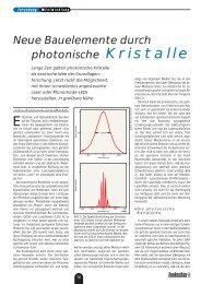
We consider a plane wave S(L, y, z) = Io incident upon a
slab. A schematic view is given in Fig. 1. A spherical
object with radius a is located at ro = (x 0, 0,0). We must
write the potential for a point charge and apply the boundary
condition given by Eq. (2), with S(y, z) = 0. This results
in a summation over mirror images, the outcome
being the diffusion propagator for a slab. The potential
for a dipole can easily be obtained from this result if one
takes the derivative with respect to the position of the
charge. The intensity in the slab can be expressed as
1 1
L I~r = IoL + Jr |ro + 2Lnx|' Jr + r + 2Ln52|
P nE -[(X -
x - x + 2nL
xo + 2nL) 2 + p2 ] 3 / 2
x + x + 2nL
[(x + x + 2nL) 2 + 2]312'
with x being a unit vector along the x axis and p 2 =
y 2 + z 2 .
The first term in Eq. (9) describes the undisturbed intensity,
the second term represents the effect of absorption
analogous to a charge in electrodynamics, and the
I
0.' .
L
.
Den Outer et al.
Fig. 1. Schematic view of a multiple-scattering system with an
embedded spherical object. The scattering system is characterized
by a diffusion constant DI and the object by radius a, diffusion
constant D 2, and absorbing parameter a. A plane wave is
incident at x = L. The intensity is derived at x = 0 and x = L.
(9)

Den Outer et al.
third is the dipole term from scattering. Further details
of the object will be found in higher multipoles for the
intensity outside the object, but their contribution to the
disturbance far from the object will be small. When a

1212 J. Opt. Soc. Am. A/Vol. 10, No. 6/June 1993
Moreover, a careful reinvestigation of the diagrammatic
analysis employed in Ref. 7 reveals that the result indeed
has the behavior of a dipole rather than of a charge.
B. Two-Dimensional Slab
The disturbance on the intensity for a two-dimensional
slab is derived completely analogously to the previous approach.
To obtain the intensity distribution from a point
source in a two-dimensional system, one has to write
down the potential for a line charge and apply the first
boundary condition of Eqs. (2) with S(L, y, z) = 0. Experimentally
a two-dimensional system can be realized if
one makes the system translationally invariant along one
coordinate; i.e., if one uses rods and glass fibers as objects.
The application of the boundary condition of Eqs. (2) on
the potential for a line charge results in a summation over
mirror images, which can be performed exactly. Here it
is convenient to introduce the complex variable ; = x +
iy. The potential for a line dipole can again be found if
one takes the derivative of this result with respect to the
position. The ansatz for the solution of the diffusion
equation [Eq. (1)] with a line charge and a line dipole outside
the object reads as
I = I x + q~e~n sin[(r/2L)( - x)]
q ~ nsin[(ir/2L)( + x)]J
+ pRe{cot[2(; - xo)] + cot[( + ]1
(18)
where x 0 is the position of the scatterer (yo = 0). For absorption
only at the boundary the ansatz is
Iin(0 = A + B(x - xo). (19)
For uniform absorption the ansatz for the intensity inside
the object is
Iin(;) = AIo(Kp) + 2BI(KP)COS .
K
(20)
Here I(r) and I(r) are the modified Bessel functions of
order 0 and 1, p = IPI = (X 2 + y 2 )1" 2 , and is the angle
between p and the x axis.
To obtain the constants q, p, A, and B we approximate
Eq. (18) for ; close to x0 and for a/L small:
Iout( = Io XO + (x - xo)
{ | 7r [(X-XO)2 + y2]1/2 + a2 2L sin(7r/L)xo VL2
2L(x - x) + a
+ PL 2(x - XO) 2
2]1/2 + cot -x0 + O()
Y LL
(21)
We insert Eqs. (19) and (21) into Eqs. (7) and (8), which
accounts for uniform absorption and absorption on the
surface of the object, to obtain
q = io[L + p cot(irxo/L)]
aa + D 2KaI,(Ka)/Io(Ka)
D1 + [aa + D2KaI(Ka)/IO(Ka)]ln(L/a*)
ira 2 Di - D 2[KaIo(Ka) - Il(Ka)]/I1(Ka) - aa
O2L2 D + D 2[KaIo(Ka) - Il(Ka)]/II(Ka)
+ aa
A IO(Ka) D
KaIi(Ka)D 2+ I(aa
B = 21(a) (I1 + P 2L)
with the rescaled radius
sra
a 2 sin(7rfxolL)
(22)
(23)
Although the dipole term depends on a and K separately,
we take K = 0 from now on. This simplification is justified
because the dipole contribution to the intensity disturbance
can be neglected whenever absorption is present.
One may conclude that the intensity disturbance far outside
the object does not depend dramatically on specific
mechanism of absorption. For K = 0, the coefficients reduce
to
rxo D 1 - D 2 - aa ra 2
q IOLL uIDI + D 2 + aa 2L2J
aa
x D1 + aa ln(L/a*)
A Dlq
aa
D - D2 - aa 7ra 2
DI + D 2 + aa 2L 2
B = Io± + Pai-
L
(24)
When aa > Da 2 /L 2 , the charge term dominates and has
strength [ln(L/a*) + D/aa] . We obtain for the transmitted
light
_1 aIr)
T(y) = -- a
Io x _o
I r ir sin(.7rxo/L)
L cosh(,7ry/L) - cos(,7rxo/L)
and for the backscattered light
B (y) -1 - - |
Io ax x-L
2Xp 1 - cosh(7ry/L)cos(7rxo/L)
[cosh(7ry/L) - cos(,7rxo/L)]2J
1 + 7r sin(7rxo/L)
L cosh(ry/L) + cos(irxo/L)
- 1 + cosh(iry/L)cos(irxo/L) 1
[cosh(ry/L) + cos(lrxo/L)]2J
Den Outer et al.
(25)
(26)

Den Outer et al.-
1 .00
0.95
0.90
'E 0.85
C
4 0.80
S
0.75
t 0.70
'0.65
0.60
0.55 -20
1.005
1.004 -
a 1 .003
C al
. 1.002
Z 1.001
'E
1.000
-16 -12 -8 -4 0 4 8 1 2 1 6 20
transversal position (mm)
(a)
0.999
-20 -16 -12 -8 -4 0 4 8 12 1 6 20
transversal position (mm)
(b)
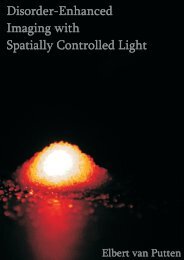
Fig. 2. Calculated diffuse intensities are shown for an object
embedded in a two-dimensional multiple scattering system, as a
function of the transversal distance to the object. The intensity
is plotted relative to the undisturbed intensity (no object present),
according to Eq. (26). (a) Transmission for absorbing rod,
a = 1, a = a, K = 0. Solid curve, xo = 20 1; dotted curve, x0 =
80 1. (b) Transmission for scattering rod, a = ,a = K = 0,
D2 = m. Solid curve, x0 = 20 1; dotted curve, xo = 30 1; dashed
curve, xo = 40 1. In all cases L = 100 1. L is the thickness of the
slab, and 1 is the mean free path.
A few examples are plotted in Fig. 2 for different
tions and absorption coefficients.
C. Point Source
It is often more convenient to use a point source instei
a plane wave, and also the quality of the image can be
proved when the response of the system on a point so
is known. 7 To calculate this response, first one sh
know the intensity distribution in the slab that is dt
the point-source incidence in the absence of an oh
According to Akkermans et al.,1 6 one can make thE
sumption that all the incoming light starts to propa
diffusely at one transport mean free path inside the
Without an object, the intensity distribution inside
slab is given by
G~l, Ren sin[(r/2L)- 1)]
G'lI) - ~n sin[(,r/2L)(; + 1)]J
for a two-dimensional system and by
G(l,
r) =2 1 zi /
[(1 l - x + 2Ln) 2 + y2 + z2 ]" 2
[(I + x + 2Ln) 2 + y 2 + z 2 ]1/2
Vol. 10, No. 6/June 1993/J. Opt. Soc. Am. A 1213
for a three-dimensional system. Since a point source is
used, the ansatz for the solution of the total problem, medium
plus object, will change. One should realize that the
direction of the dipole depends on the local light flux.
The direction of the flux at a particular point is now a
function of position. The new ansatz in two dimensions
reads as
with
R sin[(ir/2L)(; - x0 - iyo)]
= I0 G(l;) + q Reln sin[(ir/2L)(; + x0 + iyo)]J
+ Re cot[ x 0 + iyo)]
+ p*cot[jj§(; + X0 - iyO) (29)
p _js,(xo,yo) + iS 2(Xo,Yo)- (30)
The coefficients s, (x 0, yo) and s 2(xO, yO) follow from a firstorder
Taylor expansion,
sin[(Qn/L)(xo - 1)]
= cosh[(7r/L)yo] - cos[(r/L)(xo - 1)]
sin[(7r/L)(xo + 1)]
cosh[(ir/L)yo] - cos[(ir/L)(xo + 1)]
sinh[( 7/L)yo]
= cosh[(ir/L)yo] - cos[(/L)(xo - 1)]
sinh[(1r/L)xo]
cosh[(r/L)yo] - cos[(rr/L)(xo - 1)] (31)
Also, the intensity inside the object should be adjusted to
the local flux direction:
'in = A + B[s,(xoyo)(x - xo) + s2(xOyo)(y - yo)]-
(32)
Now one can perform a straightforward calculation to
obtain the coefficients q, p, A, and B. They are
q = [IoG(l, o) + fis,(xo,yo)cot(lrxo/L)]D + aaln(L/a*)
A = Diq/aa,
i7a 2 D -D2 - aa
2L! DI + D2 + aa
B I 2D, (33)
2L D, + D 2 + aa
(27) In three dimensions the new ansatz reads as
Iout(r) = IoG(1,r) + qIq(r) + p-| G(1,r)
ar ro
(28) Iin(r) = A + B(r - ro) . - G(l, r),
ar r
d Iq(r),
ar ( (34)
(35)

1214 J. Opt. Soc. Am. A/Vol. 10, No. 6/June 1993
0.35
0.30
0.25
,0.20 /
.10.10/ Z005 . /X ll
0.05
0.00 -
-1 6.0 -12.0 -8.0 -4.0 0.0 4.0 8.0 12.0 1 6.0 20.0
transversal position (mm)
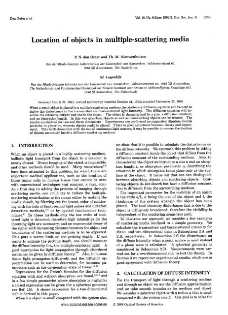
Fig. 3. Calculated transmitted diffuse intensities as a function
of the transversal distance y for a slab containing an absorbing
spherical object at various positions, following Eq. (16). The light
source is pointlike and placed at r= (1,0,0). Slab thickness
L = 50 1, absorbing object radius a = , = , scattering term
neglected. Solid curve, no object; long-dashed curve, x =
45 ,yo = 0; dashed-dotted curve, x = 45 ,yo = 10 1; shortdashed
curve, xo = 5 1, yo = 0; dotted curve x 0 = 5 1, yo = 10 1.
where
nIr [(x - xo + 2Ln) 2 + (y - yo) 2 + (z - Z2]12
1
[(x + x 0 + 2Ln) 2 + (y - yo) 2 + (Z - ZO)2]112
(36)
The coefficients q, p, A, and B follow again from boundary
conditions (7) and (8). This results in
q = -aIOG(, rO) aa'
D + aa
= D - D2- a
a 3 IO 2 D + D 2 + a
A =Dq
aa2
B = + 3D+ D1
2,+ D2 + aa~
q = -a[IoGR(rsrO) - p ro
p = a 3 I 0a- GR(r, r)2
A = _ Dlq
aa2
The disturbance on the intensity depends strongly on
the position of the light source. The disturbance can be
more pronounced than for plane-wave incidence, depending
on the relative distance between the object and the
light source. This is a more convenient situation because
now a displacement of the source can give either a background
measurement (without an object) or a measurement
with an object. A few examples are plotted in Fig. 3.
The transmitted intensity is plotted for various positions
of the object with respect to the point source and the
boundaries of the slab. The strong dependence of the
transmitted intensity on the position of the object is readily
seen from the figure.
D. Spherical Geometry
An expression for the light intensity is derived for a
spherical medium in which an object has been placed.
First we must know the diffusion propagator, or the
Green's function, for a sphere. When absorption is absent
or negligible, a closed expression can easily be obtained
with the help of only one mirror image. 5 We will use this
Green's function to calculate the disturbance. A point
source is used and placed at the positive z axis at one
transport mean-free path underneath the surface of the
sphere' 6 : r, = (O,O,R - ). So the intensity inside the
sphere of radius R, in the absence of an object, is given by
I(r) = IGR(r,r). (38)
The Green's function for a sphere is given by
1
GR (rl,r 2) = I 2
R 1
r2 R2
ri - _X`2
r22
(39)
When an object is placed at r inside the sphere, we can
express the intensity as
Iout(r) = I(r) + qGR(r,ro) - P a GR(rro).
aro
Inside the sphere we use the ansatz
(40)
Iin = A + IoB (r - r). (41)
We use boundary conditions (7) and (8) to derive the
coefficients
R 1 cia
2 (r0 - R2)2J Di + aa[l 2 - 2 aR/(rb - R )]
D- -D2-aa
al. ro 2D,[1 - /2 a3R3 2 /(r0 -
2 3 R ) ] + (D2 + aa)[1 + a 3 R3/(r 2 R
-R2)3]
+qor2- R 22DJ[1 - /2 a R 3 /(ro 2
a R [I R 3
ar ro (ro2 i) 3+(
0 2 -R23
D, + D 2 + aa
- R 2 ) 3 ] + (D 2 + aa)[1 + a3R 3 /(ro 2 - R2)3]
Den Outer et al.
(42)
(43)
(44)
(45)
The coefficients q and p are still to be obtained from
Eqs. (42) and (43). But the above form permits an easy
comparison with the former obtained coefficients. The
transmission through the surface of the sphere can be
found if one takes the normal derivative.

Den Outer et al.
OBJECT
S Le D
Fig. 4. Experimental setup: L, laser, Sp, spatial filter; S,
screen; C, cell with the scattering medium and the object; Le,
lens for imaging the diffuse intensity on D, the one-dimensional
diode array.
1.050
1 .000
0.950
0.900 M
O0.850 -
0.800 c
C
S0.750 .
transversal position (mm)
Fig. 5. Transmitted intensity profiles from a cell containing a
diffusive scattering suspension, for various positions of the embedded
absorbing wire 4 = 350 ,m: a, x0 = 1.00 mm; b,
xO= 2.60 mm, and c, x0 = 4.10 mm. The experimental data are
shown together with the best numerical fits for Eq. (25): a, x0 =
1.41 ± 0.05 mm, D,/oaa = 0.95 ± 0.03; b, x0 = 2.86 + 0.05 mm,
Di/ara = 1.04 + 0.03; c, xo = 4.33 + 0.05 mm, D,/aa = 1.11 ±
0.03. In all cases a = 0.175, bm, p = 0, 1 = 20 ± 3 and cell
thickness L = 10.0 mm.
3. MEASUREMENTS
The experimental setup for a plane-wave transmission
measurement is shown in Fig. 4. A 7-mW continuouswave
He-Ne laser beam (A = 633 nm) is spatially filtered
and expanded to a radius of approximately 20 cm to produce
a flat beam profile. Part of this beam impinges upon
the cell with the object in the highly scattering medium.
The transmitted light, imaged on a one-dimensional diode
array, is read out by a computer. The spatial resolution is
approximately 60 jum. When backscattering experiments
Vol. 10, No. 6/June 1993/J. Opt. Soc. Am. A 1215
are done, the illuminated side of the cell is imaged on the
diode array. Care should be taken for the window ref lection
of the cell. We have used two different cells. The
first has a thickness of 4 mm and 4 mm X 40 mm X
40 mm sized windows, the second has a variable thickness
of 5 or 10 mm and windows with size 20 mm X 60 mm X
60 mm. Complications are introduced by the glass windows,
since light is totally reflected by the window-air
interface when the angle between the surface normal and
the light ray is beyond the critical angle. This reflected
light either enters the sample again or is reflected by it.
As a consequence, every point source at the boundary of
the scattering medium is spread out in a triangular intensity
profile, and a nonnegligible deformation of the intensity
occurs. Transmission experiments on absorbing
objects suffer most from this effect, because the intensity
profile relative to the background is the largest.
This deformation can be reproduced if one convolutes
the calculated profiles with the triangular intensity profile.
The latter should be calculated on the basis of multiple
reflections inside the window. However, this will
extend the fitting procedure by the introduction of more
fit parameters, and therefore the procedure is not
favorable.
We have chosen to reduce the effect of these reflections
on the intensity profile by using a cell with thick windows.
The total internal reflected light is well separated from its
source, and in most cases the light is reflected beside the
sample. (An antireflection coating on the windows would
not have solved this problem because the coating cannot
reduce total internal reflections.)
For plane-wave incident experiments we perform ratio
measurements to correct for the sensitivity of the individual
diodes and to correct for the remaining beam profile.
Depending on the strength of the signal, integration times
vary from 10 s to 3 min. The scattering medium consists
of suspended TiO 2 rutile particles, having an average size
of 220 nm, in glycerine. We calculate the transport meanfree
path from the measured scattering mean-free path by
means of Mie theory.' 0
In Fig. 5 we present transmission measurements for absorbing
rods. We use a 0.35-mm pencil embedded in a
scattering medium with a transport mean-free path of
20 tum. The thickness of the cell is 10.0 mm. The solid
curves are the best numerical fits of Eq. (25) to the measured
profiles. Here the position and the absorbing
Table 1. Fits of the Calculated Line Shape to Experimental Data Obtained from a Transmission
Experiment with an Absorbing Roda
Experimental Fitted Absorption Experimental Fitted Position
Normal Normal Strength Position Relative to Relative to
Position (mm) Position (mm) D/aa First Position (mm) First Position (mm)
0.75 ± 0.05 1.23 ± 0.02 0.95 ± 0.03 0 0
1.40 ± 0.05 1.91 ± 0.02 0.99 ± 0.03 0.65 ± 0.07 0.68 ± 0.03
2.30 ± 0.05 2.78 ± 0.02 1.04 ± 0.03 1.55 ± 0.07 1.55 ± 0.03
3.50 ± 0.05 3.91 ± 0.02 1.10 ± 0.03 2.75 ± 0.07 2.68 ± 0.03
4.95 ± 0.05 5.28 ± 0.02 1.11 ± 0.03 4.20 ± 0.07 4.05 ± 0.03
6.30 ± 0.05 6.67 ± 0.02 0.96 ± 0.03 5.55 ± 0.07 5.44 ± 0.03
7.80 ± 0.05 8.2 ± 0.1 0.8 ± 0.1 7.05 ± 0.07 7.0 ± 0.1
9.30 ± 0.05 9.8 ± 0.1 0.6 ± 0.1 8.55 ± 0.07 8.6 ± 0.1
aIn all cases the scattering contribution is neglected, p = 0; the size of the rod 0 = 350 Am, and the diffusion constant inside the rod D 2

1216 J. Opt. Soc. Am. A/Vol. 10, No. 6/June 1993
.>1 .0
C'
.
X 0.8
C
ffi0.7
2
g 0.6
E 0.5
C
r
u. t 0 1 2 3 4 5 6 7 8
fitted normal position (mm)
9 10
Fig. 6. Minima of the intensity profiles for different positions of
the absorbing wire. The experimental points of Table 1 are plotted.
The solid curve is obtained from Eq. (25) with L = 10.0 mm,
a = 0.175 mm, D,/aa = 1.00, p = 0, and D 2 = 0.
Table 2. Fits of the Calculated Line Shape to
Transmission Experiment Data'
Experimental Transversal Fitted Transversal
Displacement (mm) Displacement (mm)
2.00 ± 0.02 2.05 ± 0.03
4.00 ± 0.02 4.04 ± 0.06
5.00 ± 0.02 5.02 ± 0.07
7.00 ± 0.02 7.03 ± 0.09
9.00 ± 0.02 9.1 0.1
11.00 ± 0.02 11.1 ± 0.2
aExperimental displacements of an absorbing rod parallel to the slab are
compared with those obtained from the corresponding fits. The distance
between the rod and the boundary (x position) is 4.30 ± 0.02 mm, and the
thickness of the cell is 10.0 mm. The scattering contribution is neglected
(p = 0), and the diffusion constant inside the rod is small (D 2

Den Outer et al.
Table 3. Fits of the Calculated Line Shape to Experimental Data Obtained from a Backscatter
Experiment with an Absorbing Roda
Experimental Fitted Absorption Strength
Normal Position (mm) Normal Position (mm) D/iaa
0.28 ± 0.05 0.34 ± 0.02 0.5 ± 0.1
0.78 ± 0.05 0.82 ± 0.02 0.6 ± 0.1
1.38 ± 0.05 1.32 ± 0.02 2.0 ± 0.1
1.68 ± 0.05 1.7 ± 0.1 1.7 ± 0.1
Ax = 50 + 5 Am
Ax = 48 3 Amb
aThe size of the rod 0 = 350 tim, and the thickness of the cell is 4 mm. The scattering contribution is neglected (p = 0). The diffusion constant inside
the rod D2

1218 J. Opt. Soc. Am. A/Vol. 10, No. 6/June 1993
formation on the size and on the absorption strength can
be obtained when the transmitted intensity can be
recorded for various normal positions of the object.
The visibility of an object scales with the ratio aL, a
being the object and L the sample size, because diffuse
intensity is measured.
ACKNOWLEDGMENTS
The authors thank Shechao Feng for initiating the experiment,
Jean-Marc Luck for drawing attention to the application
of diffusion theory, and Meint van Albada and
Johannes de Boer for helpful discussions. This work
is part of the research program of the Stichting voor
Fundamenteel Onderzoek der Materie, which is financially
supported by Nederlandse Organisatie voor Wetenschappelijk
Onderzoek. The work of Nieuwenhuizen has been
made possible by a fellowship of the Royal Netherlands
Academy of Arts and Sciences.
REFERENCES AND NOTES
1. S. R. Arridge, P. van der Zee, M. Cope, and D. T. Delpy,
"Reconstruction methods for infra-red absorption imaging,"
in Time-Resolved Spectroscopy and Imaging of Tissues,
B. Chance and A. Katzir, eds., Proc. Soc. Photo-Opt. Instrum.
Eng. 1431, 204-351 (1991).
2. D. T. Delpy, M. Cope, P. van der Zee, S. Wray, and J. Wyatt,
"Estimation of optical pathlength through tissue from direct
time of flight measurement," Phys. Med. Biol. 33, 1433-1442
(1988).
3. H. Chen, Y. Chen, D. Dilworth, E. Leith, J. Lopez, and
J. Valdmanis, "Two-dimensional imaging through diffusing
media using 150-fs gated electronic holography techniques,"
Opt. Lett. 16, 487-489 (1991).
4. K. M. Yoo, Q. Xing, and R. R. Alfano, "Imaging objects hidden
in highly scattering media using femtosecond second-
Den Outer et al.
harmonic-generation cross-correlation time gating," Opt.
Lett. 16, 1019-1021 (1991).
5. R. W Waynant, presider, session on biomedical imaging, in
Conference on Lasers and Electro-Optics, Vol. 10 of 1991
OSA Technical Digest Series (Optical Society of America,
Washington, D.C., 1991), pp. 101-104.
6. E. N. Leith, C. Chen, H. Chen, Y Chen, J. Lopez, and P. C.
Sun, "Imaging through scattering media using spatial incoherence
techniques," Opt. Lett. 16, 1820-1822 (1991).
7. R. Berkovits and S. Feng, "Theory of speckle-pattern tomography
in multiple-scattering media," Phys. Rev. Lett. 65,
3120-3123 (1990).
8. I. Freund, "Image reconstruction through multiple scattering
media," Opt. Commun. 86, 216-227 (1991).
9. A. Ishimaru, Wave Propagation and Scattering in Random
Media (Academic, New York, 1978), Vols. I and II.
10. H. C. van de Hulst, Multiple Light Scattering (Academic,
New York, 1980), Vols. I and II.
11. J. Fishkin, E. Gratton, M. J. van de Ven, and W W Mantulin,
"Diffusion of intensity modulated near-infrared light in turbid
media," in Time-Resolved Spectroscopy and Imaging of
Tissues, B. Chance and A. Katzir, eds., Proc. Soc. Photo-Opt.
Instrum. Eng. 1431, 122-135 (1991).
12. S. R. Arridge, M. Cope, P. van der Zee, P. J. Hilson, and D. T.
Delpy, "Visualization of the oxygenation state of brain and
muscle in newborn infants by near infra-red transillumination,"
in Information Processing in Medical Imaging, S. L.
Bacharach, ed. (Nijhoff, Dordrecht, 1985), pp. 155-177.
13. E. M. Sevick, B. Chance, J. Leigh, S. Nioka, and M. Maris
"Quantitation of time- and frequency-resolved optical spectra
for the determination of tissue oxygenation," Ann. Biochem.
Exp. Med. 195, 330-351 (1991).
14. M. B. van der Mark, M. P. van Albada, and A. Lagendijk,
"Light scattering in strongly media: multiple scattering and
weak localization," Phys. Rev. B 37, 3575-3592 (1988).
15. See, for instance, J. D. Jackson, Classical Electrodynamics
(Wiley, New York, 1975).
16. E. Akkermans, P. E. Wolf, and R. Maynard, "Coherent backscattering
of light by disordered media: analysis of the peak
line shape," Phys. Rev. Lett. 56, 1471-1474 (1986).
17. See, for instance, J. W Goodman, Statistical Optics (Wiley,
New York, 1985).