Soil Classification (AASHTO and USCS)
Soil Classification (AASHTO and USCS)
Soil Classification (AASHTO and USCS)

Create successful ePaper yourself
Turn your PDF publications into a flip-book with our unique Google optimized e-Paper software.
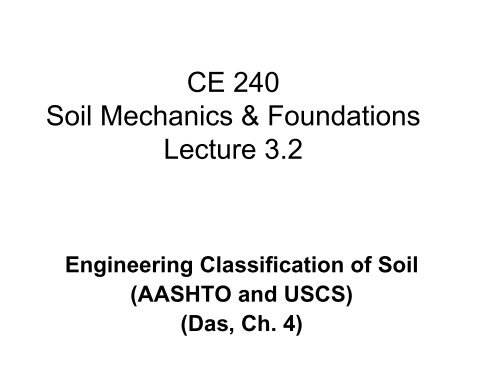
CE 240<br />
<strong>Soil</strong> Mechanics & Foundations<br />
Lecture 3.2<br />
Engineering <strong>Classification</strong> of <strong>Soil</strong><br />
(<strong>AASHTO</strong> <strong>and</strong> <strong>USCS</strong>)<br />
(Das, Ch. 4)
Outline of this Lecture<br />
1. Particle distribution <strong>and</strong> Atterberg Limits<br />
2. <strong>Soil</strong> classification systems based on<br />
particle distribution <strong>and</strong> Atterberg Limits<br />
3. American Association of State Highway <strong>and</strong><br />
Transportation Officials System (<strong>AASHTO</strong>)<br />
4. The Unified <strong>Soil</strong> <strong>Classification</strong> System<br />
(<strong>USCS</strong>)
Objective<br />
Classifying soils into groups with similar<br />
behavior, in terms of simple indices, can<br />
provide geotechnical engineers a general<br />
guidance about engineering properties of the<br />
soils through the accumulated experience.<br />
Simple indices<br />
GSD, LL, PI<br />
Communicate<br />
between<br />
engineers<br />
<strong>Classification</strong><br />
system<br />
(Language)<br />
Use the<br />
accumulated<br />
experience<br />
Estimate<br />
engineering<br />
properties<br />
Achieve<br />
engineering<br />
purposes
<strong>Classification</strong> Systems<br />
• Two commonly used systems for soil<br />
engineers based on particle distribution<br />
<strong>and</strong> Atterberg limits:<br />
• American Association of State Highway<br />
<strong>and</strong> Transportation Officials (<strong>AASHTO</strong>)<br />
System (for state/county highway dept.)<br />
• Unified <strong>Soil</strong> <strong>Classification</strong> System (<strong>USCS</strong>)<br />
(preferred by geotechnical engineers).
<strong>Soil</strong> particles<br />
The description of the grain size distribution of soil<br />
particles according to their texture (particle size,<br />
shape, <strong>and</strong> gradation).<br />
Major textural classes include, very roughly:<br />
gravel (>2 mm);<br />
s<strong>and</strong> (0.1 – 2 mm);<br />
silt (0.01 – 0.1 mm);<br />
clay (< 0.01 mm).<br />
Furthermore, gravel <strong>and</strong> s<strong>and</strong> can be roughly<br />
classified as coarse textured soils, wile silt <strong>and</strong> clay<br />
can be classified as fine textures soils.
Cobbles or Boulders<br />
Grain Size Distribution Curves<br />
GRAVEL SAND FINES
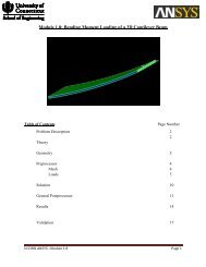
Atterberg limits<br />
Atterberg limits are the limits of water content used to<br />
define soil behavior. The consistency of soils according<br />
to Atterberg limits gives the following diagram.
American Association of State<br />
Highway <strong>and</strong> Transportation<br />
Officials system (<strong>AASHTO</strong>)<br />
Origin of <strong>AASHTO</strong>: (For road construction)<br />
This system was originally developed by<br />
Hogentogler <strong>and</strong> Terzaghi in 1929 as the Public<br />
Roads <strong>Classification</strong> System. Afterwards, there are<br />
several revisions. The present <strong>AASHTO</strong> (1978)<br />
system is primarily based on the version in 1945.<br />
(Holtz <strong>and</strong> Kovacs, 1981)
Definition of Grain Size<br />
No specific grain<br />
size-use<br />
Atterberg limits<br />
Boulders Silt-Clay<br />
Gravel S<strong>and</strong><br />
75 mm<br />
No.4<br />
4.75 mm<br />
Coarse Fine<br />
No.40<br />
0.425 mm<br />
No.200<br />
0.075<br />
mm
<strong>Classification</strong><br />
(Proceeding from left to right against the columns)<br />
Das, Table 4.1, 2006
Note:<br />
<strong>Classification</strong> (Cont.)<br />
The first group from the left to fit the test data is the<br />
correct <strong>AASHTO</strong> classification.<br />
Das, Table 4.1, 2006
Group Index GI<br />
200<br />
200<br />
[ ]<br />
GI = ( F − 35) 0.2 + 0.005( LL −40)<br />
+ 0.01( F −15)( PI −10)<br />
(4.1)<br />
For Group A-2-6 <strong>and</strong> A-2-7<br />
200<br />
The first term is determined by the LL<br />
The second term is determined by the PI<br />
GI = 0.01( F −15)( PI −10) (4.2) use the second term only<br />
F200: percentage passing through the No.200 sieve<br />
In general, the rating for a pavement subgrade is<br />
inversely proportional to the group index, GI.
Some Explanations of Group Index GI<br />
1, if Eq. 4.1 gives a negative value then GI=0;<br />
2, round up the value calculated by Eq. 4.1 to<br />
an integer;<br />
3, there is no upper limit for GI;<br />
4, the GIs for soil groups A-1-a, A-1-b, A-2-4,<br />
A-2-5, <strong>and</strong> A-3 are always zero (0).
(PI)<br />
(LL)<br />
Das, Figure 4.1
General Guidance<br />
– 8 major groups: A1~ A7 (with several subgroups) <strong>and</strong><br />
organic soils A8<br />
– The required tests are sieve analysis <strong>and</strong> Atterberg<br />
limits.<br />
– The group index, an empirical formula, is used to<br />
further evaluate soils within a group (subgroups).<br />
A1 ~ A3<br />
Granular Materials<br />
≤ 35% pass No. 200 sieve<br />
Using LL <strong>and</strong> PI separates silty<br />
materials from clayey materials (only<br />
for A2 group)<br />
A4 ~ A7<br />
Silt-clay Materials<br />
≥ 36% pass No. 200 sieve<br />
Using LL <strong>and</strong> PI separates silty<br />
materials from clayey materials<br />
– The original purpose of this classification system is<br />
used for road construction (subgrade rating).
Example 4.1, <strong>Soil</strong> B<br />
Passing No.200 86%<br />
LL=70, PI=32<br />
LL-30=40 > PI=32<br />
GI<br />
= ( F<br />
200<br />
+ 0.<br />
01(<br />
F<br />
=<br />
33.<br />
47<br />
− 35)<br />
200<br />
≅<br />
33<br />
[ 0.<br />
2 + 0.<br />
005(<br />
LL − 40)<br />
]<br />
−15)(<br />
PI −10)<br />
Round off<br />
A-7-5(33)
This is the example<br />
of Das, Example 4.1<br />
for the <strong>AASHTO</strong><br />
system classification
<strong>USCS</strong> <strong>Classification</strong> System<br />
• Originally developed for the United<br />
States Army Corps of Engineers<br />
(USACE)<br />
• The method is st<strong>and</strong>ardized in ASTM D<br />
2487 as “Unified <strong>Soil</strong> <strong>Classification</strong><br />
System (<strong>USCS</strong>)”<br />
• <strong>USCS</strong> is the most common soil<br />
classification system among<br />
geotechnical engineers
Unified <strong>Soil</strong> <strong>Classification</strong> System<br />
Origin of <strong>USCS</strong>:<br />
(<strong>USCS</strong>)<br />
This system was first developed by Professor A.<br />
Casagr<strong>and</strong>e (1948) for the purpose of airfield<br />
construction during World War II. Afterwards, it was<br />
modified by Professor Casagr<strong>and</strong>e, the U.S. Bureau of<br />
Reclamation, <strong>and</strong> the U.S. Army Corps of Engineers to<br />
enable the system to be applicable to dams,<br />
foundations, <strong>and</strong> other construction.<br />
Four major divisions:<br />
(1) Coarse-grained<br />
(2) Fine-grained<br />
(3) Organic soils<br />
(4) Peat
Boulders<br />
Definition of Grain Size<br />
Cobbles<br />
300 mm<br />
75 mm<br />
Gravel S<strong>and</strong><br />
Coarse Fine Coarse Medium Fine<br />
No.4<br />
4.75 mm<br />
19 mm No.10 No.40<br />
2.0 mm<br />
No specific grain sizeuse<br />
Atterberg limits<br />
0.425 mm<br />
No.200<br />
0.075<br />
mm<br />
Silt <strong>and</strong><br />
Clay
(Das, Table 4.2)
• <strong>Soil</strong> symbols:<br />
• G: Gravel<br />
• S: S<strong>and</strong><br />
• M: Silt<br />
• C: Clay<br />
• O: Organic<br />
• Pt: Peat<br />
Example: SW, Well-graded s<strong>and</strong><br />
SC, Clayey s<strong>and</strong><br />
SM, Silty s<strong>and</strong>,<br />
MH, Elastic silt<br />
The Symbols<br />
• Liquid limit<br />
symbols:<br />
• H: High LL (LL>50)<br />
• L: Low LL (LL
<strong>USCS</strong> System (cont.)<br />
• A typical <strong>USCS</strong> classification would be:<br />
Group<br />
Symbol<br />
-<br />
SM Silty s<strong>and</strong> with gravel<br />
Group<br />
Name
<strong>Classification</strong> of <strong>Soil</strong>s<br />
• From sieve analysis <strong>and</strong> the grain-size<br />
distribution curve determine the percent<br />
passing as the following:<br />
– > 3 inch – Cobble or Boulders<br />
– 3 inch - # 4 (76.2 – 4.75 mm) : Gravel<br />
– # 4 - # 200 (4.75 - 0.075 mm) : S<strong>and</strong><br />
– < # 200: Fines<br />
• First, Find % passing # 200<br />
• If 5% or more of the soil passes the # 200<br />
sieve, then conduct Atterberg Limits (LL &<br />
PL)
<strong>Classification</strong> of <strong>Soil</strong>s<br />
• If the soil is fine-grained (≥ 50% passes<br />
#200) follow the guidelines for fine-grained<br />
soils<br />
• If the soil is coarse-grained (
50%<br />
General Guidance<br />
Coarse-grained soils:<br />
Gravel S<strong>and</strong><br />
•Grain size distribution<br />
•C u<br />
•C c<br />
NO. 4<br />
4.75 mm<br />
50 %<br />
NO.200<br />
0.075 mm<br />
Required tests: Sieve analysis<br />
Fine-grained soils:<br />
Silt Clay<br />
Atterberg limit<br />
•PL, LL<br />
•Plasticity chart<br />
LL>50<br />
LL
Coarse-grained <strong>Soil</strong>s
Fine-grained <strong>Soil</strong>s
Gravel<br />
98-62 = 36%<br />
S<strong>and</strong><br />
62-8 = 54%<br />
Fines = 8%<br />
Example – <strong>Soil</strong> A<br />
gravel s<strong>and</strong> fines<br />
<strong>Soil</strong> A: D 60 = 4.2 mm , D 30 = 0.6 mm, D 10 = 0.09 mm<br />
Cu = 46.67<br />
Cc = 0.95
Grave = 36%<br />
S<strong>and</strong> = 54%<br />
Fines = 8%<br />
Cu = 46.7<br />
Cc = 0.95<br />
LL = 42<br />
PL = 31<br />
PI = 42-31 = 11<br />
GO TO Plasticity<br />
Chart<br />
Example – <strong>Soil</strong> A (Cont.)
Example – <strong>Soil</strong> A (Cont.)<br />
• <strong>Soil</strong> A is then classified as<br />
SP-SM – Poorly-grades s<strong>and</strong> with silt <strong>and</strong><br />
gravel
LL = 42<br />
PL = 31<br />
PI = 42-31 = 11<br />
Example – <strong>Soil</strong> A (Cont.)<br />
ML
PI<br />
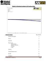
The Plasticity Chart<br />
L<br />
H<br />
LL<br />
(Holtz <strong>and</strong> Kovacs, 1981)<br />
• The A-line generally<br />
separates the more<br />
claylike materials<br />
from silty materials,<br />
<strong>and</strong> the organics<br />
from the inorganics.<br />
• The U-line indicates<br />
the upper bound for<br />
general soils.<br />
Note: If the measured<br />
limits of soils are on<br />
the left of U-line,<br />
they should be<br />
rechecked.
Procedures for <strong>Classification</strong><br />
Coarse-grained<br />
material<br />
Grain size<br />
distribution<br />
Fine-grained<br />
material<br />
LL, PI<br />
Highly<br />
(Santamarina et al., 2001)
Example<br />
Passing No.200 sieve 30 %<br />
Passing No.4 sieve 70 %<br />
LL= 33<br />
PI= 12<br />
PI= 0.73(LL-20), A-line<br />
PI=0.73(33-20)=9.49<br />
SC<br />
(≥15% gravel)<br />
Clayey s<strong>and</strong> with<br />
gravel<br />
Passing No.200 sieve 30 %<br />
Passing No.4 sieve 70 %<br />
Highly<br />
LL= 33<br />
PI= 12<br />
(Santamarina et al., 2001)
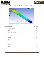
Organic <strong>Soil</strong>s<br />
Highly organic soils- Peat (Group symbol PT)<br />
− A sample composed primarily of vegetable tissue in<br />
various stages of decomposition <strong>and</strong> has a fibrous to<br />
amorphous texture, a dark-brown to black color, <strong>and</strong> an<br />
organic odor should be designated as a highly organic<br />
soil <strong>and</strong> shall be classified as peat, PT.<br />
Organic clay or silt( group symbol OL or OH):<br />
− “The soil’s liquid limit (LL) after oven drying is less than<br />
75 % of its liquid limit before oven drying.” If the above<br />
statement is true, then the first symbol is O.<br />
− The second symbol is obtained by locating the values<br />
of PI <strong>and</strong> LL (not oven dried) in the plasticity chart.
This is the Figure 4.7 of Das’ textbook, the scanning<br />
electron micrographs (SEM) for 4 peat samples.
Borderline Cases (Dual Symbols)<br />
For the following three conditions, a dual<br />
symbol should be used.<br />
–Coarse-grained soils with 5% - 12% fines.<br />
−About 7 % fines can change the hydraulic<br />
conductivity of the coarse-grained media by<br />
orders of magnitude.<br />
−The first symbol indicates whether the coarse<br />
fraction is well or poorly graded. The second<br />
symbol describe the contained fines. For example:<br />
SP-SM, poorly graded s<strong>and</strong> with silt.
Borderline Cases (Dual Symbols, cont.)<br />
–Fine-grained soils with limits within the<br />
shaded zone. (PI between 4 <strong>and</strong> 7 <strong>and</strong> LL<br />
between about 12 <strong>and</strong> 25).<br />
−It is hard to distinguish between the silty <strong>and</strong> more<br />
claylike materials.<br />
−CL-ML: Silty clay, SC-SM: Silty, clayed s<strong>and</strong>.<br />
–<strong>Soil</strong> contain similar fines <strong>and</strong> coarse-grained<br />
fractions.<br />
− possible dual symbols GM-ML
Borderline Cases (Summary)<br />
(Holtz <strong>and</strong> Kovacs, 1981)
Reading Assignment:<br />
Das, Ch. 4<br />
Homework:<br />
Problem 4.3